UNIVERSITÉ DE SHERBROOKE
Faculté de génie
Département de génie électrique et de génie informatique
Cartographie, localisation et planification
simultanées ‘en ligne’, à long terme et à
grande échelle pour robot mobile
Thèse de doctorat
Spécialité : génie électrique
Mathieu LABBÉ
Sherbrooke (Québec) Canada
MEMBRES DU JURY
François MICHAUD
DirecteurPhilippe GIGUÈRE
ÉvaluateurFrédéric MAILHOT
ÉvaluateurFrançois POMERLEAU
ÉvaluateurRÉSUMÉ
Pour être en mesure de naviguer dans des endroits inconnus et non structurés, un robot doit pouvoir cartographier l’environnement afin de s’y localiser. Ce problème est connu sous le nom de cartographie et localisation simultanées (ou SLAM pour Simultaneous Localization and Mapping). Une fois la carte de l’environnement créée, des tâches requérant un déplacement d’un endroit connu à un autre peuvent ainsi être planifiées. La charge de calcul du SLAM est dépendante de la grandeur de la carte. Un robot a une puissance de calcul embarquée limitée pour arriver à traiter l’information ‘en ligne’, c’est-à-dire à bord du robot avec un temps de traitement des données moins long que le temps d’acquisition des données ou le temps maximal permis de mise à jour de la carte. La navigation du robot tout en faisant le SLAM est donc limitée par la taille de l’environnement à cartographier. Pour résoudre cette problématique, l’objectif est de développer un algorithme de SPLAM (Simultaneous Planning Localization and Mapping) permettant la navigation peu importe la taille de l’environment. Pour gérer efficacement la charge de calcul de cet algorithme, la mémoire du robot est divisée en une mémoire de travail et une mémoire à long terme. Lorsque la contrainte de traitement ‘en ligne’ est atteinte, les endroits vus les moins souvent et qui ne sont pas utiles pour la navigation sont transférées de la mémoire de travail à la mémoire à long terme. Les endroits transférés dans la mémoire à long terme ne sont plus utilisés pour la navigation. Cependant, ces endroits transférés peuvent être récupérées de la mémoire à long terme à la mémoire de travail lorsque le le robot s’approche d’un endroit voisin encore dans la mémoire de travail. Le robot peut ainsi se rappeler incrémentalement d’une partie de l’environment a priori oubliée afin de pouvoir s’y localiser pour le suivi de trajectoire.
L’algorithme, nommé RTAB-Map, a été testé sur le robot AZIMUT-3 dans une première expérience de cartographie sur cinq sessions indépendantes, afin d’évaluer la capacité du système à fusionner plusieurs cartes ‘en ligne’. La seconde expérience, avec le même ro-bot utilisé lors de onze sessions totalisant 8 heures de déplacement, a permis d’évaluer la capacité du robot de naviguer de façon autonome tout en faisant du SLAM et plani-fier des trajectoires continuellement sur une longue période en respectant la contrainte de traitement ‘en ligne’ . Enfin, RTAB-Map est comparé à d’autres systèmes de SLAM sur quatre ensembles de données populaires pour des applications de voiture autonome (KITTI), balayage à la main avec une caméra RGB-D (TUM RGB-D), de drone (EuRoC) et de navigation intérieur avec un robot PR2 (MIT Stata Center).
Les résultats montrent que RTAB-Map peut être utilisé sur de longue période de temps en navigation autonome tout en respectant la contrainte de traitement ‘en ligne’ et avec une qualité de carte comparable aux approches de l’état de l’art en SLAM visuel et avec télémètre laser. ll en résulte d’un logiciel libre déployé dans une multitude d’applications allant des robots mobiles intérieurs peu coûteux aux voitures autonomes, en passant par les drones et la modélisation 3D de l’intérieur d’une maison.
REMERCIEMENTS
Tout d’abord, mes recherches furent possibles grâce au support financier du Conseil de recherche en sciences et génie du Canada, la Fondation canadienne pour l’innovation, le programme des Chaires de recherche du Canada et le Fonds de recherche du Québec – Nature et technologies. Je voudrais également remercier la Faculté de génie pour l’oc-troie de la Médaille Léonard deVinci en 2016, ainsi qu’à l’équipe Maxed-Out, un groupe d’utilisateurs de l’environnement de programmation ROS de Silicon Valley, d’avoir choisi RTAB-Map pour gagner la compétition internationale de Kinect à la conférence IEEE International Conference on Intelligent Robots and Systems – IROS en 2014.
De plus, je veux remercier mon directeur de doctorat François Michaud pour sa grande confiance, son soutien, son enthousiaste ainsi que son intérêt pour mon projet. Finalement, je tiens à remercier toute l’équipe du laboratoire IntRoLab pour leur soutien technique et moral tout au long de mes travaux, en particulier les deux autres François, Dominic, Vincent, David, Francis, Michaël, Joël, Ronan, Aurélien, Guillaume et Antoine.
TABLE DES MATIÈRES
1 INTRODUCTION 1
2 Loop Closure Detection for Multi-Session SLAM 5
2.1 Introduction . . . 7
2.2 Online Multi-Session Graph-Based SLAM . . . 9
2.2.1 Loop Closure Detection . . . 9
2.2.2 Graph Optimization . . . 10
2.2.3 Memory Management for Online Multi-Session Mapping . . . 10
2.3 Results . . . 12
2.4 Discussion . . . 18
2.5 Conclusion . . . 21
3 Graph-Based SPLAM with Memory Management 23 3.1 Introduction . . . 25
3.2 Related Work . . . 27
3.3 Memory Management for SPLAM . . . 28
3.3.1 Short-Term Memory Module . . . 32
3.3.2 Appearance-based Loop Closure Detection Module . . . 33
3.3.3 Proximity Detection Module . . . 34
3.3.4 Graph Optimization Module . . . 36
3.3.5 Path Planning Modules . . . 36
3.3.6 Patrol Module . . . 41 3.4 Results . . . 42 3.4.1 Influences of MM on SPLAM . . . 44 3.4.2 TPP-MPP Interactions . . . 46 3.4.3 Influences of LTM on TPP . . . 47 3.5 Discussion . . . 52 3.6 Conclusion . . . 55
4 RTAB-Map as an Open-Source SLAM Library 57 4.1 Introduction . . . 59
4.2 Popular SLAM Approaches Available on ROS . . . 62
4.3 RTAB-Map Description . . . 67
4.3.1 Odometry Node . . . 69
4.3.2 Synchronization . . . 75
4.3.3 STM . . . 76
4.3.4 Loop Closure and Proximity Detection . . . 79
4.3.5 Graph Optimization . . . 80
4.3.6 Global Map Assembling . . . 81
4.4 Evaluating Trajectory Performance of RTAB-Map . . . 82
4.4.1 KITTI . . . 84 ix
4.4.2 TUM . . . 87 4.4.3 EuRoC . . . 89 4.4.4 MIT Stata Center . . . 92 4.5 Evaluating Computation Performance between Visual and Lidar SLAM
Configurations with RTAB-Map . . . 98 4.5.1 Examining the Use of RTAB-Map’s Memory Management Mechanism103 4.6 Discussion . . . 105 4.7 Conclusion . . . 109
5 CONCLUSION 111
LISTE DES FIGURES
2.1 Memory management model. . . 11
2.2 Illustration of a local map created from multi-session mapping. . . 12
2.3 AZIMUT-3 robot equipped with a URG-04XL laser range finder and a Kinect sensor. . . 13
2.4 Resulting local maps without (left) and with (right) graph optimizations. . 14
2.5 Results for Map 4 and Map 5. . . 15
2.6 Processing time in relation to the number of nodes processed over time. . . 16
2.7 Top view of the map without optimization after five mapping sessions. . . 16
2.8 Loop closures between the mapping sessions. . . 17
2.9 Five online mapping sessions merged together automatically. . . 17
2.10 Graphs optimized. . . 19
2.11 Global maps . . . 19
2.12 Processing time for each node added to graph. . . 20
3.1 The AZIMUT-3 robot equipped with a URG-04LX laser range finder and a Xtion PRO LIVE sensor. . . 29
3.2 Memory management and control architecture of SPLAM-MM. . . 29
3.3 Illustration of the local map and the global map in multi-session mapping. 32 3.4 Illustration of the role of the Proximity Detection module. . . 35
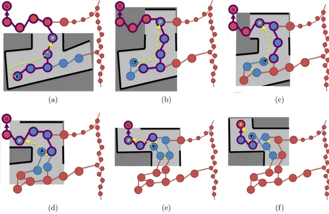
3.5 Illustration of how proximity detection works. . . 37
3.6 Example of obstacle detection using the laser rangefinder and the RGB-D camera. . . 39
3.7 Interaction between TPP and MPP for path planning. . . 41
3.8 Waypoints WP1 to WP4 identified on the global map. The purple path is the first path planned by TPP from the WP4 to WP1. . . 43
3.9 Global maps, optimized and not optimized, after reaching WP1. . . 44
3.10 Events that occurred during the trials. . . 45
3.11 Example of the effect of memory management. . . 45
3.12 Comparison of the corresponding images between the waypoint and at the last pose reached. . . 47
3.13 Memory size and total processing time over the 11 mapping sessions. . . . 48
3.14 Example of poses sent by TPP to MPP. . . 49
3.15 Example where MPP plans a slightly different path than the one provided by TPP. . . 50
3.16 Three examples illustrating how the graph reduction algorithm works. . . . 51
3.17 Comparison between the global maps. . . 53
3.18 Comparison of TPP planning time and LTM size. . . 54
3.19 Comparison of hard drive usage. . . 54
4.1 Block diagram of rtabmap ROS node. . . 68
4.2 Block diagram of rgbd_odometry and stereo_odometry ROS nodes. . . 70 xi
4.3 Block diagram of icp_odometry ROS node. . . 73
4.4 Visual SLAM with a RGB-D camera like the Kinect for Xbox 360. . . 77
4.5 Visual SLAM with a stereo camera like the BumbleBee2. . . 77
4.6 Synchronization example of a RGB-D camera with laser scan and odometry. 78 4.7 STM’s local occupancy grid creation. . . 79
4.8 Global map assembling. . . 82
4.9 Trajectories using RTAB-Map for three KITTI sequences. . . 85
4.10 Trajectories using RTAB-Map for three TUM sequences. . . 88
4.11 Trajectories using RTAB-Map for three EuRoC sequences. . . 91
4.12 Trajectories using RTAB-Map for Stata Center sequences. . . 94
4.13 Comparison of RTAB-Map with other lidar-based SLAM approaches . . . . 97
4.14 Local occupancy grid examples. . . 100
4.15 3D local occupancy grid map with ray tracing examples . . . 101
4.16 2D occupancy grid map examples. . . 102
4.17 OctoMap using RGB-D camera. . . 103
4.18 Processing time required for each module inside rtabmap. . . 105
LISTE DES TABLEAUX
3.1 Parameters used for the trials . . . 43
4.1 Popular ROS-compatible lidar and visual SLAM approaches . . . 66
4.2 RTAB-Map (version 0.16.3) Default Parameters . . . 83
4.3 ATE (m) results for the KITTI sequences . . . 86
4.4 Average translational error (%) results for the KITTI sequences . . . 87
4.5 Current state of KITTI’s odometry leaderboard . . . 88
4.6 ATE (cm) results for the TUM sequences . . . 90
4.7 ATE (cm) results for the EuRoC sequences . . . 90
4.8 Online results for the MIT Stata Center sequences . . . 95
4.9 ATE (m) results of RTAB-Map on 2012-01-25 sequences. . . 99
4.10 Occupancy grid performance . . . 99
CHAPITRE 1
INTRODUCTION
La cartographie et localisation simultanée (SLAM) [Stachniss et coll., 2016] est une ap-proche utilisée en robotique mobile lorsqu’un système de localisation externe comme le GPS n’est pas accessible pour estimer la position précise du robot dans l’environnement. Avec le SLAM, la position du robot est estimée à partir de ses capteurs en relation avec une carte de l’environment construite en même temps. Puisque les capteurs du robot ne sont pas parfaits, des erreurs dans la carte sont introduites, influençant du même coup la précision de la localisation. Pour corriger ces erreurs, le robot doit être en mesure de reconnaître lorsqu’il revient dans un endroit déjà visité : il détecte alors ce qui est qualifié être une fermeture de boucle. Une fois la fermeture de boucle détectée, un algorithme d’optimisation peut être utilisé pour propager l’erreur accumulée dans toute la carte afin de la corriger. La carte générée et la position connue dans celle-ci permettent ensuite de planifier des trajectoires sans collision lors de la navigation.
Pour pourvoir planifier de nouvelles trajectoires pendant que le robot navigue, l’algorithme de SLAM doit respecter la contrainte de traitement ‘en ligne’, c’est -à-dire que le temps de traitement des données doit être moins long que le temps d’acquisition des données ou du temps maximal permis de mise à jour de la carte. Par exemple, si le temps de traitement maximal est fixé à 1 seconde, l’algorithme doit être en mesure de toujours fournir une carte à jour à une fréquence d’au minimum 1 Hz. Lorsqu’un robot fait continuellement du SLAM, la carte construite sera de plus en plus grande si l’environnement n’est pas borné. Ou encore si l’environment est dynamique, il se peut que l’algorithme de SLAM duplique certains endroits [Glover et coll., 2010] ou ait besoin de garder en mémoire plusieurs versions du même endroit pour maximiser la capacité de se localiser par la suite [Churchill et Newman, 2013]. Par exemple, si l’intensité de la lumière change au cours de la journée et que l’algorithme de localisation est basée sur les images, il se peut que garder plusieurs versions du même endroit en mémoire soit bénéfique pour être en mesure de se localiser à la fois le jour et la nuit.
La quantité de mémoire requise par le SLAM peut donc croître indéfiniment. Plus la carte est grande, plus de temps de traitement requis est long pour détecter les fermetures de boucles et pour corriger la carte. Il est donc important d’avoir un mécanisme de gestion de mémoire pour éviter d’avoir à traiter toutes les données à chaque mise à jour de la carte.
Une façon naïve de gestion de mémoire peut être d’éliminer les données les plus vieilles en premier. Le problème avec cette approche est que le robot ne pourra jamais par la suite se re-localiser ou planifier des trajectoires dans cette partie de l’environment. Une gestion de mémoire plus intelligente doit donc être faite pour oublier temporairement des endroits non essentielles à navigation courante afin de limiter le temps de mise à jour de la carte tout en pouvant se rappeler d’anciens endroits lorsque le robot retourne vers ceux-ci. La question de recherche résultante est la suivante : comment intégrer une gestion de mémoire intelligente à un algorithme de SLAM qui permet de respecter la contrainte de traitement ‘en ligne’ à long terme, tout en gardant assez d’information afin d’être en mesure de se localiser globalement et de naviguer dans tous les endroits connus ?
L’approche de gestion de la mémoire présentée dans cette thèse a pour but de réaliser un algorithme de SLAM satisfaisant la contrainte de traitement ‘en ligne’ pour un fonc-tionnement ‘en ligne’ à grande échelle et à long terme. Le temps de traitement, c.-à-d. le temps requis pour traiter une image acquise, est le critère utilisé pour limiter le nombre d’endroits conservés dans la mémoire de travail du robot. Pour identifier les endroits à conserver dans la mémoire de travail, la solution présentée consiste à conserver les en-droits les plus récents et les plus fréquemment observés dans la mémoire de travail, et à transférer les autres dans la mémoire à long terme. Lorsqu’une correspondance est trouvée entre l’endroit actuel et un autre emmagasiné dans la mémoire de travail, les endroits voisins mémorisés dans la mémoire à long terme peuvent être retransférés en mémoire de travail afin de permettre la localisation dans des endroits précédemment “oubliés”. Cette idée est inspirée d’observations faites en psychologie [Baddeley, 1997; Shiffrin, 2003] selon lesquelles les personnes se souviennent davantage des endroits où elles ont passé la plus grande partie de leur temps, comparativement à ceux dont elles ont vus moins souvent. En suivant cette heuristique, le compromis entre le temps et l’espace de recherche est donc fonction de l’environnement et des expériences du robot.
Une première version de cet algorithme de gestion de mémoire a été présentée dans [Labbé et Michaud, 2013] pour le problème spécifique de détection de fermeture de boucle à long terme et à grande échelle. L’approche de détection de fermeture de boucle est basée sur un filtrage bayésien pour estimer les hypothèses de fermeture de boucle. La vraisemblance entre le nouvel et les anciens endroits est calculée par l’approche de sac-de-mots (ou BOW pour bag-of-words). Des repères visuels sont extraits des images et ils sont ensuite quantifiés dans un dictionnaire incrémental de mots visuels. Chaque mot visuel dans le dictionnaire garde une liste des images dans lesquelles il se retrouve. Cet index inversé permet ensuite de comparer très rapidement une image avec une grande banque d’images selon un principe
3 de vote. Pour chaque mot visuel extrait dans l’image courante, les images dans la carte contenant le même mot vont recevoir un vote. L’image avec le plus de votes est la plus similaire à l’image actuelle. Le filtre bayésien estime aussi la probabilité que la nouvelle image provienne d’un nouvel endroit. Si la probabilité de fermeture de boucle d’un endroit connu est au-dessus un seuil prédéfini, une fermeture de boucle est alors détectée, sinon l’image est considérée provenir d’un nouvel endroit. La gestion de mémoire était utilisée pour limiter le temps de mise à jour du filtre bayésien et du dictionnaire de mots visuels afin d’être en mesure de détecter les fermetures de boucle toujours ‘en ligne’. L’approche avait été testée seulement sur des ensembles de données d’images (réelles et synthétiques), il restait à étendre et expérimenter les principes sous-jacents à cet algorithme sur un vrai robot faisant du SLAM et de la navigation ‘en ligne’. Dans cette thèse, ceux-ci sont in-tégrés à un système complet de SLAM et rigoureusement testé sur des robots. De plus, de nouveaux critères de gestion de mémoire ont été ajoutés pour que la navigation auto-nome dans des endroits a priori oubliés soit possible tout en respectant la contrainte de traitement ‘en ligne’.
Le chapitre 2 montre, dans un premier temps, comment la gestion de mémoire peut être intégrée à un algorithme de SLAM sur un robot réel, et ce, dans un contexte multi-sessions, c’est-à-dire combinant plusieurs sessions de SLAM à partir de points de départ différents mais dont les endroits visités se recoupent afin de relier les cartes résultantes de ces sessions. Le chapitre 3 présente ensuite l’algorithme de cartographie, localisation et planification simultanées ‘en ligne’, à long terme et à grande échelle pour robot mobile, soit la contribution centrale de cette thèse. Le chapitre 4 termine en décrivant la librairie de SLAM résultante de la thèse, appelée RTAB-Map, distribuée comme logiciel libre et utilisée par des centaines de développeurs en robotique mobile. En plus de situer RTAB-Map par rapport à l’état de l’art en SLAM et d’évaluer les performances selon le coût et la sorte de capteurs utilisés, une comparaison exhaustive et juste entre les paradigmes de SLAM, visuel versus géométrique, pour la navigation autonome est faite sur un même robot, ce qui représente une première dans le domaine de la robotique mobile.
CHAPITRE 2
Online Global Loop Closure Detection for
Large-Scale Multi-Session Graph-Based SLAM
Avant-propos
Auteurs et affiliations :M. Labbé : étudiant au doctorat, Université de Sherbrooke, Faculté de génie, Dépar-tement de génie électrique et de génie informatique.
F. Michaud : professeur, Université de Sherbrooke, Faculté de génie, Département de génie électrique et de génie informatique.
Date d’acceptation :17 mai 2014
État de l’acceptation :version finale publiée (https://doi.org/10.1109/IROS.2014. 6942926)
Conférence : IEEE/RSJ International Conference on Intelligent Robots and Systems Référence :[Labbé et Michaud, 2014]
Titre français :Détection de fermeture de boucle ‘en ligne’ pour cartographie et locali-sation simultanées à grande échelle et multi-session
Contribution au document : Cet article contribue à la thèse en élaborant comment une gestion de mémoire intelligente peut être intégrée à un système de SLAM complet pour permettre de cartographier, ‘en ligne’, un grand environment sur plusieurs sessions. Résumé français : Pour de la cartographie et localisation simultanées à grande échelle et à long terme (SLAM), un robot doit faire face à un positionnement initial inconnu provoqué par le problème du robot kidnappé (c’est-à-dire le déplacement non-référencé du robot dans l’espace) ou parce que la carte est construite en plusieurs sessions. Cet article aborde ces problèmes en utilisant une approche de détection de fermeture de boucle globale, qui gère intrinsèquement ces situations, au SLAM. Cependant, la charge de calcul pour les approches de détection de fermeture de boucle globale est généralement influencée par la taille de l’environnement. L’approche de SLAM résultante, basé sur un graphe, utilise
alors une gestion de la mémoire qui considère uniquement certaines parties de la carte pour satisfaire aux exigences de traitement ‘en ligne’. L’approche est évaluée sur cinq sessions de cartographie à l’intérieur d’un bâtiment avec un robot équipé d’un télémètre laser et d’une caméra Kinect.
2.1. INTRODUCTION 7
Abstract
For large-scale and long-term simultaneous localization and mapping (SLAM), a robot has to deal with unknown initial positioning caused by either the kidnapped robot prob-lem or multi-session mapping. This paper addresses these probprob-lems by tying the SLAM system with a global loop closure detection approach, which intrinsically handles these situations. However, online processing for global loop closure detection approaches is gen-erally influenced by the size of the environment. The proposed graph-based SLAM system uses a memory management approach that only consider portions of the map to satisfy online processing requirements. The approach is tested and demonstrated using five in-door mapping sessions of a building using a robot equipped with a laser rangefinder and a Kinect.
2.1
Introduction
Autonomous robots operating in real life settings must be able to navigate in large, un-structured, dynamic and unknown spaces. To do so, they must build a map of their operating environment in order to localize itself in it, a problem known as Simultaneous localization and mapping (SLAM). A key feature in SLAM is detecting previously visited areas to reduce map errors, a process known as loop closure detection. Our interest lies with graph-based SLAM approaches [Lu et Milios, 1997] that use nodes as poses and links as odometry and loop closure transformations.
While single session graph-based SLAM has been largely addressed [Bosse et coll., 2004; Grisetti et coll., 2010; Thrun et Montemerlo, 2006], multi-session SLAM involves having to deal with the fact that robots, over a long period of operation, will eventually be shutdown and moved to another location without knowing it. Such situations include the so-called kidnapped robot problem and the initial state problem: when it is turned on, a robot does not know its relative position to a map previously created. One way to do multi-session mapping is to have the robot, on startup, localize itself in a previously-built map. This solution has the advantage to always use the same referential and only one map is created across the sessions. However, the robot must start in a portion of the environment already mapped, otherwise it never can relocalize itself in it. Another approach is to initialize a new map with its own referential and when a previously visited location is encountered, the transformation between the two maps can be computed. In [McDonald et coll., 2012], special nodes called “anchor nodes" are used to keep transformation information between the maps. A similar approach is also used with multi-robot mapping [Kim et coll., 2010]:
transformations between maps are computed when a robot sees the other or when a land-mark is seen by both robots in their respective maps.
Global loop closure detection approaches, by being independent of the robot’s estimated position [Ho et Newman, 2006], can intrinsically solve the problem of determining when a robot comes back to a previous map using a different referential [Cummins et Newman, 2011]. Popular global loop detection approaches are appearance-based [Angeli et coll., 2008; Booij et coll., 2009; Botterill et coll., 2011; Konolige et coll., 2010], exploiting the distinctiveness of images. The underlying idea behind these approaches is that loop closure detection is done by comparing all previous images with the new one. When loop closures are found between the maps, a global graph can be created by combining the graphs from each session. Graph pose optimization approaches [Folkesson et Christensen, 2007; Grisetti et coll., 2007a; Johannsson et coll., 2012] can then be used to reduce odometry errors using poses and link transformations inside each map and also between the maps. All the solutions above can be integrated together to create a functional graph-based SLAM system. However, for loop closure detection and graph optimization approaches, online constraint satisfaction is limited by the size of the environment. For large-scale and long-term operation, the bigger the map is, the more computing power is required to process the data online. Mobile robots have limited computing resources, therefore online map updating is limited, and so some parts of the map must be somewhat forgotten. Memory management approaches [Labbé et Michaud, 2013] can be used to limit the size of the map so that loop closure detections are always processed under a fixed time limit, thus satisfying online requirements for long-term and large-scale environment mapping. The solution presented in this paper simultaneously addresses these two problems: multi-session mapping, and online map updating with limited computing resources. Global loop closure detection is used across the mapping sessions to detect when the robot revisits a previous map. Using these loop closure constraints, the graph is optimized to minimize trajectory errors and to merge the maps together in the same referential. A memory management mechanism is used to limit the data processed by global loop closure detection and graph optimization in order to respect online constraints independently of the size of the environment. The algorithm is tested over five mapping sessions using a robot in an indoor environment.
The paper is organized as follows. Section 4.3 describes our approach. Section 2.3 presents experimental results and Section 4.6 discusses limitations of the approach on very long-term operation. Section 4.7 concludes the paper.
2.2. ONLINE MULTI-SESSION GRAPH-BASED SLAM 9
2.2
Online Multi-Session Graph-Based SLAM
In our approach, the underlying structure of the map is a graph with nodes and links. The nodes save odometry poses for each location in the map. The nodes also contain visualization information like laser scans, RGB images, depth images and visual words [Sivic et Zisserman, 2003] used for loop closure detection. The links store rigid geometrical transformations between nodes. There are two types of links: neighbor and loop closure. Neighbor links are added between the current and the previous nodes with their odometry transformation. Loop closure links are added when a loop closure detection is found between the current node and one from the same or previous maps. Our contribution in this paper involves combining two algorithms, loop closure detection [Labbé et Michaud, 2013] and graph optimization [Grisetti et coll., 2007a], through a memory management process [Labbé et Michaud, 2013] that limits the number of nodes available from the graph for loop closure detection and graph optimization, so that they always satisfy online requirements.
2.2.1
Loop Closure Detection
For global loop closure detection, the bag-of-words approach described in [Labbé et Michaud, 2013] is used. Briefly, this approach uses a bayesian filter to evaluate loop closure hy-potheses over all previous images. When a loop closure hypothesis reaches a pre-defined threshold H, a loop closure is detected. Visual words, which are SURF features quantized to an incremental visual dictionary, are used to compute the likelihood required by the filter.
In this paper, the RGB image, from which the visual words are extracted, is registered with a depth image, i.e., for each 2D point in the RGB image, a 3D position can be computed using the calibration matrix and the depth information given by the depth image. The 3D positions of the visual words are then known. When a loop closure is detected, the rigid transformation between the matching images is computed by a RANSAC approach using the 3D visual word correspondences. If a minimum of I inliers are found, loop closure is accepted and a link with this transformation between the current node and the loop closure hypothesis node is added to the graph. If the robot is constrained to operate on a single plane, the transformation can be refined with 2D iterative-closest-point (ICP) optimization [Besl et McKay, 1992] using laser scans contained in the matching nodes.
2.2.2
Graph Optimization
TORO [Grisetti et coll., 2007a] (Tree-based netwORk Optimizer) is the graph optimization approach used, in which node poses and the link transformations are used as constraints. When loop closures are found, the errors introduced by the odometry can then be propa-gated to all links, thus correcting the map. It is relatively straightforward to use TORO to create a tree from the map’s graph when there is only one map: the TORO tree has therefore only one root. In multi-session mapping, the different maps created have their own root with their own reference frames. When loop closures occur between the maps, TORO cannot optimize the graph if there are multiple roots. It may also be difficult to find a unique root if some portions of the map are forgotten or unavailable at that time (because of the memory management approach used to satisfy online processing require-ments, explained in Sect. 2.2.3). To alienate these problems, our approach takes the root of the tree to be the latest node added to the current map graph, which is always uniquely defined across intra-session and inter-session mapping.
2.2.3
Memory Management for Online Multi-Session Mapping
For online mapping, new incoming data must be processed faster than the time required to acquire them. For example, if data are acquired at 1 Hz, new data should be added to the graph with global loop closure detection and graph optimization should be done in less than R = 1 second. The problem is that the time required for loop closure detection and graph optimization depends on the map’s graph size. Long-term and large-scale online mapping is then limited by the size of the environment. To handle this, the RTAB-Map memory management approach [Labbé et Michaud, 2013] is used to maintain a graph manageable online by the loop closure detection and graph optimization algorithms, thus making the metric SLAM approach presented in this paper independent of the size of the environment.The approach works as follows. The memory is composed of a Short-Term Memory (STM), a Working Memory (WM) and a Long-Term Memory (LTM), as shown by Figure2.1. The STM is the entry point for new nodes added to the graph when new data are acquired, and has a fixed size S. Nodes in STM are not considered for loop closure detection because they are generally very similar from one to another. When the STM size reaches S nodes, the oldest node is moved to WM to be considered for loop closure detection. The WM size indirectly depends on a fixed time limit T . When the time required to process the new data reaches T , some nodes of the graph are transferred from WM to LTM, thus keeping the WM size nearly constant. The LTM is not used for loop closure detection and
2.2. ONLINE MULTI-SESSION GRAPH-BASED SLAM 11
Long-Term
Memory (LTM)
Working Memory
(WM)
Transfer
Weight
Update
Short-Term Memory (STM) NodesRetrieval
Figure 2.1 Memory management model.
graph optimization. However, if a loop closure is detected, neighbors in LTM of the old node can be transferred back to WM (a process called Retrieval) for further loop closure detections. In other words, when a robot revisits an area which was previously forgotten, it can remember incrementally the area if a least one node of this area is still in WM. The choice of which nodes to keep in WM is based on a Weight Update step done in STM. The heuristic used to increase the weight of a node is based on the principle that, as humans do [Atkinson et Shiffrin, 1968; Baddeley, 1997], the robot should remember more the areas where they spent most of their time in. Therefore, the longer the robot is at a particular location, the larger the weight of the node should be. If two consecutive images are similar, i.e., the ratio of corresponding visual words between the images is over a specified threshold Y , the node’s weight of the first image is increased by one and no new node is created for the second image. By following this heuristic, the compromise made between search time and space is therefore driven by the environment and the experiences of the robot. Oldest and less weighted nodes in WM are transferred to LTM before the others, thus keeping in WM only the nodes seen for longer periods of time.
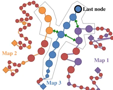
For the approach presented in this paper, a local map consists of the biggest fully connected graph that can be created through neighbor and loop closure links from the last node (used as the root) with those in WM. Figure2.2 illustrates the concept. The diamonds represent initial and end nodes for each mapping session. The nodes in LTM are shown in red and the others are those in WM. The current local map is created and optimized only using nodes in WM that are linked to the last node (all nodes in the dashed area). The local map therefore represents more than the latest mapping session: it can span over multi-session mapping through loop closure links (green links). The other nodes still in WM that are not included in the local map are unreachable from the last node through links available in WM at this time.
Map 1!
Map 2!
Map 3!
Last node!
Figure 2.2 Illustration of a local map created from multi-session mapping.
Using this memory management approach, some parts of the map may be missing for graph optimization, as described in 2.2.2. Online graph optimization is done on the local map, with the constraints available in WM at that time. Constraints transferred to LTM are not used, thus limiting graph quality compared to using all constraints available. This is the compromise to make to be able to satisfy online processing requirements. However, if required, the approach is still able to create a global map by using all constraints from LTM and conduct offline a global graph optimization.
2.3
Results
The data sets used for the experiments are acquired using the AZIMUT-3 robot [Ferland et coll., 2010], shown by Figure2.3, equipped with a URG-04LX laser rangefinder and a Kinect sensor. The RGB images from the Kinect are used for the appearance-based loop closure detection while the depth images are used to find the 3D position of the visual words. Laser scans and RGB-D point clouds created from the Kinect are used for map visualization. As mentioned in 2.2.1, since in this experiment the robot is constrained to a single plane, loop closure transformations are refined using 2D ICP with the laser scans to increase precision: the transformations are then limited to three degrees of freedom (x, y and rotation over z axis), ignoring noise on other degrees of freedom computed by the visual transformation.
Five mapping sessions (total length of 750 m) were conducted by starting the robot at different locations in our lab building. Between the mapping sessions, the robot was turned
2.3. RESULTS 13
Kinect! URG-04LX!
AZIMUT-3!
Figure 2.3 AZIMUT-3 robot equipped with a URG-04XL laser range finder and a Kinect sensor.
off to reset odometry, and moved to another location. In each session, the robot revisited at least one part of the environment mapped in a previous session. Data acquisition is done using the ROS bag mechanism (http://ros.org). Odometry, laser scans, RGB images and depth images are recorded at 1 Hz (i.e., R = 1 s) in a ROS bag. A ROS bag can be played using the same timings as during acquisition, making a realistic input for mapping and a good common format for other algorithms using ROS. One ROS bag per mapping session is taken. The ROS bags are processed on a MacBook Pro 2010: 2.66 GHz Intel Core i7 and SSD hard drive (on which the LTM is saved).
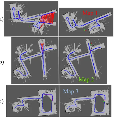
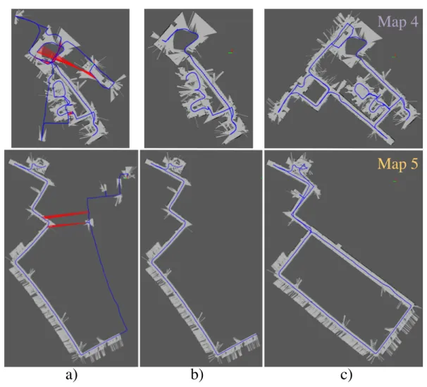
Two experiments were conducted (STM size S = 10, minimum inliers I = 5 of RANSAC, hypothesis threshold H = 0.11 and similarity threshold Y = 0.45). For the first experi-ment, our approach processed each mapping session independently, i.e., the memory was cleared between each session. Time limit T was set to 0.7 s. Figure2.4 shows the result-ing maps for sessions 1, 2 and 3, with and without graph optimizations. The light gray areas are empty spaces detected using the laser rangefinder. No nodes were transferred to LTM in these experiments (local maps are equal to global maps). This is confirmed by Figure2.6: T was never reached for these sessions, and thus all nodes were used for loop closure detection and graph optimization. Figure2.5 shows results for the mapping sessions 4 and 5 (i.e., Map 4 and Map 5): the global graph not optimized (left), the last local map (middle) and the global map (right). The local map is the biggest map that was created online from the last node (with nodes available in WM), and the global map was generated offline after the mapping sessions (with all nodes in WM and LTM). As shown by Figure2.6, T was reached before the end. Figure2.5 b) illustrate the effect of transferring nodes to LTM to satisfy the online requirement. Even if loop closures can be detected with older portions of the map still in WM (as shown in a)), the maps cannot
a)!
b)!
c)!
Map 1!
Map 2!
Map 3!
Figure 2.4 Resulting local maps without (left) and with (right) graph opti-mizations for a) Map 1, b) Map 2 and c) Map 3. Loop closures are shown in red.
be globally optimized if the neighbors of the loop closures are in LTM. For comparison, Figure2.5 c) are maps created offline using all constraints in LTM: here, loop closures with old portions of the map have an effect on graph optimization.
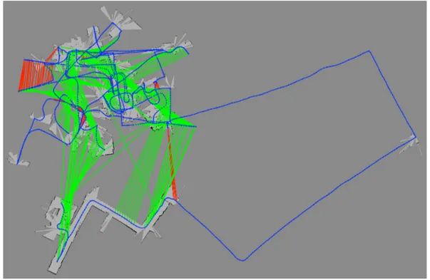
For the second experiment, the data sets for the five maps were processed one after each other, as in a real multi-session mapping trial. The robot automatically started a new map when the odometry was reset to zero before each session. The memory was preserved between the sessions and T was also set to 0.7 s. Figure2.7 shows the last local map (nodes in light gray areas are those in WM) and global graph (blue line) without optimization. The maps lie over each other because they are all starting from the same referential. Loop closures detected in the same map (intra-session) and those detected between the maps (session) are shown in red and green, respectively. To distinguish more easily inter-session loop closures, Figure2.8 illustrates the global graph for y-value of the poses over time. Note that all paths for each session started at y = 0 and they were not connected together by neighbor links. Optimizing the graph using all these detected loop closures results in a single fully connected map of all five mapping sessions. Figure2.9 shows the
2.3. RESULTS 15
a)!
b)!
c)!
Map 4!
Map 5!
Figure 2.5 Results for Map 4 (top) and Map 5 (bottom), with a) the map from all nodes still in WM (light gray) with the global graph (blue line) not optimized, b) the local map with local graph optimization and c) the global map with global graph optimization. Loop closures are shown in red.
resulting global map by assembling the RGB-D point clouds from the Kinect using the optimized poses of the graph.
Figure2.10 a) shows the resulting local map created from all the mapping sessions. Because the local map is built only from nodes in WM that are linked (directly or indirectly) to the last node, only a small portion of the global map is available online. Note that the local map is also smaller than Map 5 taken independently (shown by Figure2.5): in the second experiment, there were nodes with more weight from previous mapping sessions that were still in WM, thus more nodes from the latest mapping session were transferred to LTM and not used for local map creation. These high weighted nodes are located in the light gray areas of Figure2.10 b). The blue line represents the global graph created using all constraints in LTM. When using all constraints in LTM, the local map is also
0 200 400 600 800 0 0.2 0.4 0.6 0.8 1 Node indexes
Time (s) Map 1: 333 nodes
Map 2: 297 nodes Map 3: 207 nodes Map 4: 729 nodes Map 5: 518 nodes
Figure 2.6 Processing time in relation to the number of nodes processed over time for each data set. T is shown by the horizontal line.
Figure 2.7 Top view of the map without optimization after five mapping ses-sions. The red and green links show intra-session and inter-session loop closures detected, respectively.
2.3. RESULTS 17 −10 0 10 20 30 40 50 0 500 1000 1500 2000 2500 y Node indexes
Map 1
Map 2
Map 3
Map 4
Map 5
(m)
Figure 2.8 Loop closures between the mapping sessions. Only the y values of the poses are illustrated for visibility purposes. Green and red links are inter-session and intra-inter-session loop closures detected, respectively. Neighbor links are shown in blue. Note that only green links connect the five maps together.
with all mapping sessions connected, with 330 nodes in WM (107, 12, 27, 28, 156 nodes from maps 1, 2, 3, 4 and 5, respectively) for which 173 nodes are accessible for the local map (4, 15, 6, 0, 148 nodes from maps 1, 2, 3, 4 and 5, respectively). For the local map, it is normal that a high proportion of nodes are from the last session, which is the most recent one. Nodes from older maps are those retrieved from LTM around the latest loop closures found. For example, when the robot is mapping a new area, only nodes of the last session would be in the local map.
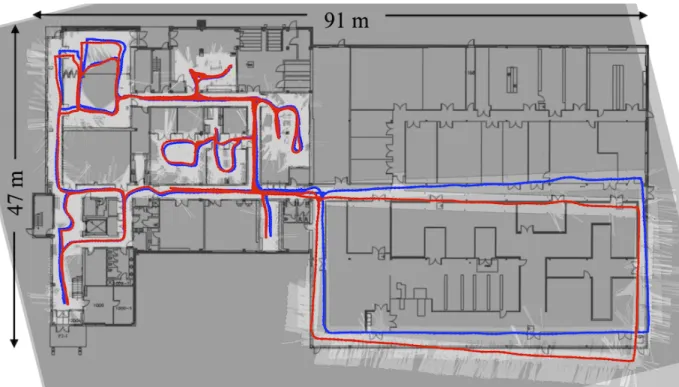
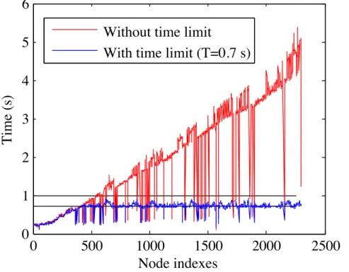
To observe the influence of memory management on the quality of the map created, we conducted the same experiment without T . All nodes were then kept in WM and they were processed by both loop closure detection and graph optimization at each time step. Normally, without transferring nodes to LTM, more loop closures would be detected, so more constraints would be used for graph optimization. As shown in Figure2.12, the processing time becomes greater than the acquisition time R, which is not the case with T = 0.7 s. However, without T , 193 intra-session and 387 inter-session loop closures were detected, comparatively to 188 and 258 respectively for the online experiment. Figure2.11 compares the resulting global maps with (blue) and without (red) T . By comparing with the building plan (the plan was scaled to 5 cm / pixel like the generated maps, the maps were manually oriented so trajectories are aligned to most doors traversed), the quality of the experiment without T (red) is a little better than with T (blue), probably because more loop closures were used for graph optimization. However, for the two conditions, the large loop from Map 5 is not correctly aligned with the building plan. The robot traversed this area only once and exited from the same door from which it entered, making it more difficult for the graph optimization algorithm to correct angular errors for this single entry point. For comparison, the left part of the map was also traversed once during session 4, but the robot exited the area from another door, thus making the area more robust to angular errors.
2.4
Discussion
In term of processing time, the results show that the proposed approach is able to satisfy online processing requirements independently of the size of the environment. However, map quality depends on the number of loop closures that can be detected. To satisfy online requirements, the robot transfers in LTM some portions of the map which cannot be used for loop closure detection. For multi-session mapping, the worst case would occur if all nodes of a previous map are transferred to LTM before a loop closure is detected with the new map. This would result in definitely forgetting the previous map: there
2.4. DISCUSSION 19
a)!
b)!
Figure 2.10 Graphs optimized for a) the last local map built online, b) the global map built offline, with nodes in light gray areas are those still in WM, and the other nodes are in LTM.
Figure 2.11 Global maps with (blue) and without (red) T . The maps are manually superimposed over the actual plan of the building.
would be no links in WM and even in LTM that could connect this older map to the new one, and it would be ignored even for the global map construction. To avoid this problem, our approach could keep at least one node for each map in WM. However, if the number
0
500
1000
1500
2000
2500
0
1
2
3
4
5
6
Node indexes
Time (s)
Without time limit
With time limit (T=0.7 s)
Figure 2.12 Processing time for each node added to graph. The horizontal lines are T = 0.7 and R = 1.
of mapping sessions becomes very high (e.g., thousands of sessions), these nodes would definitely have to be transferred in LTM to satisfy the online requirement. For long-term, large-scale and multi-session mapping, some portions of the map would then be definitely forgotten, and therefore some kind of heuristic to efficiently manage important nodes to keep in WM is required.
Another observation is that frequently revisiting old maps increases global map quality. A robot autonomously mapping a facility could, when detecting an old map, decide to revisit some parts of it to detect more inter-session loop closures, thus creating more constraints for graph optimization.
In the experiments conducted, no invalid loop closures were detected. If this occur, erro-neous constraints would be added to graph optimization, resulting in map errors. Some graph optimization approaches such as [Latif et coll., 2012; Sunderhauf et Protzel, 2012] deal with possible invalid matches, and could be used to increase robustness of the pro-posed approach.
2.5. CONCLUSION 21
2.5
Conclusion
Results presented in this paper suggest that the proposed graph-based SLAM approach is able to meet online requirements needed for large-scale, long-term and multi-session online mapping. By limiting the number of nodes in WM available for global loop closure detection and graph optimization, online processing is achieved for new data acquired. Our approach is tightly based on global loop closure detection, allowing it to naturally deal with the kidnapped robot problem and gross errors in odometry. Our code is open source and available at http://introlab.github.io/rtabmap/. In future work, we plan to study the impact of autonomous exploration strategies on multi-session mapping, especially how it can actively direct exploration based on nodes available for online mapping and graph optimization.
CHAPITRE 3
Long-Term Online Multi-Session Graph-Based
SPLAM with Memory Management
Avant-propos
Auteurs et affiliations :M. Labbé : étudiant au doctorat, Université de Sherbrooke, Faculté de génie, Dépar-tement de génie électrique et de génie informatique.
F. Michaud : professeur, Université de Sherbrooke, Faculté de génie, Département de génie électrique et de génie informatique.
Date d’acceptation :6 novembre 2017
État de l’acceptation :version finale publiée en août 2018, volume 42, numéro 6 (https: //doi.org/10.1007/s10514-017-9682-5).
Revue : Autonomous Robots
Référence :[Labbé et Michaud, 2017]
Titre français :Planification, localisation et cartographie simultanées ‘en ligne’ et à long terme avec gestion de mémoire
Contribution au document :Cet article contribue à la thèse en élaborant comment la gestion de mémoire peut être intégrée à un robot faisant continuellement du SLAM tout en navigant de façon autonome. Le défi est d’avoir assez d’information dans la mémoire de travail du robot pour correctement suivre une trajectoire planifiée tout en étant capable de se relocaliser globalement sur une longue période d’opération, et ce, toujours en effectuant le traitement ‘en ligne’.
Résumé français : Pour la planification, la localisation et la cartographie simultanées à long terme (SPLAM), un robot doit pouvoir mettre continuellement à jour sa carte en fonction des changements dynamiques de l’environnement et des nouvelles zones explorées. Avec des capacités de calcul embarquées limitées, un robot doit également pouvoir limiter la taille de la carte utilisée pour que la localisation et la cartographie soient toujours possible
par du traitement ‘en ligne’. Cet article aborde ces défis en utilisant un mécanisme de gestion de mémoire qui identifie les endroits qui doivent rester dans une mémoire de travail (WM) pour être traités ‘en ligne’, et à ceux qui doivent être transférés vers une mémoire à long terme (LTM). Lorsque des endroits précédemment transférés dans la LTM sont revisités, le mécanisme de gestion de mémoire peut récupérer ces endroits et les replacer dans la WM pour être utilisés par le SPLAM. L’approche est testée sur un robot équipé d’un télémètre laser à courte portée et d’une caméra RGB-D, patrouillant de manière autonome un total de 10,5 km dans un environnement intérieur sur 11 sessions tout en ayant rencontré 139 personnes.
3.1. INTRODUCTION 25
Abstract
For long-term simultaneous planning, localization and mapping (SPLAM), a robot should be able to continuously update its map according to the dynamic changes of the environ-ment and the new areas explored. With limited onboard computation capabilities, a robot should also be able to limit the size of the map used for online localization and mapping. This paper addresses these challenges using a memory management mechanism, which identifies locations that should remain in a Working Memory (WM) for online processing from locations that should be transferred to a Long-Term Memory (LTM). When revisiting previously mapped areas that are in LTM, the mechanism can retrieve these locations and place them back in WM for online SPLAM. The approach is tested on a robot equipped with a short-range laser rangefinder and a RGB-D camera, patrolling autonomously 10.5 km in an indoor environment over 11 sessions while having encountered 139 people.
3.1
Introduction
The ability to simultaneously map an environment, localize itself in it, and plan paths using this information is known as Simultaneous Planning, Localization And Mapping, or SPLAM [Stachniss, 2009]. This task can be particularly complex when done online on a robot with limited computing resources in large, unstructured and dynamic environments. Since SPLAM can be seen as an extension of Simultaneous Localization And Mapping (SLAM), many approaches exist [Thrun et coll., 2005]. Our interest lies with graph-based SLAM approaches [Grisetti et coll., 2010], for which combining a lightweight topological map over a detailed metrical map reveals to be more suitable for large-scale mapping and navigation [Konolige et coll., 2011].
Two important challenges in graph-based SPLAM are :
– Multi-session mapping, also known as the kidnapped robot problem or the initial state problem: when turned on, a robot does not know its relative position to a map previously created, making it impossible to plan a path to a previously visited location. A solution is to have the robot localize itself in a previously-built map before initiating mapping. This solution has the advantage of always using the same referential, resulting in only one map is created across the sessions. However, the robot must start in a portion already mapped of the environment. Another approach is to initialize a new map with its own referential on startup, and when a previously visited location is encountered, a transformation between the two maps can be computed. The transformations between the maps can be saved explicitly
with special nodes called anchor nodes [Kim et coll., 2010; McDonald et coll., 2012], or implicitly with links added between each map [Konolige et Bowman, 2009; Latif et coll., 2013]. This process is referred to as loop closure detection. Loop closure detection approaches that are independent of the robot’s estimated position [Ho et Newman, 2006] can intrinsically detect if the current location is a new location or a previously visited one among all the mapping sessions conducted in the past. Popular loop closure detection approaches are appearance-based [Garcia-Fidalgo et Ortiz, 2015], exploiting the distinctiveness of images of the environment. The underlying idea is that loop closure detection is done by comparing all previous images with the new one. When loop closures are found between the maps, a global map can be created by combining the maps from each session. In graph-based SLAM, graph pose optimization approaches [Folkesson et Christensen, 2007; Grisetti et coll., 2007a; Johannsson et coll., 2013; Kummerle et coll., 2011] use these loop closures to reduce odometry errors inside each map and in between the maps.
– Long-term mapping in dynamic environments. Persistent [Milford et Wyeth, 2010], lifelong [Konolige et Bowman, 2009] or continuous [Pirker et coll., 2011] are terms generally used to describe SLAM approaches working in such conditions. Continu-ously updating and adding new data to the map in unbounded or dynamic environ-ments will inevitably increase the map size over time. Online simultaneous planning, localization and mapping requires that new incoming data be processed faster than the time to acquire them. For example, if data are acquired at 1 Hz, updating the map should be done in less than 1 sec. As the map grows, the time required for loop closure detection and graph optimization increases, and eventually limits the size of the environment that can be mapped and used online.
To address these challenges, we introduce SPLAM-MM, a graph-based SPLAM with a memory management (MM) mechanism. As demonstrated in [Labbé et Michaud, 2013], memory management can be used to limit the size of the map so that loop closure detec-tions are always processed under a fixed time limit, thus satisfying online requirements for long-term and large-scale environment mapping. The idea behind SPLAM-MM is to limit the number of nodes available for loop closure detection and graph optimization, keeping enough observations in the map for successful online localization and planning while still having the ability to generate a global representation of the environment that can adapt to changes over time.
The paper is organized as follows. Section 3.2 reviews graph-based SLAM approaches that reduce the size of the map when revisiting the same environment while continuously
3.2. RELATED WORK 27 adapting to dynamic changes. Section 3.3 describes the implementation and the operating principles associated with the use of memory management with a graph-based SPLAM approach, which extends our previous metric-based SLAM approach [Labbé et Michaud, 2014] with a new planning capability. The implementation integrates four algorithms: loop closure detection [Labbé et Michaud, 2013], graph optimization [Grisetti et coll., 2007a], metrical path planner [Marder-Eppstein et coll., 2010] and a custom topological path planner. Section 3.4 presents experimental results of 11 SPLAM sessions using the AZIMUT-3 robot in an indoor environment over 10.5 km. Section 3.5 discusses strengths and limitations of SPLAM-MM, and Section 3.6 concludes the paper.
3.2
Related Work
Lifelong appearance-based SLAM requires dealing with dynamic environments. [Glover et coll., 2010] present an appearance-based SLAM approach that had to operate in different lighting conditions over three weeks. An interesting observation from their experiments is that even when revisiting the same locations, the map still grows: in dynamic environ-ments, the loop closure detector is sometimes unable to detect loop closures, duplicating locations in the map. A map management approach is therefore required to limit map size. In highly dynamic environments, multiple views of the same location may also be re-quired for proper localization. [Churchill et Newman, 2012] present a graph-based SLAM approach where visual experiences of the same locations are kept in the map, to increase localization robustness to dynamic changes caused for instance by outdoor illumination conditions. If localization fails when revisiting an area, new experiences are added to the map. Even if adding new visual experiences to the map happens less often over time (as the robot explores the same location), there is no mechanism to limit this. [Pirker et coll., 2011] present a continuous monocular SLAM approach where new key frames are added to the map only when the environment has changed, to keep its size proportional to the explored space. But if the environment changes very often, there is no mechanism to limit the number of key frames over the same physical location.
Some SLAM approaches can handle dynamic changes of the environment while limiting the size of the map for long-term operation. [Biber et Duckett, 2005] present a sample-based representation for maps, to handle changes at different timescales, tracking both stationary and non-stationary elements of the environment. The idea is to refresh samples stored for each timescale with new sensor measurements. Map growth is then indirectly limited as older memories fade at different rates depending on the timescale. [Walcott-Bryant et coll., 2012] describe Dynamic Pose-Graph SLAM (DPG-SLAM), a long-term mapping
approach that detects static and dynamic changes of the environment through time. To keep consistency of the graph while reducing its size, nodes that are not observable anymore are removed. [Johannsson et coll., 2013] also remove unobservable nodes to limit the size of the map over time when revisiting the same area. Similar nodes of the graph are merged together while keeping only the new loop closure detection. However, the graph size is not bounded when exploring new areas. [Krajník et coll., 2016] present an occupancy grid approach where each cell in the map estimates its occupancy value depending on periodical and cyclic changes occurring in the environment. This increases localization and navigation accuracy in dynamic environments compared to static maps, as the predicted map represents the correct state of the environment at that time of the day (e.g., doors can change to be opened or closed). The maximum data kept for each cell is bounded by some parameters (depending on the smallest and longest cyclic periods that should be detected), thus keeping memory usage fixed. However, the approach assumes that the navigation phase always occur in the same environment as the first mapping cycle, without possibility to extend it afterward.
These problems of lifelong SLAM are also addressed in some SPLAM approaches. [Milford et Wyeth, 2010] present a solution to limit the size of the map (called experience map) while revisiting the same area: close nodes are merged together up to a maximum density threshold. This approach has the advantage of making the map size independent of the operating time, but the diversity of the observations on each location is somewhat lost. [Konolige et coll., 2011] use a view-based graph SLAM approach [Konolige et Bowman, 2009] in a SPLAM context. The approach preserves diversity of the images referring to the same location so that the map can handle dynamic changes over time, and forgetting images limits the size of the graph over time when revisiting the same area. However, the graph still grows when visiting new areas.
Overall, these approaches reduce map size when revisiting the same area, while continu-ously adapting to dynamic changes. This makes them independent or almost independent of the operation time of the robot in these conditions, but they are all limited to a max-imum size of the environment that can be mapped online. The SPLAM-MM approach deals specifically with this limitation.
3.3
Memory Management for SPLAM
The underlying representation of SPLAM-MM is a graph with nodes and links. The nodes contain the following information:
3.3. MEMORY MANAGEMENT FOR SPLAM 29
Figure 3.1 The AZIMUT-3 robot equipped with a URG-04LX laser range finder and a Xtion PRO LIVE sensor.
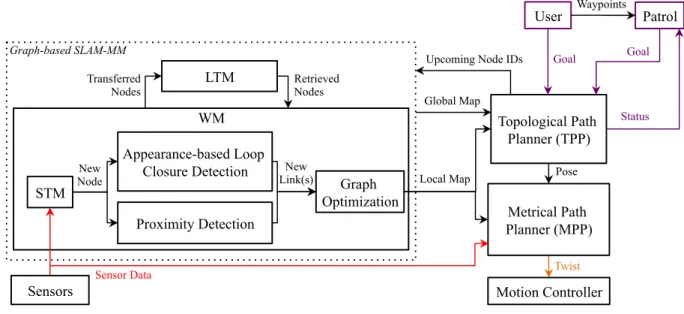
Motion Controller Waypoints Graph-based SLAM-MM WM STM SPLAM-MM Graph-based SLAM-MM Wheel Odometry Laser Rangefinder RGB-D Camera Motion Controller Topological Path Planner (TPP) Twist Pose Scan RGB-D Image Local Map
Upcoming Node IDs
Metrical Path Planner (MPP) Pose User Goal Appearance-based Loop Closure Detection Graph Optimization New Link(s) New
Node Local Map
Proximity Detection Sensor Data Sensors Global Map LTM Transferred
Nodes Retrieved Nodes
Global Map Upcoming Node IDs
Patrol Goal Status Waypoints Topological Path Planner (TPP) Twist Metrical Path Planner (MPP) Pose User Goal Patrol Goal Status
Figure 3.2 Memory management and control architecture of SPLAM-MM. – ID: unique time index of the node.
– Weight: an indication of the importance of the node, used for memory management. – Bag-of-words (BOW): visual words used for loop closure detections. They are SURF features [Bay et coll., 2008] quantized to an incremental vocabulary based on KD-Trees.
– Sensor data: used to find similarities between nodes and to construct maps. For this paper, our implementation of SPLAM-MM is using the AZIMUT-3 robot [Ferland et coll., 2010], equipped with an URG-04LX laser rangefinder and a Xtion Pro Live RGB-D camera, as shown by Figure 3.1. The sensory data used are:
– Pose: the position of the robot computed by its odometry system (e.g., the value given by wheel odometry), expressed in (x, y, θ) coordinates.
– RGB image: used to extract visual words.
– Depth image: used to find 3D position of the visual words. The depth image is registered with the RGB image, i.e., each depth pixel corresponds exactly to the same RGB pixel.
– Laser scan: used for loop closure transformations and odometry refinements, and by the Proximity Detection module.
The links store rigid transformations (i.e., Eucledian transformation derived from odom-etry or loop closures) between nodes. There are four types of links:
– Neighbor link: created between a new node and the previous one.
– Loop closure link: added when a loop closure is detected between the new node and one in the map.
– Proximity link: added when two close nodes are aligned together.
– Temporary link: used for path planning purposes. It is used to keep the planned path connected to the current map.
Figure 3.2 presents a high-level representation of SPLAM-MM. Basically, it consists of a graph-based SLAM module with memory management, to which path planners are added. Memory management involves the use of a Working Memory (WM) and a Long-Term Memory (LTM). WM is where maps, which are graphs of nodes and links, are processed. To satisfy online constraints, nodes can be transferred and retrieved from LTM. More specifically, the WM size indirectly depends on a fixed time limit T : when the time required to update the map (i.e., the time required to execute the processes in the Graph-based SLAM-MM block) reaches T , some nodes of the map are transferred from WM to LTM, thus keeping WM size nearly constant and processing time around T . However, when a loop closure is detected, neighbors in LTM with the loop closure node can be retrieved from LTM to WM for further loop closure detections. In other words, when a robot revisits an area which was previously transferred to LTM, it can incrementally retrieve the area if a least one node of this area is still in WM. When some LTM nodes are retrieved, nodes in WM from other areas in the map can be transferred to LTM, to limit map size in WM and therefore keeping processing time around T .
Therefore, the choice of which nodes to keep in WM is key in SPLAM-MM. The objective is to have enough nodes in WM from each mapping session for loop closure detections and to keep a maximum number of nodes in WM for generating a map usable to follow
3.3. MEMORY MANAGEMENT FOR SPLAM 31 correctly a planned path, while still satisfying online processing. Two heuristics are used to establish the compromise between selection of which nodes to keep in WM and online processing:
– Heuristic 1 is inspired from observations made by psychologists [Atkinson et Shiffrin, 1968; Baddeley, 1997] that people remember more the areas where they spent most of their time, compared to those where they spent less time. In terms of memory management, this means that the longer the robot is at a particular location, the larger the weight of the corresponding node should be. Oldest and less weighted nodes in WM are transferred to LTM before the others, thus keeping in WM only the nodes seen for longer periods of time. As demonstrated in [Labbé et Michaud, 2013], this heuristic reveals to be quite efficient in establishing the compromise between search time and space, as driven by the environment and the experiences of the robot.
– Heuristic 2 is used to identifies nodes that should stay in WM for autonomous navigation. Nodes on a planned path could have small weights and may be identified for transfer to LTM by Heuristic 1, thus eliminating the possibility of finding a loop closure link or a proximity link with these nodes and correctly follow the path. Therefore, Heuristic 2 must supersede Heuristic 1 and allow upcoming nodes to remain in WM, even if they are old and have a small weight.
The Graph-based SLAM-MM block provides two types of maps derived from nodes in WM and LTM:
– Local map, i.e., the largest connected graph that can be created from the last node in WM with nodes available in WM only. The local map is used for online path planning.
– Global map, i.e., the largest connected graph that can be created from the last node in WM with nodes in WM and LTM. It is used for offline path planning.
Figure 3.3 uses diamonds to represent initial and end nodes for each mapping session. The nodes in LTM are shown in red and the others are those in WM. The local map is created using only the nodes in WM that are linked to the last node. The graph linking the last node with other nodes in WM and LTM represents the global map (outer dotted area). If loop closure detections are found between nodes of different maps, loop closure links can be generated, and the local map can span over multiple mapping sessions. Other nodes in WM but not included in the local map are unreachable from the last node, but they are
Map 1!
Map 3!
Map 4!
Last node!
Map 2!
Local map!
Global map!
Figure 3.3 Illustration of the local map (inner dashed area) and the global map (outer dotter area) in multi-session mapping. Red nodes are in LTM, while all other nodes are in WM. Loop closure links are shown using bidirectional green arrows.
still used for loop closure detections since all nodes in WM (including those in Map 2 for instance) are examined.
The modules presented in Figure 3.2 are described as follows.
3.3.1
Short-Term Memory Module
Short-Term Memory (STM) is the entry point where sensor data are assembled into a node to be added to the map. Similarly to [Labbé et Michaud, 2013], the role of the STM module is to update node weight based on visual similarity. When a node is created, a unique time index ID is assigned and its weight is initialized to 0. The current pose, RBG image, depth image and laser scan readings are also memorized in the node. If two consecutive nodes have similar images, i.e., the ratio of corresponding visual words between the nodes is over a specified threshold Y , the weight of the previous node is increased by one. If the robot is not moving (i.e., odometry poses are the same), the new node is deleted. To reduce odometry errors on successive STM nodes, transformation refinement is done using 2D iterative-closest-point (ICP) optimization [Besl et McKay, 1992] on the rigid transformation of the neighbor link with the previous node and the corresponding laser scans. If the ratio of ICP point correspondences between the laser scans over the
3.3. MEMORY MANAGEMENT FOR SPLAM 33 total laser scan size is greater or equal to C, the neighbor link’s transformation is updated with the correction.
When the STM size reaches a fixed size limit of S nodes, the oldest node in STM is moved to WM. STM size is determined based on the velocity of the robot and at which rate the nodes are added to the map. Images are generally very similar to the newly added node, keeping S nodes in STM avoids using them for appearance-based loop closure detection once in WM. For example, at the same velocity, STM size should be larger if the rate at which the nodes are added to map increases, in order to keep nodes with consecutive similar images in STM. Transferring nodes with images very similar with the current node from STM to WM too early limits the ability to detect loop closures with older nodes in WM.
3.3.2
Appearance-based Loop Closure Detection Module
Appearance-based loop closure detection is based on the bag-of-words approach described in [Labbé et Michaud, 2013]. Briefly, this approach uses a bayesian filter to evaluate appearance-based loop closure hypotheses over all previous images in WM. When a loop closure hypothesis reaches a pre-defined threshold H, a loop closure is detected. Visual words of the nodes are used to compute the likelihood required by the filter. In this work, the Term Frequency-Inverse Document Frequency (TF-IDF) approach [Sivic et Zisserman, 2003] is used for fast likelihood estimation, and FLANN (Fast Library for Approximate Nearest Neighbors) incremental KD-Trees [Muja et Lowe, 2009] are used to avoid rebuild-ing the vocabulary at each iteration. To keep it balanced, the vocabulary is rebuilt only when it doubles in size.
The RGB image, from which the visual words are extracted, is registered with a depth image. Using (3.1), for each 2D point (x, y) in the rectified RGB image, a 3D position Pxyz
can be computed using the calibration matrix (focal lengths fx and fy, optical centres cx
and cy) and the depth information d for the corresponding pixel in the depth image. The
3D positions of the visual words are then known. When a loop closure is detected, the rigid transformation between the matching images is computed using a RANSAC (RANdom SAmple Consensus) approach which exploits the 3D visual word correspondences [Rusu et Cousins, 2011]. If a minimum of I inliers are found, the transformation is refined using the laser scans in the same way as the odometry correction in STM using 2D ICP transformation refinement. If transformation refinement is accepted, then a loop closure link is added with the computed transformation between the corresponding nodes. The weight of the current node is updated by adding the weight of the loop closure hypothesis