The economics of US greenhouse gas emissions reduction policy : assessing distributional effects across households and the 50 United States using a recursive dynamic computable general equilibrium (CGE) model

The Economics of US Greenhouse Gas Emissions Reduction Policy: Assessing Distributional Effects Across Households and the 50 United States Using a Recursive Dynamic Computable General Equilibrium (CGE) Model

by

Wesley Allen Look

BA English Wesleyan University Middletown, Connecticut (2002)

SUBMITTED TO THE DEPARTMENT OF URBAN STUDIES AND PLANNING IN PARTIAL FULFILLMENT OF THE REQUIREMENTS FOR THE DEGREE OF

MASTER OF SCIENCE AT THE

MASSACHUSETTS INSTITUTE OF TECHNOLOGY FEBRUARY 2013

0 2013 Wesley Look. All Rights Reserved.

The author hereby grants to MIT the permission to reproduce and to distribute publicly paper and electronic copies of the thesis document in whole or in part in any medium now known or hereafter created.

Author

Certified by

7,-71"

Accepted by_

D(partient of Urban Studies and Planning /-A Oc 15, 2012

Professor Lawrence Susskind Department of Urban Studies and Planning Thesis Supervisor

Professor Alan Berger Committee Chair Department of Urban Studies and Planning

1

, I

The Economics of US Greenhouse Gas Emissions Reduction Policy: Assessing the Distributional Effects Across Households and the 50 United States

Using a Recursive Dynamic Computable General Equilibrium (CGE) Model by

Wesley Allen Look

Submitted to the Department of Urban Studies and Planning on October 15, 2012 in Partial Fulfillment of the Requirements for the Degree of Master of Science in Urban Studies and Planning

Abstract

The political economy of US climate policy has revolved around state- and district- level distributional economics, and to a lesser extent household-level distribution questions. Many politicians and analysts have suggested that state- and district-level climate policy costs (and their distribution) are a function of local carbon intensity and commensurate electricity price sensitivity. However, other studies have suggested that what is most important in determining costs is the means by which revenues from a price on carbon are allocated. This is one of the first studies to analyze these questions simultaneously across all 50 United States, household income classes and a timeframe that reflects most recent policy proposals (2015 - 2050). I use a recursive dynamic computable general equilibrium (CGE) model to estimate the economic effects of a US "cap-and-dividend" policy, by simulating the implementation of the Carbon Limits and Energy for America's Renewal (CLEAR) Act, a bill proposed by Senators Cantwell (D-WA) and Collins (R-ME) in 2009. I find that while carbon intensity and electricity prices are indeed important in determining compliance costs in some states, they are only part of the story. My results suggest that revenue allocation mechanisms and new investment trends related to the switch to low-carbon

infrastructure are more influential than incumbent carbon intensity or electricity price impacts in determining the distribution of state-level policy costs. These findings suggest that the current debate in the United States legislature over climate policy, and the constellation of both supporters and dissenters, is based upon an incomplete set of assumptions that must be revisited. Finally, please note that this study does not claim to comprehensively model the CLEAR Act,. nor does it incorporate a number of important data and assumptions, including: the latest data on natural gas resources and prices, the price effects on coal of EPA greenhouse gas and mercury regulations, the most recent trends in renewable energy pricing.

Thesis Supervisor: Lawrence Susskind

1. Introduction

Efforts to establish nationwide greenhouse gas reduction policies in the United States have failed largely due to disagreement over the scale of economic burden that such policies might create, and over who would bear the brunt of this burden. For example, among coal-rich states there has been concern that economic costs would fall unequally on their shoulders, while less carbon intensive states would be relatively unhindered. Others (e.g. Orszag (2007) and Greenstein (2007)) have cautioned that economic impacts could disproportionately hit low-income households, which annually spend a larger percentage of total income on non-luxury goods, such as home energy and transportation-both of which are predicted

to rise in price due to an emissions abatement policy. While a number of studies have explored these questions, few have done so in a way that reflects the full political economy of US climate policy-namely at the level of states and congressional districts and across the 30-40 year timeline characteristic of most climate policy proposals. This paper adds some of this detail to the discussion, by modeling the distributional economics of a recent climate policy proposal across the 50 states and from 2006 to 2050.

The debate over climate policy in the US Congress extends at least as far back as the late 1970s, when the first hearings on the topic were held in the House of Representatives (Kamarck 2010). In the early years, there was little disagreement over the science or economics of climate change, partly because at that time Congress was only considering modest policy actions, such as funding research (Keller 2009). Trenchant debate over the economic costs and benefits of policies to reduce greenhouse gas emissions did not begin until the 1990s. In 1997, the Byrd-Hagel "Sense of the Senate" Resolution opposing the ratification of the Kyoto Protocol stated that "emission reductions could result in serious harm to the United States

economy, including significant job loss, trade disadvantages, increased energy and consumer costs, or any combination thereof' (Selin and VanDeveer 2011). The resolution went on to proclaim that the Senate should not be a signatory to any agreement that "would result in serious harm to the economy of the United States," and that any proposed emissions reduction agreement or policy "should also be accompanied by an analysis of the detailed financial costs and other impacts on the economy of the United States" (1 05*h Congress, Senate Res. 98). These declarations announced the deep concern of the US Congress about the economic impacts of a policy to reduce domestic greenhouse gas emissions; they also underscored the need for a clearer understanding of such impacts.

Concern over the economics of a policy to reduce greenhouse gas emissions in the US also includes a question of distributional effects, or the ways in which economic output or welfare is allocated among different parts of the economy. The primary domain of distributional economics refers to individuals or households across income classes. A central focus of this discourse is to determine whether a policy is

progressive or regressive-whether the policy disproportionately benefits (progressive) or burdens (regressive) low-income groups, who are the least able to cope with additional economic costs. For example, in 2007, the House Budget Committee held a hearing entitled Counting the Change: Accounting for the Fiscal Impacts of Controlling Carbon Emissions, which focused on this question in great detail.

Testimony from individuals such as Robert Greenstein explained that "[t]he policies needed to reduce greenhouse gas emissions would, by themselves, result in regressive changes in energy prices. But they also can generate substantial revenue that could be used to offset those regressive impacts" (Greenstein 2007). As Greenstein's statement concisely acknowledges, there is a relatively well-understood remedy for undesirable distributional impacts in the context of climate policy-the requirement that emissions permits be auctioned to generate revenue (which can also be accomplished by a carbon tax), and that these revenues be used to counteract regressivity. This continues to be an important concern in debates about the formulation of climate policy in the United States.

Another crucial sphere of the distributional economics of US climate policy deals with the allocation of welfare across the 50 United States. Palmer et al (2012) estimate that the economic burden of a carbon tax would indeed fluctuate significantly across the regions of the country. They explain that the largest increase in electricity prices would be felt by the "most coal-intensive regions ...[b]ecause coal is more C02-intensive than other generation fuels" (Palmer et al 2012). Numerous studies have shown that this difference in C02-intesity has important political significance for climate legislation. For example, Holland et al (2011) show a strong correlation between congressional voting patterns and the extent to which a member's home district benefits economically from alternative vehicle CO2 emissions reduction policies. Cragg et al (2012) find a similar correlation between congressional voting patterns and the per-capita greenhouse gas emissions of a congressional member's jurisdiction. Using historical voting results from both the House and the Senate and controlling for representatives' ideology, Cragg et al show that members from districts or states with high per-capita carbon emissions are less likely to vote for policies to reduce greenhouse gas emissions or promote clean energy. Alternatively, they find that members from

districts or states with low per-capita carbon emissions have on average supported legislative efforts to cut emissions. They are explicit about the connection between per-capita CO2 levels and the level of

"regulatory compliance costs." Indeed they use CO2 levels as a proxy for the "price" each region would pay for the enactment of a climate policy (with, of course, higher concentrations of CO2 correlated with

higher costs). Cragg et al connect these findings with the longstanding political economic theory that both "price" and "self-interest" are key determinants of voting behavior (Peltzman 1984). These results suggests that congressional representatives see their local carbon intensity as a determinant of whether and to what extent their constituents will benefit or pay for a climate policy. My research attempts to shed

light on these distributional questions by modeling both household and state distributional impacts of a proposed policy to reduce US greenhouse gas emissions.

2. Review of Literature on the Distributional Effects of US Climate Policy

A number of studies have approached these questions of incidence and efficiency, advancing the policy dialogue in Washington. Below is a brief summary of some of the studies undertaken thus far.

Metcalf (1999) and Dinan and Rogers (2002) address questions of economic efficiency and distributional progressivity associated with the implementation of a group of environmental taxes (Metcalf) and a CO2 allowance scheme (Dinan and Rogers). Both studies make the important point that the allocation of revenues generated from a given policy (either from a tax on carbon or the sale of carbon emissions allowances) largely determines whether such policies are regressive or progressive, finding that carbon pricing alone is regressive. However, both studies show that such policies become progressive when they incorporate revenue allocation schemes that either reduce existing taxes (e.g. payroll taxes or income taxes) or provide flat rate lump-sum rebates to households. Both studies include detail on household

income classes (deciles in Metcalf and quintiles in Dinan and Rogers) and both investigate a range of revenue allocation schemes, however there is no temporal or regional characterization.

Metcalf (2008 and 2007), Burtraw et al (2009) and Rausch et al (2009) present similar findings; namely, that significant progressivity can be achieved with carbon-pricing policies that either reduce other taxes, provide a lump-sum transfer or expand the Earned Income Tax Credit (EITC) program. These studies add regional detail of the United States, however the granularity is limited-Metcalf (2008 and 2007) utilize a 9-region format, while Burtraw et al (2009) and Rausch et al (2009) aggregate individual states into 11 and 12 regions respectively. This allows for some comparison of the policy-induced changes in household

income across broad regions; however the impact on individual states is not elucidated. Metcalf (2008 and 2007) and Burtraw et al (2009) show minimal geographic variation in economic impacts on the average household-although Burtraw et al (2009) does show notable differences between regions for low-income households-while Rausch et al (2009) show significant variation among regions. Specifically, the Rausch results indicate that Midwestern and Southern areas will bear the highest economic costs of a carbon-pricing policy, which the authors attribute to more carbon intensive energy consumption and production patterns in those states. All four of these studies utilize "static" methods to estimate policy impacts-they model a single year, they do not show the progression of economic effects over time.

Hassett et al (2009) analyze household welfare impact associated with the implementation of a CO2 tax. They add a temporal dimension (1987, 1997 and 2003) to the regional (9 regions) and class (deciles) detail of the above studies. They find that the direct impact of a CO2 tax is regressive, while indirect

effects are more proportional-suggesting that a carbon tax is "far less regressive than is generally assumed" (Hassett et al 2009), even without progressive revenue allocation measures such as reducing payroll taxes or offering a lump-sum return. The same study finds that any regressivity is reduced when lifetime income is used as the measure of welfare in place of annual income. Finally, they show little variation in welfare impacts across regions, and that whatever variation does occur diminishes over time.

Rausch et al (2010) look at the distributional impacts of a number of recent CO2 reduction policy proposals in the United States (including the American Clean Energy and Security Act (ACES) of 2009 and the Carbon Limits and Energy for America's Renewal (CLEAR) Act).' The authors employ a

computable general equilibrium model of the US economy with the same core structure used by Rausch et al (2009) (including the 12-region geographic aggregation). The main change from their earlier work is the incorporation of a recursive dynamic component to the model, which allows the authors to include significantly more temporal detail (2006 - 2050, in five year increments after 2010). The study produces similar distributional results to the studies mentioned above, i.e., that all policies with progressive allocation schemes come out as progressive overall. The study shows that negative welfare impacts (as measured by a change in household income) increase over time, as the carbon price increases due to a stricter limit on the quantity of emissions allowed in the economy. The authors show only minimal differences in welfare impacts among regions, and that these relative differences persist over time. That said, there is one major outlier, which experiences much larger welfare changes than other regions. Interestingly, this outlier is one of the few single-state regions, Alaska. The authors-with laudable transparency-point out that Alaska's extreme result is indicative of possible state-by-state differences that are muted by the aggregation of multiple states into single regions. For example, the "Mountain"

region groups together eight states surrounding the Rocky Mountains. This group includes Idaho, which generated about 94 percent of its electricity in 2006 from carbon-neutral hydro and wind resources, and Wyoming, which derived roughly the same percentage (95 percent) of its total 2006 electricity from carbon intensive coal. Together, these two extreme cases effectively neutralize each other. This is a stark example of the obscuring affects that can occur with regional aggregation.

Palmer et al (2012) adds more regional detail than previous studies, but with slightly less temporal detail (2010 - 2035 in five year increments) than the Rausch et al (2010) study. Palmer et al analyze the 1 Please see Section 4 for a brief description of ACES and CLEAR.

variability of revenue generation from a carbon tax, as part of the federal deficit reduction discussion. The authors note that a large share of revenues from such a tax would necessarily come from the electricity sector. This presents regional distributional challenges, since the 50 states are very diverse in terms of electricity generation mix and since this diversity will create variation in how incidence is distributed. As mentioned above, the study shows that states with carbon intensive electricity (e.g. in the Midwest) will pay more than states with relatively low-carbon sources (the Northeast and West Coast). The goal of this study is not to provide a detailed distributional analysis, and therefore it does not account for factors such as revenue recycling-which is somewhat a function of looking at a carbon tax as a deficit reduction measure. While the study provides richer geographic granularity than previous studies, it uses the electricity market modules created by the Energy Information Administration's Annual Energy Outlook, which does not map neatly to state borders.

Boyce and Riddle (2009) estimate the economic impacts of the "cap-and-dividend" policy framework characterized by the Cantwell-Collins CLEAR Act. The authors fully disaggregate the US to its 50 constituent parts and analyze household distributional impacts at both national and state levels. They show, as above, the regressivity of carbon pricing alone, and a progressive turnaround with the inclusion of a the lump-sum rebate or "dividend" mechanism. Indeed, they find the policy as a whole to be strongly progressive at both state and national levels, due to the fact that a uniform dividend (the same dollar amount is given to all households, regardless of income) is of greater value to low-income households than upper-income groups as a percentage of annual income. The authors find this balancing effect to be so strong that low-income households gain more in dividends than they loose in higher energy prices, experiencing a positive net impact. The study shows this same distributional principle, which occurs most prominently at the household level, playing-out at the state level-where poor states disproportionately suffer from the stand-alone carbon price (regressivity) and gain from the dividend mechanism.2

Finally, the authors find that differences in policy-induced welfare impacts are much greater across income groups than across states-showing minimal variation from state to state. Like many of the above papers, this study uses a static analysis-meaning, it only views policy results for a single year (2003).

These many studies addressing the distributional impacts of a range of policies to reduce US greenhouse gas emissions form the foundation for this thesis. Of equal importance are the studies that have helped to elucidate the political economy of CO2 regulation in the United States-namely, that the state and district

2 NB: Theses pains and gains are also a function of the carbon _{intensity of each state, and so there is not an equally}

lucid picture of this trend as in the case of households-which are analyzed either within the same state or across the national energy mix.

level economic impacts of such policy will have great, if not primary, significance in shaping the results of future legislative efforts (Holland et al 2011; Cragg et al 2012). This paper builds on these efforts, by modeling the impacts of a US cap-and-dividend policy, the CLEAR Act, at the level of the 50 states and across the full time dimension of most policy proposals - from 2015 to the year 2050.

3. Model Background and Assumptions

The basis for this study is a recursive dynamic computable general equilibrium (CGE) model of the United States economy designed specifically to study climate and energy policies. The model is based on the MIT United States Regional Energy Policy (USREP) model, as described in Rausch et al (2010). The

explanation that follows closely mirrors Rausch et al (2010)-at times drawing text directly from that study as well as Rausch et al (2009)-while also providing additional background and outlining key differences between the two models. In addition to the description below, please refer to the appendix of Rausch et al (2009) for greater detail on key equations and technical assumptions used in this model.

General equilibrium theory was first developed by the French economist Leon Walras in the 1870s and formalized in the 1950s most notably by Kenneth Arrow and Gerard Debreu (Shoven and Whalley 1984). It is the study of how equilibrium occurs in all markets of an economy simultaneously, in contrast to much of microeconomics, which studies a subset of markets or a single market in isolation (i.e. partial-equilibrium analysis) (Perloff 2008). General partial-equilibrium formulations include multiple rational agents-such as firms and consumers-which interact through the market according to optimizing behavior. For example, firms seek to optimize (maximize) profits, producing goods and services, while households aim to optimize (maximize) their welfare or utility against a budget constraint. Firms purchase intermediate inputs (such as technology or fuel) from other firms, as well as primary factors of production (such as capital and labor) from households. Households receive income from these trades and from government transfers like entitlement programs. In-turn, households spend a portion of this income on goods and services in the market. The government collects tax revenue on these activities, which is cycled back through the economy. The many interactions of these market agents are primarily mediated by prices. Therefore equilibrium is a function of a set of market-clearing prices-where supply is in perfect balance with demand. (Perloff 2008; Markusen 2002; Rausch et al 2010).

Walrasian general equilibrium theory offers a powerful-but abstract-picture of the economy, with only limited application to policy problems like the complex "internalization" process of pricing carbon in the US. The development of "applied" or "computable" general equilibrium analysis is the answer to this

incorporate empirical data and production and demand parameters representative of real economies (Shoven and Whalley 1984). As Shoven and Whalley point out, such parameterized models provide "an

ideal framework for appraising the effects of policy changes on resource allocation and for assessing who gains and loses .. .providing fresh insights into long-standing policy controversies" (Shoven and

Whalley 1984). Computable general equilibrium models have been effective at simulating the economic efficiency and distributional impacts of a range of policy issues, including taxation and tariff regimes, international trade dynamics, and energy policy.

As mentioned above, the model used in this study is a computable general equilibrium (CGE) model, of the sort described by Shoven and Whalley. The model is built on the MIT USREP model, which itself borrows a great deal of structure from the MIT Emissions Prediction and Policy Analysis (EPPA) model (Paltsev et al 2005). USREP employs many of the principles described above with regard to the market dynamics of the general equilibrium framework. An important addition to what is mentioned above is the fact that general equilibrium theory and modeling assumes full employment. This is of course a distortion of the economy as we know it, especially in our current times.

USREP was originally a static model, as are many CGE models. This means that it was initially capable of only solving for one time period (which is still very useful in studying the differences between a business-as-usual economy and an economy under by the policies in question). In Rausch et al (2010) a recursive dynamic component was added to USREP, which allowed the simulation of general equilibrium dynamics over time, in five-year increments. USREP also includes regional and household income detail, where the 50 United States are aggregated into 12 regional groups and household income groups are divided into nine categories. Finally, USREP is capable of providing significant production-side detail-reflecting the economic activity of major industries and sectors.

The model used in the current study includes all USREP components mentioned above, with two key differences. First, while the current model includes the sectoral detail of USREP, this detail is not used in the final analysis presented here. Second, and most importantly, instead of representing only 12 regions, the full detail of the 50 United States is modeled here, allowing for a closer study of the dynamics and

differences among states, and rendering information at a level that is commensurate with the political economy of US climate policy.

The model used in this study is based on state-level economic data from the IMPLAN dataset (Minnesota IMPLAN Group 2008), which includes all economic activity among firms, households and the

government for the base year 2006. This is combined with regional tax data from the NBER tax simulator, TAXSIM, to create a detailed picture of the US economy. Base year primary energy consumption estimates and electricity generation mix profiles from the US Energy Information

Administration's (EIA) State Energy Data System (SEDS) are merged with the above economic data to provide granular estimates of energy use profiles and greenhouse gas emissions for each state. This is further augmented by the incorporation of regional data on raw fossil fuel reserves from the US Geological Survey and the Department of Energy. Please note that this study does not incorporate the latest data on natural gas resources and resulting prices, the price effects on coal of EPA greenhouse gas and mercury regulations, nor the most recent trends in renewable energy pricing. As such, the specific levels (welfare impacts, emissions reductions, etc.) should be taken with a grain of salt, with greater attention given to the economic dynamics (e.g. correlations between emissions reductions, electricity price change, investment trends and welfare change) revealed by the model.

Electricity production in the model includes generation from coal, natural gas, oil, hydro, biomass, and an "other renewable energy" category that includes wind, solar and geothermal resources. The generation mix for each state is endogenously shaped over time by a combination of resource depletion and the economics of substitutes, the latter of which becomes highly deterministic as a price on carbon is enacted. Business-as-usual energy use for fossil fuels and for nuclear and hydro electricity by state is calibrated to EIA's Annual Energy Outlook (AEO) 2009 reference case, which means that the impacts of both the Energy Independence and Security Act (EISA) of 2007 and the American Reinvestment and Recovery Act (ARRA) of 2009 are included. Furthermore, the business-as-usual quantity of non-hydro renewables in each state's electricity fuel mix is calibrated through 2035 to the EIA's AEO 2012 reference case assumptions, with AEO growth rates from 2010 to 2035 extrapolated to 2050.

One of the more unique components of the model is a set of state-specific supply curves calculated for wind and biomass resources, the two most rapidly growing sources of renewable energy in the model. These supply curves are essentially a combination of (1) mark-ups (the y-intercept) from the price of coal and (2) CES elasticity parameters that determine the slope of the curve. Wind supply curves are

calculated in a sub-model, which utilizes high-resolution wind data from the National Renewable Energy Laboratory (NREL) and levelized cost of energy assumptions presented in Morris (2009). NREL's TrueWinds model is also used to estimate capacity factors by state, which depend on the quality (intermittency, velocity, etc.) of wind resources in each state. Biomass supply curves are constructed for each state using data provided by Oakridge National Laboratory (2009). Finally, the model also includes

non-price-induced improvements in energy efficiency, with a conservative estimate of 1 percent efficiency improvement per year for all sectors.

Energy goods, other than electricity, are traded freely between regions, reflecting the "high degree of integration of intra-U.S. markets for natural gas, crude and refined oil, and coal" (Rausch et al 2010). Electricity is also traded freely as a homogenous good, however only within each of six regional

electricity pools-there is no trade of electricity across regions (nationally). The six electricity pools are structured to roughly reflect the existing geography of US independent system operators (ISOs) and the three major NERC interconnections. Non-energy goods are traded openly across regions as imperfect substitutes, as stipulated by the Armington assumption (Armington 1969), which states that "home and foreign goods are differentiated purely because of their origin of production" (Blonigen and Wilson 1999). In other words there is a slight bias towards in-state produced goods, where goods from out of state are imperfect substitutes for similar goods produced locally. Armington assumptions also determine the model's structure for the international trade of goods.

Firms' production functions are modeled assuming returns-to-scale and using nested constant-elasticity-of-substitution (CES) functions. The use of CES functions, which are central to this and most CGE models, means that for a given production process (e.g. the production of nuclear electricity) there is a constant change in the proportion of production inputs (such as capital and labor) due to a percentage change in the marginal rate of technical substitution (Perloff 2011; Wikipedia). Constant elasticity of substitution, as mentioned below, is also assumed when modeling consumer utility functions, where the percentage change in the ratio of substitute goods (e.g. food and electricity) is constant relative to a percentage change in the marginal rate of substitution.

Technical change is a main driver of economic growth in the model, as well as an increase in labor productivity. Labor productivity growth rates by state are set according to AEO 2009 GDP growth through 2030. Beyond 2030, population and labor productivity growth rates are estimated using a logistic function that assumes convergence by 2100. The 2100 levels for annual labor productivity growth are two percent, while the population growth rate is zero.

3 This assumption would become obsolete if investment in super-grid infrastructure were pursued in the US, enabling for example the transmission of electricity from areas like the wind-rich Midwest to the energy-hungry areas like the Northeast.

The model assumes that capital is mobile across both industries and states, and foreign capital flows are fixed. The pervasive malleability of domestic capital is analogous to a long-run perspective. In each state, total capital is calculated as investment net of depreciation according to the "standard perpetual inventory assumption" (Rausch et al 2010). Investment sectors for each state produce an amount of investment goods (such as loans) that matches an endogenously calculated sum of household savings (from all household types), given base year (2006) data about investment demand. Ownership of capital in the form of state resources (e.g. natural resources such as coal or oil deposits) is distributed nationally in proportion to capital income. This is in contrast to a previously explored assumption (Rausch et al 2009) that state resources are owned locally (by households living within the given state). This latter approach was discarded due to the recognition that ownership of most large companies is widely distributed geographically (especially energy companies, which have significant impact in estimating policy compliance costs in this model, and so must be given special credence in the decision-making process of which of the two above assumptions to use).

While capital is mobile across both states and industries, labor is only mobile across industries (immobile across states). The labor supply curve is shaped by the household choice between leisure and labor. Compensated and uncompensated labor supply elasticities are calibrated according to the method in Ballard (2000). It is assumed for all income groups that the uncompensated labor supply elasticity is 0.1, while the compensated labor supply elasticity is 0.3. (Rausch et al 2010).

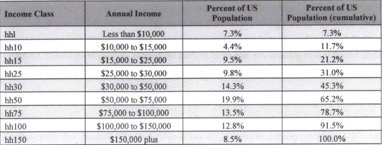
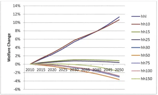
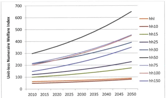
Like USREP, there are nine household income classes in the model used for this study, as displayed in Table I below. In addition to displaying the household income levels for each category, Table 1, shows the percentage of the total US population (in 2006) that fits within each category. For every state, the number of households per income group and overall population are estimated using data from the US Census (2009) through 2030. Beyond 2030, population growth rates in each state are applied uniformly across all income groups. How households earn income and the goods on which this income is spent varies by state. Household savings are an integral part of the consumer utility function, which makes the "consumption-investment decision endogenous" (Rausch et al 2010). The model employs an approach laid out by Bovenberg, Goulder and Gurney (2005), where household capital invested in the production of market goods and services is separated from capital that is invested back into the household (residential capital). The model assumes that income from the former is subject to taxation, while the later is not, and the model affords households the flexibility to shift their investments accordingly.

Table 1. Model Income Classes and Population $10,000 to $15,000 hhl5 $15,000 to $25,000 9.5% 21.2% hh25 $25,000 to $30,000 9.8% 31.0% hh3O $30,000 to $50,000 14.3% 45.3% hh50 $50,000 to $75,000 19.9% 65.2% hh75 $75,00 to $100,000 13.5% 78.7% hh100 $100,000 to $150,000 12.8% 91.5% hh150 $150,000 plus 8.5% 100.0%

Finally, tax rates are differentiated by region and industry sector, and include both federal and state tax regimes. Tax revenues for each state are distributed proportional to current levels. Varying state tax levels and the current distribution of Federal tax revenue among the states is incorporated within these

assumptions. The "intent here [is] to keep a focus on the implications of CO2 pricing and revenue distribution, and not muddy that by assuming changes in distribution of other Federal or State tax revenues" (Rausch et al 2009). The model includes ad-valorem, income and payroll taxes, with rates set

according to a combination of IMPLAN data on inter-institutional taxation and NBER TAXSIM data on marginal personal income tax rates. (Rausch et al 2009).

4. Policy Framework for Analysis: The CLEAR Act

This paper explores the broader question of the economic consequences of a nation-wide limit on greenhouse gas emissions by applying the model described above to the Carbon Limits and Energy for America's Renewal (CLEAR) Act, a federal bill introduced in 2009 by Senators Maria Cantwell (D-WA) and Susan Collins (R-ME). CLEAR was proposed as an alternative to the most recent generation of cap-and-trade policies, the American Clean Energy and Security (ACES) Act (otherwise known as Waxman-Markey) (H.R. 2454) and the American Power Act (S. 1733). Both of these bills focused on a cap-and-trade program where permits would be freely allocated in early years, and where a large percentage of emissions reductions would come from international offset projects. While ACES passed the House, the overall legislative effort failed in the Senate, in no small part due to concern about the economic costs of pricing carbon and state-level distribution questions. This concern came primarily from conservative elected officials and think tanks, yet also from Democratic officials from carbon or energy intensive states like Senator Joe Manchin of West Virginia, who aired an infamous campaign ad of himself firing a rifle round through a copy of "The Cap And Trade Bill," proclaiming that "it's not good for West Virginia."

Many environmentalists also opposed the ACES/APA combo, arguing that its permit giveaways and heavy reliance on offsets begged for regulatory evasion and gaming, ultimately risking the ability to adequately control greenhouse gases. The CLEAR Act responded to these manifold concerns, by requiring all permits to be auctioned, minimizing international offsets, and by recycling revenues (as explained below) in a progressive way that could produce net benefits for many households. CLEAR continues to be discussed on Capitol Hill with plans for re-introduction in the 11 3k" Congress in 2013.

CLEAR utilizes a "cap-and-dividend" approach, which begins with a quantitative limit (a "cap") on fossil carbon emissions, not unlike cap-and-trade. The cap is implemented through the issuance of a limited number of CO2 emissions permits, which are auctioned monthly by the US Treasury and where each ton

of carbon dioxide introduced into the US economy must be covered by a permit. The annual number of permits declines over the lifetime of the policy, making the cap increasingly stringent.4 CLEAR's cap addresses CO2 only, although non-binding provisions for reducing other greenhouse gases are included in

the bill as well.

The CLEAR Act proposes to auction 100% of emission permits. These auctions are estimated to generate hundreds of billions of dollars annually-a significant new revenue source for the federal government. How these revenues are used, of course, greatly determines the overall economic efficiency as well as the incidence of the policy. As will be discussed in great detail below and as is touched on above, the incidence inquiry is concerned with the question of who in society will bear the economic burden of a given policy. Of special concern is whether a policy is progressive or regressive, as discussed above. CLEAR uniquely allocates the lion's share (75 percent) of revenues to US citizens, through the form of an annual flat-rate rebate. This rebate is what is referred to as the "dividend" in the "cap-and-dividend" framework. The fact that the rebate is flat-meaning it is the same amount of money for all US citizens, regardless of their income level-makes the policy powerfully progressive, for a given sum (say $1,000) is of much greater marginal value for low-income households (in proportion to their annual income) than it is for middle- and upper-income households.

The remaining 25 percent of revenues from CLEAR Act permit auctions are allocated to a fund called the Clean Energy Reinvestment Trust (CERT) Fund. The CERT Fund is designed to provide capital for a range of programs and incentives that either drive down emissions further or help address unwanted policy impacts. For example, the CERT Fund would provide "targeted and region-specific transition assistance to workers, communities, industries and small businesses of the United States experiencing the

greatest economic dislocations," (CLEAR Act legislative text) including training programs for the new clean energy economy, compensation for the early retirement of carbon intensive facilities and assistance to energy-intensive industries facing international competition not subject to a carbon price. The Fund would also pay for adaptation efforts, clean energy and energy efficiency projects, projects that reduce greenhouse gases other than C0 2, and programs that provide special support for low-income families struggling with energy costs. The CERT Fund has the capacity to drive down emissions beyond what the cap alone would accomplish; alternately, the CERT Fund could reduce compliance costs, by offering financial support to companies transitioning away from fossil fuels towards clean energy. The many benefits of the CERT Fund are not included in the modeling exercise that follows, nor are other of the bill's components such as the Voluntary Carbon Reduction program, Manufacturing Innovation Credits, Supplemental Emission Reduction Credits, or the Regional Dividend Adjustment clause. This means that the estimated costs of the CLEAR Act will be slightly inflated in what follows. In addition, this means that the discrepancies between states will also be overestimated, because many of the programs under the CERT Fund are aimed at smoothing geographical disparities, in addition to the Regional Dividend Adjustment program. I do not claim to have represented the economics of the CLEAR Act in its entirety

in this study. Rather, CLEAR provides a jumping-off point to investigate some of the dominant issues and trends in the US climate policy debate more generally.

5. Model Results

This section presents results from the CGE model described in Section 3, simulating the economic and environmental performance of the CLEAR Act. CLEAR has been selected to investigate the possible economic dynamics of a US climate policy more broadly. Section 5 begins by outlining three CLEAR Act scenarios being considered by Cantwell staff. I first analyze the CO2 emissions reductions under each

scenario, estimating annual as well as cumulative reductions. Second, I look at the aggregate national welfare impacts due to the implementation of the first scenario only. Third, I investigate distributional questions at the household level, presenting national averages by income class. Section 5 concludes with results on the distributional effects across the 50 United States, providing new perspectives on the political economy of US climate policy.

5.1 Policy Scenarios

The first of the three policy scenarios represents the emissions reduction pathway specified in the CLEAR Act, as introduced in 2009. The second and third scenarios are being considered by the Cantwell office to temper the overall economic impact of the Act and to allow for adaptation of the requirements beginning in 2030. These modifications are inspired by the recognition that, in 2030, decision makers should have

more information about abatement costs and the pace and severity of climate change; and that this new information will allow them to make adjustments to optimize the policy. All three scenarios assume that implementation would begin in 2015, later than originally considered in the CLEAR Act.

All three scenarios are compared with a Reference case, which should be seen as the "business-as-usual" pathway-the world without climate policy-from 2006 to 2050. As explained in detail in Section 3, the Reference case is based upon 2006 economic data provided by 1MPLAN and TAXSIM, as well as primary energy consumption estimates and electricity generation mix profiles from the US Energy

Information Administration's (EIA) State Energy Data System (SEDS). These data are extrapolated into the future by the recursive dynamic component of the model using assumptions about growth rates for

metrics such as population and productivity, along with resource depletion curves for raw fossil fuel reserves and declining cost curves for emerging technologies such as wind, solar and geothermal. Such assumptions in turn shape growth in investment and GDP. US GDP in the Reference case grows at an average compound annual growth rate of 2 percent per year from 2006 to 2050, and most states see similar rates. CO2 emissions, under the Reference case, grow at an average compound annual growth rate of 1 percent, from 5,874 million metric tons (MMT) in 2006 to 9,210 MMT in 2050, an overall growth of 57 percent. During the period between 2006 and 2010, CO2 emissions decline due to the beginning of the

recession. By 2015, the model assumes the nation is returning to an increasing quantity of emissions from the 2010 nadir. It is important to note that the model does not include the latest natural gas price

projections due to hydraulic fracturing, nor does it incorporate assumptions related to the recent US EPA emissions regulations on greenhouse gases and mercury (and how these will affect the economics of any new or expanded coal fired power plants). Figure 1, Figure 2, Figure 3 and Figure 4 below all show the Reference case plotted alongside the various policy cases.

Scenario 1 (Si)

As stated above, Scenario I follows the emissions reduction pathway laid out in the introduced version of the CLEAR Act, modified by the assumption that the policy would be reintroduced in 2013. CLEAR stipulates a two-year window between its enactment and the first year of emissions regulation. This means that emissions would begin to be capped in 2015, however the number of allowances issued for that year would be set according to estimates of 2015 business-as-usual emissions levels to ease industry into the regime. The amount of allowances issued in 2015 is then held constant for two more years (through 2017). After 2017, the number of allowances is reduced by 0.25 percent per year, creating an increasingly strict cap and reducing CO2emissions nationwide.

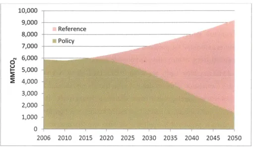
10,000 9,000 8,000 Reference 8,000 aPohicy 7,000 6,000 0 5,000 -2 4,000 3,000 2,000 1,000 0 2006 2010 2015 2020 2025 2030 2035 2040 2045 2050

Figure 1. Scenario 1 CO2 Emissions Trends (MMT)

Figure 1 above depicts the downward-sloping trend in emissions due to the increasingly restrictive cap ("Policy"). This trend is superimposed on the upward-sloping growth in emissions projected under the "business-as-usual" Reference case ("Reference"). In 2015, the estimated quantity of US CO2 emissions

is 5,964 million metric tons (MMT), which is the number of permits issued for that year (5,964 million permits, at one permit per metric ton). In 2020, the Reference case projects the US to emit 6,257 MMT CO2, whereas the number of permits issued by the US Treasury in that year is cut to 5,875 million (at one permit per metric ton), a reduction of 382 MMT. This trend continues: in 2030, the Reference case estimate is 7,037 MMT CO2, while only 4,738 million permits are auctioned, yielding a reduction of 2,299 MMT; in 2040, the Reference case projects 8,028 MMT CO2 compared to 2,950 million permits, a cut of 5,078 MMT; and in 2050, the spread is between 9,210 MMT (Reference) and 1,408 million available permits, a difference of 7,802 MMT CO2. The emissions reduction trajectory presented by Scenario 1 achieves the following annual CO2 reductions relative to the 2006 baseline: 19 percent

reduction by 2030, 50 percent by 2040 and 76 percent by 2050, as indicated below in Table 2.

Cumulatively, Scenario 1 cuts emissions levels (from 2015-2050) to 147 billion metric tons (BMT) CO2, relative to the Reference level of 266 BMT C02, producing nearly a 45% reduction in cumulative

emissions over the 35 year period.

The emissions reduction pathway shown in Figure 1 portrays the exact emission quotas represented in the CLEAR cap, in five-year increments. The actual emissions reduction pathway may look more like Figure 2, where the effects of "banking" and "borrowing" smooth the downward slope of emissions abatement,

while also smoothing the upward slope of CO2 emissions permit prices (as explained in greater detail

below). Banking is a provision that allows regulated companies to purchase emissions permits in advance, to be set aside for future use, akin to money secured in a bank. Borrowing is the opposite provision, which allows companies to forestall the purchase of permits, assuming future liabilities. These nuances improve the economic efficiency of the policy, and provide financial flexibility to regulated firms (Bosetti, Carraro and Massetti 2009; Leiby and Rubin 2001). The CLEAR Act includes both banking and borrowing. Within this formulation of the model, however, there is zero demand for borrowing, while banking plays a crucial role in reducing policy costs. Therefore, the remainder of this paper refers to banking only. Scenario 1 under the assumption of unlimited banking will here forward be referred to as Scenario 1b, and the same notation will be applied to the other two scenarios as well.

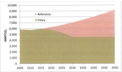
Figure 2 projects Scenario lb-Scenario 1 under the assumption of unlimited banking. Unlimited banking here refers to a policy provision where there is no restriction on the amount of time that a banked permit can be held before being surrendered to the US Treasury to fulfill an emissions liability. Unlimited banking as represented in this model, however, does include two important constraints on the amount of banking. First, the percentage of banking allowed (relative to the CO2 permit quota stipulated for a given

year in the CLEAR Act) is constrained to 15 percent in the first year of the policy (2015) and to 20 percent for every year thereafter. For example, in 2015 the emissions cap is 5,964 million metric tons, therefore the maximum number of bankable permits is 895 million (15 percent of 5,964 million, at one permit per ton). The second constraint is that the compound annual growth rate at which the price of CO2

emission permits rise cannot be less than 5 percent. The first constraint is based on feasibility thresholds stipulated by Cantwell legislative staff, and informal modeling of the CLEAR Act conducted by the US EPA. The second constraint is based on the assumption that no firm would invest in a financial instrument (CO2 permit) that is rising at a rate less than the rate of interest (which has been assumed to be

approximately 5 percent for the life of the policy). Welfare costs can be driven lower than those indicated below in the unlimited banking case if either of these constraints are relaxed.

10,000 - - -- -- - -9,000 Reference 8,000 M Poh0cy 7,000 6,000 5,000 1,0005 0 2006 2010 2015 2020 2025 2030 2035 2040 2045 2050

Figure 2. Scenario lb CO2 Emissions Trends (MMT) - Unlimited Banking

Scenario 2 (S2)

Scenario 2 takes a slightly less aggressive approach overall. It is nearly identical to Si until 2030, at which point the rate of declination in CO2 allowances remains constant at 3.5 percent (the result of

declining at 0.25 percent for 13 years (2018 through 2030)), instead of continuing to decrease 0.25 percent per year as in SL. One minor additional difference is that S2 begins to decrease the number of emissions allowances in 2016 rather than 2017. Therefore, under both Si and S2 the same number of permits are issued in 2015, however for every year thereafter they are slightly different. In 2020, the amount of permits under SI is 5,875 million while under S2 there are 5,816 million. In 2030, there are 4,738 million permits under Si and 4,572 million under S2; and by 2050 there are 1,408 million permits under Si and 2,242 million under S2. Scenario 2 is slightly more aggressive than Si up to 2030 (due to an earlier start in the 0.25 percent per year allowance quantity reductions), however Si ultimately achieves deeper emissions reductions. For example, the S2 emissions reduction pathway (displayed in Figure 3) achieves the following annual CO2 reductions relative to the 2006 baseline: 22 percent reduction by 2030, 45 percent by 2040 and 62 percent by 2050, as indicated below in Table 2. Cumulatively (from 2015-2050), Scenario 2 achieves emissions levels of 151 BMT C02, producing nearly a 43% reduction from Reference case levels-only 2% less than Scenario 1.

10,000 - -- - -9,000 0 Reference 8,000 C 7,000 - - - -

-6

Figure 3. Scenario 2 CO2 Emissions Trends (MMT)

Scenario 3 (S3)

Scenario 3 is the least aggressive approach, and leaves a great deal of discretion open to future decision makers. S3 follows the pathway of S2 until 2030, at which point the cap remains flat for the duration of the policy.5 Figure 4 below shows the emissions reduction pathway for S3. From 2015 through 2030, emissions levels reflect the number of permits issued (which is the same under S2 and S3). In 2030, the number of permits is 4,572 million. Under S3, this is the amount of permits issued in every subsequent year, indicated by the flat "Policy" slope in Figure 4. This is in contrast to S2 where from 2030 on the number of permits continues to decline at the constant rate of 3.25 percent per year. Under Scenario 3, the maximum annual emissions reduction from the 2006 baseline is 22 percent, first achieved in 2030 (see Table 2 below). Cumulatively, Scenario 3 reduces 35-year emissions levels (from 2015-2050) to 151 BMT CO2, producing a 32% reduction from Reference case levels.

5 Again, as explained above, the notion here is that decision makers would have to reassess appropriate emissions

10,000 - - - - -_ -9,000 mReference 8,000 7,000 -4,000 2,000 W 1,000 0 2006 2010 2015 2020 2025 2030 2035 2040 2045 2050

Figure 4. Scenario 3 CO2 Emissions Trends (MMT)

Table 2. Annual CO2 Emissions Levels Relative to 2006

S.2

Background on Welfare Analysis

The most basic economic outcome of the CLEAR Act is the establishment of a price on carbon. This internalizes the environmental damages associated with unabated emissions and drives up the cost of carbon intensive energy, such as coal and petroleum products, which most Americans depend on to power their modern lifestyle.6 Recent developments in the extraction of natural gas may temper this increase in consumer energy prices, for gas is less carbon intensive than coal and increasingly less costly regardless of the price on carbon. Nonetheless, natural gas itself will have to be phased-out due to its fossil carbon content likely starting in the mid-to-late 2020s and early 2030s (as indicated by model results). Many renewable energy sources such as wind and solar are also rapidly declining in cost, however due to constraints such as intermittency it is likely that a carbon-free energy provision system (generation, storage, grid and all) will be more expensive than the current system which is based on fossil energy. Therefore, an increase in the price of energy is likely under the CLEAR Act.

6

Coal

As the price of energy rises, overall consumption rates will tend to decline throughout the economy. This downward trend in consumption is the result of a reduction in buying power, which effectively represents a drop in the value of household income. Using the framework established by Rausch et al (2010), consumption (1), leisure (2) and residential capital (3) represent the full value of household income in this model, and full income is the primary indicator of welfare.! Therefore, a percentage change in full income (measured as equivalent variation) from the Reference case indicates the change in welfare due to policy

implementation. One can understand these welfare changes as the basic economic cost of the policy.

Under the CLEAR Act, household welfare costs are partially or entirely (depending on income class) offset by an increase in household income through the dividends produced by the policy (described

above). There is therefore a tension between the beneficial affect of the dividend mechanism and the detrimental impact of increased costs of energy associated with the cap mechanism. These two are opposing forces in an economic tug-of-war, the result of which determines a given household's or a given state's change welfare (either positive or negative) due to the implementation of the policy.

Finally, when considering changes in welfare in the context of climate policy it would be incomplete to ignore the many welfare benefits of mitigating environmental damage-these benefits are, after all, the fundamental impetus for a policy to reduce greenhouse gas emissions. A special class of models called integrated assessment models8 (IAMs) has offered an initial response to this problem by producing a metric called the social cost of carbon (SCC). The social cost of carbon estimates the "monetized damages associated with an in incremental increase in carbon emissions" (Greenstone et al 2011). This estimate includes (but is not limited to) "changes in net agricultural productivity, human health, property damages from increased flood risk, and the value of ecosystem services" (Greenstone et al 2011). By incorporating this metric into a cost-benefit analysis, every ton of CO2 reduced has a tangible economic

benefit to society and therefore improves welfare, further offsetting the costs of a policy like the CLEAR Act. While it is arguably impossible to establish a metric that perfectly reflects the many benefits of something as complex as an Earth with reduced anthropogenic climate forcing, it is arguably a step forward to approximate such benefits, such that a more thorough accounting can take place in academic

7 There are many other dimensions to welfare, such as public health issues associated with the social cost of carbon.

These factors are not included in this study, however it is recommended that future modeling efforts do aim to incorporate them.

8 Integrated assessment models "integrate" scientific data from Earth systems, such as the atmosphere, the oceans, terrestrial ecosystems, etc. with data on the human economic system. Examples of prominent IAMs include the MIT EPPA (Emission Prediction and Policy Analysis) model, the DICE (Dynamic Integrated Climate and Economy) model, developed by economist William Nordhaus, the PAGE (Policy Analysis of the Greenhouse Effect) model produced by Chris Hope, and the FUND (Climate Framework for Uncertainty, Negotiation and Distribution) model developed by economist Richard Tol.

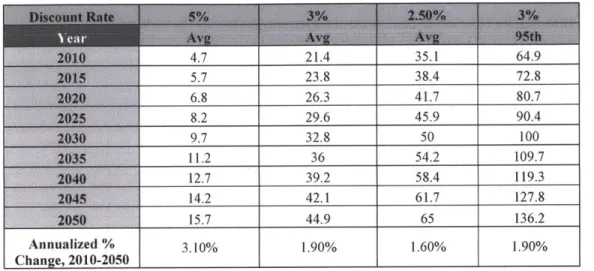
and decision-making forums. Indeed, an interagency working group in the United States government established SCC values in 2010 to be applied to regulatory analyses (Greenstone et al 2011), as presented in Table 3 below.

Table 3: Social Cost of CO2 (short ton), 2010 - 2050 (2007 dollars)

9 21.4 35.1 64.9 5.7 23.8 38.4 72.8 20" 6.8 26.3 41.7 80.7 2 8.2 29.6 45.9 90.4 9.7 32.8 50 100 11.2 36 54.2 109.7 12.7 39.2 58.4 119.3 14.2 42.1 61.7 127.8 2050 15.7 44.9 65 136.2 Annualized % 3.10% 1.90% 1.60% 1.90% 1Change, 2010-20501 111

Unfortunately, incorporation of the social cost of carbon into the CGE model used for this study was not possible. Nonetheless, to provide an initial estimate of how the SCC may affect model results, I have

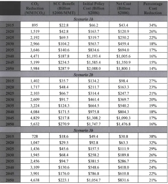
done a post-hoc "back of the envelope" calculation. The calculation is a simple multiplication of the social cost of carbon values listed under the 3 percent (median) discount rate above by the amount of carbon reduced under each of the three scenarios. Table 4 below presents the various results for all three scenarios, under the assumption of unlimited banking.

The first column of Table 4 presents the CO2 reductions associated with each policy, again assuming

unlimited banking, which shifts emissions reductions forward in time (firms choose to reduce emissions more aggressively due to the benefits of banking, as discussed above). The emissions reduction figures in Table 4 are in the unit million metric tons (MMT). The social cost of carbon estimates presented in Table 3 have therefore been converted to metric tons from short tons (the unit of measure in Table 3).

Additionally, the figures from Table 3 have been converted from USD 2007 to USD 2006, which is the unit used throughout this paper. The second column in Table 4 is the product of the total amount of CO2

reduced for a given scenario and year and the social cost of carbon estimate. This is seen as the benefit of the policy, for it is averted social costs associated with reduced carbon emissions. The third column portrays the initial economic cost of the policy (not including the SCC benefits), which is the difference

9 Source: Greenstone et al (2010), Table 4.

between US GNP estimates in the Reference case and under the given scenario. The fourth column in Table 4 is the net of the initial policy costs and the benefits associated with reducing carbon as measured by the SCC. The final column portrays the percentage by which the incorporation of the social cost of carbon reduces the aggregate (national) policy costs.

Table 4. Back of the Envelope Estimate of the Benefits Associated with Reducing CO2,

per Social Cost of Carbon (SCC) Estimates (Assuming a 3 Percent Discount Rate)

895 $22.8 $66.2 $43.4 34% 1,519 $42.8 $163.7 $120.9 26% 2,192 $69.5 $319.7 $250.2 22% 2,966 $104.2 $563.7 $459.4 18% 3,646 $140.6 $834.6 $694.0 17% 4,471 $187.8 $1,193.4 $1,005.6 16% 5,199 $234.5 $1,585.4 $1,350.9 15% 5,984 $287.9 $2,088.0 $1,800.1 14% 1,402 $35.7 $134.2 $98.4 27% 1,717 $48.4 $211.7 $163.3 23% 2,103 $66.7 $314.4 $247.7 21% 2,609 $91.7 $461.4 $369.7 20% 3,224 $124.3 $664.5 $540.2 19% 4,084 $171.5 $975.8 $804.3 18% 4,829 $217.8 $1,308.2 $1,090.3 17% 5,632 $270.9 $1,747.7 $1,476.8 16% 728 $18.6 $49.4 $30.8 38% 1,047 $29.5 $92.8 $63.3 32% 1,436 $45.6 $157.5 $111.9 29% 1,945 $68.4 $258.2 $189.8 26% 2,456 $94.7 $381.5 $286.7 25% 3,109 $130.6 $548.6 $418.0 24% 3,901 $176.0 $786.8 $610.8 22% 4,638 $223.1 $1,054.7 $831.6 21%

The social cost of carbon does not wholly offset the economic costs of the policy under any of the three scenarios, and the percentage cost reduction declines over time under each scenario as the economic costs of the policy outpace benefits from reducing carbon. The reader should consume this information with caution. A full accounting of the benefits associated with the social cost of carbon requires a more thorough integration within the model, and it is likely that the benefits are under-estimated in Table 4. This is a rough approximation that provides a starting point for understanding the economic benefits of

reducing carbon emissions.

While the estimates above indicate that the social cost of carbon does not fully nullify policy costs, it is clear that the SCC does reduce policy costs. Therefore, all welfare changes presented below are skewed more negatively than they would be were the SCC included. Future efforts should aim to integrate the SCC to produce a comprehensive picture of welfare changes.

5.3 Aggregate Welfare Impacts

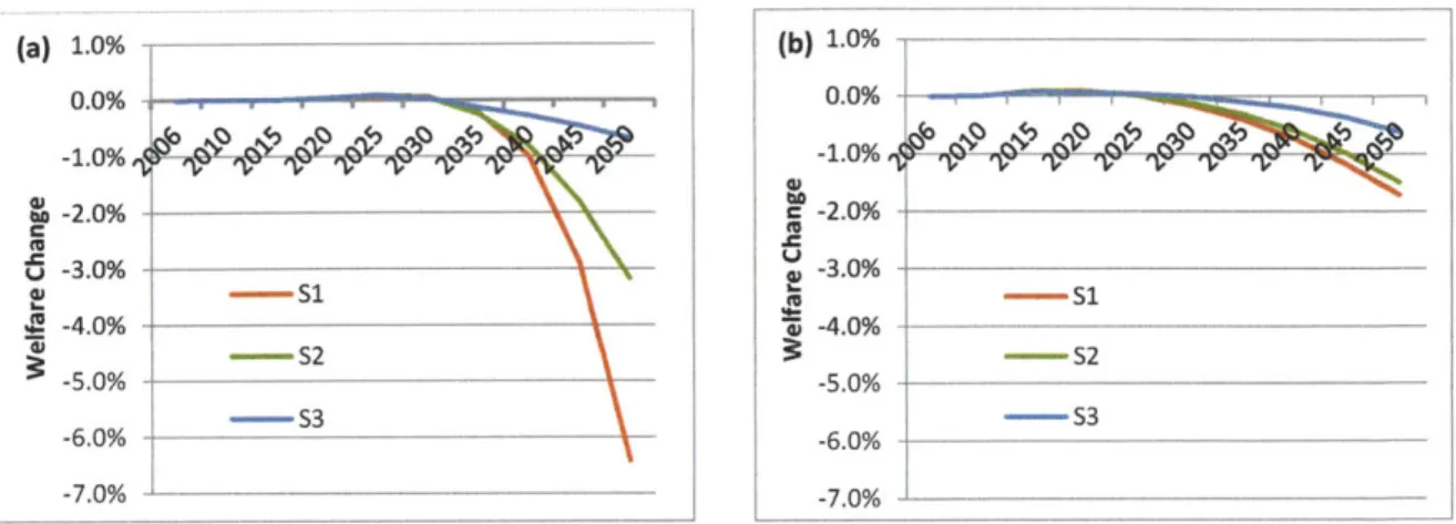
Figure 5 below depicts the average welfare changes of each of the three policy scenarios, under assumptions of both (a) no banking and (b) unlimited banking. Welfare change is calculated as the difference in income between the Reference case and the given policy scenario, divided by the original Reference case income level. Scenario 1b, which produces the greatest emissions reductions, generates a decline in average household welfare of 0.2 percent in 2030, 0.7 percent in 2040 and 1.7 percent (from the Reference case) in 2050. Scenario 2b is only slightly different from S1, with welfare reductions of 0.1 percent in 2030, 0.6 percent in 2040 and 1.5 percent in 2050. Finally, Scenario 3b, which produces the smallest emissions cuts, reduces welfare by 0 percent in 2030, 0.2 percent in 2040 and 0.6 percent in 2050. All scenarios show the beneficial impact of banking, and escalating policy costs over time (reflected in a greater percentage decrease in welfare). Additionally, under unlimited banking, the difference in welfare costs between S1, S2 and S3 is much smaller than under no banking.

(b) 1.0% 0.0% -1.0% -2.0% -3.0% -4.0% -5.0% - -S3 -6.0% -7.0%

-Figure 5. Welfare Changes Due to Implementation of the CLEAR Act

The welfare changes depicted above are largely a function of CO2 emissions allowance values, or permit prices, and their propagation throughout the economy. Figure 6 below shows the radical increase in allowance values over time when banking is not permitted, and Figure 7 shows the "price-smoothing" affect of unlimited banking. It is also important to note that the CLEAR Act includes a "price collar" or a "symmetric safety valve" (Burtraw et al 2010), which protects the market from excessively high or low price shocks by stipulating both a "price floor" (minimum price) and a "price ceiling" (maximum price).

$400.00 - - --- - -$350.00 --- ~---CLEAR Ceiling--- $300.00 -- - CLEAR Floor --

51

Figure 6. CO2 Emission Allowance Values - No Banking

The existence of a price collar, however, does not negate the need for other policy measures (such as banking) that have the above-mentioned price smoothing affect (Jacoby and Ellerman 2004). For

(a) 1.0% 0.0% -1.0% o -2.0% 6 -3.0% -Si 4 -4.0% 4' -5.0% _- 2 --- S3 -6.0% -7.0%