Deploying fast object detection for micro aerial vehicles

Deploying Fast Object Detection for Micro Aerial

Vehicles

by

Nicholas Florentino Villanueva

Submitted to the Department of Aeronautics and Astronautics

in partial fulfillment of the requirements for the degree of

Master of Science in Aerospace Engineering

at the

MASSACHUSETTS INSTITUTE OF TECHNOLOGY

June 2018

@

Massachusetts Institute of Technology 2018. All rights reserved.

Signature redacted

A u th o r ...

...

Department of Aeronautics and Astronautics

May 24, 2018

Certified by...

Accepted by...

MASSACHUSETTS INSTITUTE OF TECHNOLOGY

JUN 2.8 2018

LIBRARIES

Signature redacted

Nicholas Roy

Professor of Aeronautics and Astronautics

Thesis Supervisor

Signature redacted

...

Hamsa Balakrishnan

Associate Professor of Aeronautics and Astronautics

Chair, Graduate Program Committee

Deploying Fast Object Detection for Micro Aerial Vehicles

by

Nicholas Florentino Villanueva

Submitted to the Department of Aeronautics and Astronautics on May 24, 2018, in partial fulfillment of the

requirements for the degree of

Master of Science in Aerospace Engineering

Abstract

In this thesis, we present an evaluation of four state of the art convolutional neural network (CNN) object detectors, and a method to incorporate temporal informa-tion into an object detecinforma-tion pipeline for a micro aerial vehicle (MAV). This work was done as part of the Defense Advanced Research Projects Agency's (DARPA) Fast Lightweight Autonomy (FLA) program with the goal of creating an autonomous MAV that could explore and map an unknown urban environment. We tested four CNN-based object detectors on a range of compact deployable compute devices in or-der to select the best detector-hardware pair for our flight vehicle. We chose to use the MobileNetSSD object detector running on an Intel NUC Skull Canyon. Additionally, we developed an efficient object detection method that incorporates temporal infor-mation found in sequential camera frames by selectively utilizing an object tracker when the object detector fails. Our temporal object detection method shows promis-ing results improvpromis-ing the recall of the base object detector on two of three datasets while maintaining a high framerate.

Thesis Supervisor: Nicholas Roy

Acknowledgments

I would like to thank my advisor, Nicholas Roy, Professor of Aeronautics and Astro-nautics at MIT. Nick has been my advisor at MIT through both my undergraduate and graduate careers and has been a great mentor to me both academically and through his leadership. I would also like to thank Jake Ware, John Carter, the FLA team, and the Robust Robotics Group for their support, without which this wouldn't have been possible.

Additionally, I would like to thank the Lemelson Foundation for their assistance this year.

Lastly, to my friends and family who were with me for all the good times and the bad, thank you for sticking with me.

Contents

1 Introduction

1.1 The Problem .... ...

1.2 Our Approach . . . . 1.2.1 Neural Network Object Detector Evaluation 1.2.2 Object Detection for Micro Aerial Vehicles 1.2.3 Contributions . . . . 1.2.4 Thesis Outline. . . . .

2 Background

2.1 Convolutional Neural Networks . . . . 2.2 Object Detection . . . . 2.3 Object Detection Evaluation . . . . 2.4 Object Tracking . . . . 2.5 Object Detection in Video . . . .

3 Convolutional Neural Network Object Detector 3.1 You Only Look Once v2 (YOLOv2) ...

3.2 Tiny YOLO ...

3.3 The Single Shot MultiBox Detector (SSD) ....

3.3.1 MobileNetSSD ... 3.4 Test Setup ...

3.5 NVIDIA TitanX GPU and Intel Core i7-6700K CPU 3.6 NVIDIA Jetson TX1 Network Evaluation ...

Evaluation Network Evaluation . . . . 15 15 19 19 20 21 21 23 23 26 29 31 33 37 39 42 43 46 48 49 52

3.7 NVIDIA Jetson TX2 Network Evaluation ... 3.8 Intel Movidius Neural Compute Stick Network 3.9 Intel NUC Skull Canyon Network Evaluation . 3.10 Testing Results . . . .

4 Object Detection Flight Vehicle Deployment 4.1 Training MobileNetSSD . . . .

4.1.1 Dataset: OpenImages . . . . 4.1.2 Training Setup . . . . 4.2 Vehicle Integration . . . .

Evaluation

5 Towards Temporally Consistent Object Detection 5.1 Object States . . . . 5.2 Similarity Metric . . . . 5.2.1 Object Color . . . . 5.2.2 Intersection Over Union (IOU) . . . . 5.2.3 Bounding Box Dimensions . . . . 5.2.4 Bounding Box Size . . . . 5.3 Pipeline Overview . . . . 5.3.1 Find Dropped Objects . . . . 5.3.2 Find Close Detections . . . . 5.3.3 Determine In-Frame . . . . 5.3.4 Object Recovered . . . . 5.3.5 Object Tracking . . . . 5.4 R esults . . . . 5.4.1 Camp Lejeune . . . . 5.4.2 Medfield State Hospital . . . . 5.4.3 Guardian Center . . . . 5.4.4 Discussion . . . . 54 58 59 62 65 66 67 68 69 71 72 74 74 75 75 76 77 78 78 78 79 80 81 82 86 90 93

6 Conclusion 97

6.1 Summary ... ... 97

6.2 Contributions . . . . 98 6.3 Future W ork . . . . 99

List of Figures

1-1 An example of an object detection . . . .

2-1 A fully connected three layer neural network. . .

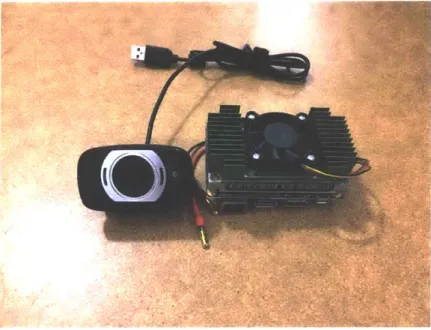
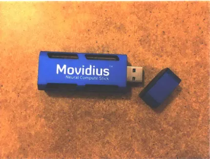
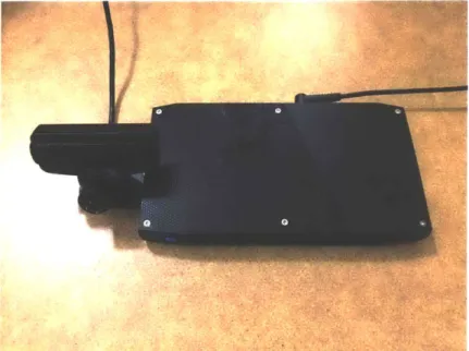
Intersection over union . . . . Anchor boxes over a feature map . . . . Depthwise separable convolution . . . . NVIDIA Jetson TX1 . . . . NVIDIA Jetson TX2 with Connect Tech Orbitty Carrier Board Intel Movidius Neural Compute Stick . . . . Intel NUC Skull Canyon setup with Play Station Eye Camera.

4-1 FLA Quad ...

4-2 Annotated image . . . .

Temporally inconsistent detections . . . . O bject States . . . . Overlapping low confidence detections . . . . Cam p Lejeune . . . . Camp Lejeune TOD results for people . . . . Camp Lejeune TOD results for cars . . . .

TOD detections compared to baseline detections . . . .

TOD poor detection result . . . . Average framerate of TOD vs the baseline on the Camp Medfield TOD results for people . . . .

. . . . 66 . . . . 67 . . . . 72 . . . . 73 . . . . 79 . . . . 83 . . . . 84 . . . . 85 . . . . 86 . . . . 87 Lejeune dataset 87 . . . . 88 3-1 3-2 3-3 3-4 3-5 3-6 3-7 . . 17 . . 24 . . 40 . . 41 . . 47 . . 52 55 . . 59 . . 60 5-1 5-2 5-3 5-4 5-5 5-6 5-7 5-8 5-9 5-10

5-11 Medfield TOD results for cars . . . . 89 5-12 TOD detections compared to baseline detections and labeled data 90 5-13 Average framerate of TOD vs the baseline on the Medfield dataset . 91

5-14 Positive and negative results of overlap non-maximum suppression . 92

5-15 Guardian Center TOD results for people . . . . 93 5-16 Guardian Center TOD results for cars . . . . 94 5-17 Average framerate of TOD vs the baseline on the Guardian Center

List of Tables

Object Detector Requirements . . . . Intel Core i7-6700K CPU Specifications . . . . NVIDIA Titan X GPU Specifications . . . . Desktop GPU Network Evaluation Results . . . . . Desktop CPU Network Evaluation Results . . . . . QUAD ARM CPU Specifications . . . . Maxwell GPU Specifications . . . . Jetson TX1 GPU Network Evaluation Results

Jetson TX1 GPU Network Evaluation Results (CPU Jetson TX1 CPU Network Evaluation Results . . . QUAD ARM and Dual Denver CPU Specifications Pascal GPU Specifications . . . . Jetson TX2 GPU Network Evaluation Results . . . Jetson TX2 GPU Network Evaluation Results (CPU Jetson TX2 CPU Network Evaluation Results . . .

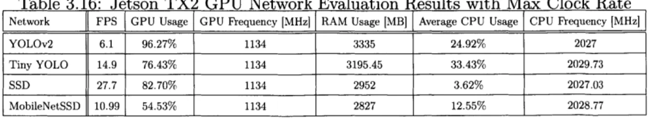
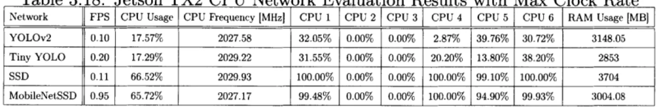
Co 3.1 3.2 3.3 3.4 3.5 3.6 3.7 3.8 3.9 3.10 3.11 3.12 3.13 3.14 3.15 3.16 3.17 3.18 3.19 3.20 3.21 3.22 . . . . 38 . . . . 49 . . . . 49 . . . . 51 . . . . 51 . . . . 52 . . . . 53 . . . . 53 re Usage) . . 54 . . . . 54 . . . . 55 . . . . 55 . . . . 56 e Usage) . . 56 . . . . 56 Jetson TX2 GPU Network Evaluation Results with Max Clock Rate . Jetson TX2 GPU Network Evaluation Results (CPU Core Usage) with M ax Clock Rate . . . . Jetson TX2 CPU Network Evaluation Results with Max Clock Rate Intel Movidius Neural Compute Stick Network Evaluation Results . Intel Core i7-6770HQ Quad Core CPU Specifications . . . . Iris Pro Graphics 580 Specifications . . . . Intel NUC Skull Canyon GPU Network Evaluation Results . . . .

56 57 57 59 60 60 61 Cor

3.23 Intel NUC Skull Canyon CPU Network Evaluation Results . . . . 61

3.24 Network VOC07+12 Accuracy [mAPI . . . . 63

4.1 OpenImages Downsampled Dataset and Class Distribution . . . . 68

Chapter 1

Introduction

1.1

The Problem

Robots are becoming an ever larger part of our daily lives. Their applications are becoming broader as hardware gets smaller and more powerful and algorithms be-come more effective and efficient. However, in order for robots and humans to work together, machines must have an understanding of the world similar to that of their human counterparts. The necessity for a common understanding highlights the im-portance of semantics for robots, or meaningful labels assigned to the perceived en-vironment. For example, it is important for a home assistant robot to know that an apple is different from a plate when a human asks for a snack. Furthermore, the robot must be able to recognize both the apple and the plate in order to connect their meanings with the immediate environment. This requires a semantic perception sys-tem for the classification of objects. We propose such a semantic perception syssys-tem, specifically, an object detection pipeline, to be used by deployed robots to recognize objects in their environments.

This object detection pipeline was used as part of a larger program called Fast Lightweight Autonomy (FLA) put on by the Defense Advanced Research Projects Agency (DARPA). In the first phase of the program, the goal was to use a micro aerial vehicle (MAV) to locate an item (a red barrel) at the end of a trajectory and return to the start, moving as fast as possible (20m/s) while dodging obstacles. This

environment could range from an outdoor field, to a forest, or to the inside of a warehouse.

In the second phase of the program, the challenge was to explore an urban envi-ronment and create a semantic map of the objects that the flight vehicle encountered during its exploration. To complete this mission, the flight vehicle would need state estimation, depth estimation, local mapping, flight control, behavior selection, object detection, and object localization. The goal was to complete these tasks using only monocular camera methods, the motivation being that images contain a rich source of information that is commonly underutilized. The advent of Convolutional Neu-ral Networks (CNNs), along with advances in classical computer vision techniques, have made using a single camera for the tasks stated above much more reliable for flight vehicles. CNNs in particular have made hard coded feature functions for image analysis largely a thing of the past.

Object detection was used to report back what the vehicle encountered on its exploration of the urban environment. The class of objects that the vehicle was to report were predetermined ahead of deployment. For this mission, the objects to detect were mainly people and cars. These objects are typical in urban environments and knowledge of their locations may be of importance for soldiers deployed in an unknown city assessing possible dangers or points of interest.

An object detection is made by placing a bounding box around each object of interest in a given image with an associated semantic label. An example is shown in Figure 1-1. The detections are then sent to a mapper that localizes the object in the global map to be reported back to the user. While seemingly straightforward, the task of object detection comes with a host of challenges. For example, it is easy for humans familiar with cars to pick them out of an image whether the car is big or small, and regardless of the car's orientation. Cars alone come in all kinds of shapes, sizes, and colors. Additionally, when encountered in the real world they can be found in many different orientations. A large part of the difficulty in the object detection task is generalizing. Not only are there many types of cars, they can be encountered in many different situations. Often times, cars in an environment can be occluded or

Figure 1-1: An object detection consists of a bounding box, a semantic label, and a confidence score.

found in cluttered environments and the object detection system would have to be able to pick out the car from the clutter. This problem becomes even more difficult when the object detection system is asked to classify other objects in addition to cars. There are classical computer vision techniques that can perform object detection in many ways whether it be by breaking an object down into parts

117]

or computing hand crafted features [74]. Unfortunately, these methods can be tedious and often times do not perform well in a variety situations.

A CNN, a type of artificial neural network, on the other hand, is able to learn useful feature functions for analyzing images, eliminating the need for handed coded feature functions. CNNs, once trained on enough data, can learn general representations of many classes of objects. This makes them very accurate detectors outperforming methods that preceded them. The ability of CNNs to generalize is why we chose to use CNN-based object detectors for the flight vehicle. Although many existing object detectors exist, such as Faster R-CNN

158],

You Only Look Once v2 (YOLOv2)

157],

and the Single Shot MultiBox Detector (SSD)

142],

there are still challenges for

deployment.

Part of the DARPA FLA program was to put all the autonomy and image pro-cessing stated above onto a single MAV. A main concern when deploying CNN-based methods is their computational load onboard the vehicle, which often has much less

compute power than the environments where the methods were developed. CNNs, while state of the art, use millions of parameters when computing detections from a single image. This can come at a significant cost especially on a vehicle with a small computational budget. Decreasing the size of the CNN could speed up computation, but would come at a cost to accuracy. On top of this, in an autonomous flight system, the detections need to be sent in real-time to the object localizer to be placed in the global map. The challenge then becomes finding a CNN object detection pipeline that can perform well enough in real-time without consuming the entire computation budget of the vehicle. Many state of the art detectors boast short computation times and high accuracy, but do not tackle the issue of deploying these systems on size-, weight-, and power-constrained devices.

Additionally, the state of the art object detectors are made to detect objects on single images. During deployment, the detector will process sequential images in a live video stream. Due to vehicle movement, lighting changes, and viewpoint changes, some objects detected in one camera frame may not be detected in the next. This can cause object detections to be dropped and may provide too few detections to properly localize the object. Specifically for the DARPA challenge, the MAV is flying through an urban environment where objects are generally sparse. In many cases, the vehicle will encounter objects at a distance or in the periphery of the camera frame, which could mean that several detections are required to localize the object.

To address these problems, we present an evaluation of the runtime and resource consumption of some of the fastest state of the art object detectors. This evalua-tion can aid in the selecevalua-tion of a particular method for devices with relatively lower computation throughput. Additionally, we propose a selective tracking-by-detection method that uses temporal object representations to create more consistent object detections over time.

1.2

Our Approach

The following sections will discuss how we selected an appropriate neural network ob-ject detector for our hardware and incorporated temporal information in the detection pipeline to increase object recall and temporally consistent detections.

1.2.1

Neural Network Object Detector Evaluation

The first step involved selecting an object detection method to put on the vehicle using an analysis of the current state of the art in object detection. Our main criteria in this evaluation were speed, accuracy, and computational resource consumption. To this end, we narrowed down the search space of detectors to CNN-based methods because CNNs are the top performing in terms of accuracy and are highly generalizeable given enough training data. Additionally, all of our proposed hardware on which to deploy the object detector had a GPU, which allowed the detector to reduce its inference time.

Using past evaluations as a starting point such as the one done by Huang et al. [28] and the experimental results from the original object detection papers, we narrowed down our search to the You Only Look Once (YOLO) methods (YOLOv2 [57] and Tiny YOLO [54]) and the Single Shot MultiBox Detector method [421. We chose these methods because they were designed to be both fast and accurate.

The object detection methods were evaluated across selected deployable compute devices that could be used on the flight vehicle. When testing the object detection methods on the devices, we were mainly looking at the test time frame rate and GPU, CPU, and memory usage. The methods were first tested on a desktop machine with an NVIDIA TitanX GPU and Intel Core i7-6700K CPU. After initial testing on a machine without size, weight, and power constraints, we tested the methods on a range of deployable hardware. This included a NVIDIA Jetson TX1, a NVIDIA Jetson TX2, an Intel Movidius Neural Compute Stick, and an Intel NUC Skull Canyon.

After the evaluation of these methods on different hardware, we decided to move forward with the Single Shot MultiBox Detector using MobileNet

127]

as its feature

extractor. We will refer to this combination as MobileNetSSD. This setup ran the fastest while still maintaining reasonable accuracy performance.

We used a version of MobileNetSSD [3] implemented with the Caffe deep learning framework [33]. The network runs entirely on the Intel NUC Skull Canyon using an OpenCL version of Caffe [71] so that we could take advantage of the NUC's GPU for inference.

1.2.2

Object Detection for Micro Aerial Vehicles

Although deploying a CNN object detector onboard a MAV works generally well given that it can run in real-time, most state of the art detection methods were made to address the PASCAL Visual Object Classes detection challenge [151, which measures the accuracy of detectors on a test set of still images. However, when detectors are running on a robot, they process sequential camera frames, and also need to deal with varying object poses and possibly blurred images from motion.

To tackle this problem, we leveraged information present across camera frames to augment the object detection pipeline. Specifically, we increased the confidence of detections on objects the robot has seen before by using a similarity metric based on object color, size, location, and bounding box dimensions. This metric was created by using an adaptive weighting scheme for each of the metric components based on the size of the bounding box in a given frame. Since we know the general shape and size of the objects we are detecting and the environment in which we are flying, the bounding box size roughly relates to the distance from which an object is viewed. Based on this size, we can dynamically weight how much the system should rely on color, bounding box shape and size, and location.

We also leveraged an object tracker in the detection pipeline by selectively apply-ing it to find objects that the detector found in a previous frame, but failed to detect in the current frame. The tracker was selectively applied by using the similarity met-ric to to determine if the object was detected or not. In this way, we only applied the tracker to an object that needed to be detected.

the limited computational capacity onboard the vehicle, and the need to maintain a real-time system. The entire pipeline consists of a detection step, a rescoring step, a tracking step, and a non-maximum suppression step. Although the detection pipeline could be setup with any arbitrary single image object detector and image based object detector, we implemented the system with the MobileNetSSD object detector and GOTURN object tracker [24]. Together, the system runs at a minimum of 40 frames per second on the Intel NUC Skull Canyon.

1.2.3

Contributions

Our first contribution is an evaluation of several state of the art CNN-based object de-tection networks tested across a range of deployable compute hardware. The evaluated object detection networks included YOLOv2, Tiny YOLO, SSD, and MobileNetSSD. The hardware for the evaluation included a NVIDIA Jetson TX1, a NVIDIA Jetson TX2, an Intel Movidius Neural Compute Stick, and an Intel NUC Skull Canyon. The test results can help in selecting an appropriate CNN-based detector and compute-device pair.

The second contribution is a proposed method to incorporate temporal informa-tion into an object detecinforma-tion pipeline that is both effective at increasing detector recall and maintaining a high frame rate. This is done by combining an object detector and an object tracker in an efficient framework where the object tracker is only applied when necessary.

1.2.4

Thesis Outline

This thesis is organized into six chapters. Chapter 2 provides a background for CNNs as well as past and current methods for object detection, object detection evaluation, object tracking, and object detection in videos. Chapter 3 gives a summary of the methodology of the evaluated neural network object detectors. It then provides the results of the object detector evaluation across the tested hardware. Chapter 4 de-scribes how the object detector was deployed on the flight vehicle. Lastly, Chapter

5 introduces the temporal object detector and presents results of the method using data collected in three different environments.

Chapter 2

Background

2.1

Convolutional Neural Networks

At the core of the object detector analysis and our temporal object detector, is the use of convolutional neural networks (CNN). CNNs are a type of artificial neural network that take 2D signals as input; this can include things such as an audio signal or an image. Neural networks are useful because they can approximate complex nonlinear functions. Neural networks are made up of a series of units often referred to as neurons stacked into layers. Each neuron consists of a series of weights wi, a bias term b, and an output function. In a network, a neuron takes in inputs xi from other connected neurons. The output of the neuron is the output function applied to the sum of the weights, wi, times the inputs, xi, plus the bias b. If the output function is a linear function, then the sum of the weighted inputs plus the bias is exactly the output. To produce a nonlinear result, a nonlinear function is applied. Common nonlinear output functions used in neural networks include the tanh(x) function shown in Equation 2.1, the rectified linear unit (ReLU) shown in Equation 2.2, and the leaky rectified linear unit shown in Equation 2.3.

ex - e-X

21

f(x) = max(x, 0)

f) max(x, 0) x >= 0 (2.3)

amin(x, 0) x < 0

The nonlinear function can be chosen depending on the desired output of the neuron, for instance if we wanted to have the output bounded between -1 and 1, or to act as a threshold function on some property of the input. The output of a neuron with an applied nonlinear function, taking n inputs xi, with n weights wi, a bias b, and a nonlinear function f(x) is shown in Equation 2.4.

y =f xiwi+b (2.4)

A neural network is then a series of layers of neurons stacked onto one another as shown in Figure 2-1. The network in Figure 2-1 takes in a column vector x and outputs a single value y. The first layer of the network is the input layer, the middle layer is a hidden layer, and the last node is the output layer.

xi x₂ y x 3 x 4

Figure 2-1: A fully connected three layer neural network.

A neural network is trained through a process called stochastic gradient descent using backpropagation. During training, a network is given an input and a label. The (2.2)

input is passed through the network and a loss is computed between the output of the network and the label. The loss function can be thought of as a function that makes a comparison between the output of the network and the label. The goal then is to minimize this function. This minimization is done using stochastic gradient descent, which calculates gradients for the network parameters with respect to the loss function. Since each layer of the network depends on its parameters and input, the gradients can be found by recursively applying the chain rule to each layer of the network; this use of the chain rule is known as backpropagation. The network parameters 9 can then be updated using the calculated gradients with Equation 2.5 where t is the iteration and 7 is a scalar typically called the learning rate.

9t+1 <- Ot +qV9O (2.5)

Convolutional neural networks are similar to the previous example network except that they take 2D inputs and have volumetric layers of filters instead of layers of neurons. The filters are convolved with the input signal to produce a volumetric feature map output. Convolution makes CNNs spatially invariant allowing the filters to be trained to respond to a feature anywhere in the input signal. This is especially useful in image processing where key features may appear anywhere in the image. In an example, similarly done by Howard et al. [271, given an input image of size

D, x D, x p, where D, is the width of the image and p is the number of channels,

to produce an output feature map of size D, x D, x N, where N is the number of

output channels, N number of Dk x Dk x p filters are applied to the input image.

Like the neurons of a neural network, the volumetric layers, also known as con-volutional layers, are typically followed by some type of nonlinear function like those mentioned previously. There are also other types of common layers like max pooling, which selects the maximum value from a portion of a feature map. These convo-lutional layers, nonlinear functions, and pooling layers make up the basic building blocks of CNNs.

2.2

Object Detection

Object detection tackles the problem of locating object of interest in an image. In the time before CNNs were applied to the problem, solutions usually involved using some sort of hand-coded features to detect objects of interest. One such method by Viola and Jones was presented in [74]. Their method used rectangular features quickly computed using an integral image. Machine learning was used to select descriptive features and train a classifier. Using a hierarchy of classifiers, they took a coarse to fine approach to find the object in the image. The detection algorithm was able to run at 15 frames per second (fps) on a 700 MHz Intel Pentium III, however it could only detect one class of objects.

To better incorporate detecting more than one class of object, Torralba et al. in [70] proposed training classifiers jointly. They did this by looking for common fea-tures between object classes. This method could also help generalize the detector for a single object class by finding common features between different viewpoints. An-other pre-CNN-based object detector used histograms of oriented gradients or HOG features presented by Dalal and Triggs [6]. Dalal and Triggs used their histogram of oriented gradients method for human detection using a linear SVM. They found that objects can be characterized by a local distribution of intensity gradients. Their detector worked so well that the authors created their own more difficult dataset to demonstrate its capabilities. They also pointed out a few advantages of their method over others. They found that using HOG descriptors over SIFT [43] features reduced the number of false positive detections by an order of magnitude. HOG descriptors are also good at generalizing the shape and structure of an object because they can be invariant to small translations or rotations.

Although the work done by Dalal and Triggs was groundbreaking at the time, it was still limited. Like the work done by Viola and Jones, it was only designed to detect one object. Both of these techniques could be used to detect multiple objects, but would need separate classifiers for each object class.

[17]

used parts-based models to find objects. The idea behind the parts-based mod-els is that objects can be represented by their individual parts. Their method uses mixture models making it possible to detect objects at different orientations and de-formability such that objects parts can be in different places with relation to each other. This formulation helps their method generalize to different object represen-tations. The discriminatively trained part-based model [17] achieved state-of-the-art performance on PASCAL VOC challenges [14, 11, 12] and the INRIA Person dataset [6]. Despite this performance, it took the method approximately 2 seconds to evaluate an image with a 2.8Ghz 8-core Intel Xeon Mac Pro.

Soon CNNs dominated the object detection space. One of the early CNN based object detectors by Sermanet et al.

[62]

was called OverFeat. Their method combined classification, localization, and object detection. The authors first trained a CNN classifier using stochastic gradient descent (SGD) on the ImageNet 2012 dataset [8], composed of 1.2 million images and 1,000 classes. The first few layers had a similar setup to the network made by Krizhevsky et al. [38] with ReLU nonlinearities and max pooling. For localization, they replaced the classification layers with a regression network to make bounding box predictions at different locations and scales on the image. The detection task was done similarly except that they have to train for a background class when there are not any objects of interest in the image. Their method came in fourth for the classification task, first in the localization task, and first in the detection task for the ILSVRC 2013 dataset [60].

After Overfeat, came a family of region-based based convolutional neural network object detectors. These were R-CNN [21], Fast R-CNN [201, and Faster R-CNN [58]. The idea behind these methods is to combine region proposals with CNNs, hence R-CNN. The first R-CNN [21] uses selective search [721 to create 2,000 region proposals. The regions are then warped to a specific size to be put through a CNN like the Krizhevsky et al. network [38]. The CNN produces a feature vector that was scored by a class-specific SVM for classification. The authors found that performance improved if the CNN was first pretrained on ILSVRC 2012 [7] dataset and then finetuned on the data from VOC, composed of only 20 classes.

This method did well on the VOC 2012 challenge scoring a mAP of of 53.3%, 30% higher than the nearest competitor at the time. Although this method had good accuracy and scaled fairly well for many classes, it still had a long run time of nearly 13 seconds for each image using a GPU. The next version, Fast R-CNN, was designed to address this limitation.

The creators of Fast R-CNN pointed out some issues with R-CNN. The first prob-lem was that R-CNN had multiple stages; the CNN and the SVM. Second, training was slow since these parts had to be independently trained. Lastly, R-CNN was very slow during inference time since it did a forward pass through a CNN for every region. Fast R-CNN aimed to unify the process. Given an image and regions of interest, Fast R-CNN generates confidences for each class and bounding box offsets in one pipeline. They accomplish this in part by having a multi-purpose loss function that has both class and location components.

This method increased accuracy from R-CNN and greatly increase both training and test speed. They reported an inference time of 0.3 seconds per image and an mAP on PASCAL VOC 2012 [13] of 66%.

After Fast R-CNN came Faster R-CNN. The idea behind Faster R-CNN was to share the computation of the region proposals with the detector, by creating a region proposal network (RPN) where all but the last few layers are shared with the detector. The RPN then returns region proposals and objectness scores, whether or not the region contains an object, to the detector. The RPN uses a sliding window across a feature map and for each location it predicts a certain number of regions and objectness scores.

This combination of RPN and detection layers led to a substantial speed up for an entire object detection pipeline. This created one of the first CNN object detection methods that could run in real time running at 5 fps on a GPU while also scoring state of the art accuracy on the PASCAL VOC 2007 111] and PASCAL VOC 2012 [131.

Another architecture similar to Faster R-CNN by Dai et al. was the Region-based fully connected networks or R-FCN

[5].

Their idea was to share more computation

between the region proposal network and the detector. The last convolutional layers of the network create a set of position sensitive score maps for each class. A position sensitive region of interest (RoI) pooling layer comes after. These scores could then be used to classify a region and refine the bounding box. This method was able to achieve an inference time of 170ms or roughly 5.88 fps and an mAP of 83.6% on the VOC 2007 set [11].

Many of these proposed CNN-based object detectors had two parts, region pro-posals and classification. Other methods have more of a unified implementation. One such method is the You Only Look Once (YOLO)

156]

object detector.

YOLO presented by Joseph Redmon et al. in [56] is a neural network architecture that has a unified bounding box proposal and object recognition pipeline. YOLO does this by representing the object detection problem as a regression problem. This method is able to look at the entire image at once, as opposed to sliding window methods. For bounding box proposals, looking at the entire images gives it the ability to take in contextual information. Compared to the R-CNN type object detectors, YOLO is very fast running at a reported 45 fps.

2.3

Object Detection Evaluation

In order to determine which object detection method to use for a particular task, it is important to have a way to compare them. One of the popular object detection benchmarks is the PASCAL Visual Object Classes (VOC) Challenge [15]. The PAS-CAL VOC Challenge provides a way to evaluate and compare the accuracy of different object detectors. The challenge provides annotated training and testing images for 20 different classes. Using the same data for training and testing across different meth-ods of object detectors offers a more even playing field for comparison. The PASCAL VOC challenge evaluates object detectors using Average Precision (AP). AP is found by taking the average of the measured precision of the method over different recall levels. Recall measures how many true positive detections were found out of the total above a rank and precision measures the proportion of true positive detections over

all the detections made above a rank. A detection is deemed a true positive if the ratio of the overlap area, the area shared by the detection bounding box and the ground truth bounding box, to the total area of both bounding boxes is above 0.5.

While the evaluation method used in the PASCAL VOC Challenge is widely used and useful when comparing object detectors, it does not measure other useful metrics like object detector runtime. Another detector evaluation by Dollir et al.

[9]

looked at different pedestrian detectors in street settings. Although they were only measuring the performance of the methods detecting one class, they looked at more metrics geared towards deployment performance. The detectors were tested on data recorded by driving cars around a city. They split the annotation of their data by the distance of the pedestrian from the car using three levels: near, medium, and far. This way they could do an in-depth evaluation on the detector performance at these different distance levels. Instead of using AP, the authors used the log-average miss rate as their metric which averages the miss rate of the detector at nine different false positives per image rates. This was also an evaluation that looked at the runtime performance of the detectors.

A recent evaluation of state of the art CNN object detectors by Huang et al.

[28]

was a very thorough analysis of several different object detection architectures and feature extractors. The authors tested Faster R-CNN, R-FCN, and the Single Shot MultiBox Detector (SSD) with different combinations of feature extractors. The tested feature extractors included VGG [64], Residual Networks [23], and MobileNets

[271. This analysis not only evaluated the object detectors on accuracy, but also GPU

time, memory usage, and FLOPs or multiply-adds. In order to do this evaluation they had to implement many of the network combinations themselves in the deep learning framework Tensorflow [1]. This evaluation most closely resembled the evaluation done in this thesis. However, their evaluation was not tested across different hardware and they also did not include the YOLOv2 [57] network in their evaluation.

2.4

Object Tracking

When object detection is used for real-world applications, the input data is a stream of images rather than on disconnected images. This is why we chose to incorporate an object tracker into our temporal object detector since this is the domain in which they function. One popular tracking method was Kernelized Correlation Filters or KCF [25] from Henriques et al.

The authors break down the problem of tracking objects in images as trying to train a classifier on a training target image and then finding the target in the next frame by successfully being able to separate it from the background. The classifier can then be updated with the new target model. A key insight of the KCF tracker is that they are able to exploit a property of circulant matrices that allow them to quickly and efficiently train on thousands of translated samples. Their tracker performs well and can be used on either raw pixels or on HOG 16] features mentioned earlier. Using raw pixels they achieve a mean precision of 56% and with HOG features they achieve an even better result of 73.2%. In addition to the high accuracy, this method is also very fast. With raw pixels the method can run at an average of 278 frames per second and using HOG features it can run at an average of 292 frames per second.

Another tracking algorithm, from Comaniciu et al. [4], also focuses on target representation and correlation. Their goal is to optimize a smooth similarity function to localize the target in a new frame. They do this by applying a spatial isotropic kernel to the target object in a frame. The object representation is a histogram of features, which for example could be color. The isotropic kernel weights the pixels in the center of the target region more then the edges since those pixels are the most representative of the target. They then maximize a likelihood score derived from the Bhattacharyya coefficient to localize the target from a search region in a following frame. The method achieves a frame rate of 150 frames per second on a 1GHz PC.

Somewhat of an alternative to using a single representation of the target object, Reliable Patch Trackers (RPT) from Zhu et al. [39] uses a particle filter to weight different trackable regions of an object. The authors propose using these regions to

track their trajectories and separate them from the image background. Although a robust method, achieving an intersection over union over 0.5 on 38 of 51 videos compared to KCF [251, which only achieved this on 31, this method only runs at an

average of 4.2 frames per second.

Similar to breakthroughs in object detection, the use of convolutional neural net-works has also made progress for object tracking. One such tracker by Ma et al. [44] learns correlation filters over the features extracted from each level of the feature maps. They use a hierarchical view of the CNN layers in a network in that the last layer contains semantic information, which is more invariant to object deformation, while the previous layers contain more spatial information for the object. Using the correlation filters on this hierarchical structure of identification to spatial localization they can track a desired object. While a fairly robust tracker in terms of its accuracy on tracking datasets, it is slower than other trackers like KCF running at 10.7 frames per second while using a GeForce Titan GPU for forward passes of the CNN.

Akin to the hierarchical method, the fully convolutional network based tracker of FCNT

[75]

also exploits the differences in feature map layers to track objects. They switch between using two different layers of the network to track the target object depending on the presence of distractors or deformations. Again, like the hierarchical method this method is robust, but is only capable of running at 3 frames per second using a Titan GPU.

Although the previous methods were relatively slow, some CNN based trackers can run at much higher frame rates. Two related trackers, SiamFC [21 and CFNet [731 by Jack Valmadre and Luca Bertinetto depart from the previous CNN-based trackers by using a two input CNN, or siamese network, for the target and search region, trained to find the similarity between two image patches. This shift in methodologies led to higher frame rates while maintaining relatively high accuracy. Both methods can run between 58 and 86 frames per second. CFNet is based on SiamFC, but they are able to incorporate a correlation filter as part of one side of the siamese network and train both the filter and network offline. This allows them to use a shallower network than just the siamese network and maintain a similar accuracy.

2.5

Object Detection in Video

Some methods address object detection in video directly. One of the challenges in the ImageNet Large Scale Visual Recognition Challenge 2015 [61] is to detect objects in video. One method that tackles this problem is Seq-NMS proposed by Han et al. 122]. This is a simple add-on to existing object detection methods where detections are linked over time based on their overlap with a detection with a previous frame. They create a sequence of detections over an entire video and reassign scores across the sequence. In this way they can maintain some temporal information in the final detections. This is similar to the method we use, however Seq-NMS can reason over an entire video sequence and it only uses an overlap criteria for object association.

The winner of the object detection in video challenge, T-CNN created by Kang et al. [35] uses both single frame object detection methods and tracking methods in a single pipeline. Their method consists of using two still image detection networks. The detections produced from these detectors are then sorted based on score to suppress low scoring classes that are unlikely to be in the video sequence. They use object motion to propagate detections from previous to subsequent frames and trackers are applied to create tubelets across the video clip. These are then re-scored based on the detection scores. Finally, the proposals from each detector are combined by non-maximum suppression to produce the final result.

Another class of methods that also tackle the object detection in video challenge use tubelet proposals. These include "Object Detection from Video Tubelets with Convolutional Neural Networks," by Kang et al. [361, "Object Detection in Videos with Tubelet Proposal Networks" by Kang and Li et al.

134],

and "Object Detection in Videos by Short and Long Range Object Linking" by Tang et al. [65]. Tubelets are linked candidate detections across video frames. The work by Kang et al. uses a three step tubelet proposal pipeline that consists of object proposals, object proposal scoring, and tracking of high scoring proposals. The authors then perturb, score, and run a non-maximum suppression step for each detection generated by the tubelet proposal pipeline. The last step is to use a Temporal Convolutional Network that

takes in as input information from the tubelet such as detection and tracking score and it outputs a probability of whether or not the proposed detection overlaps a ground truth detection. In this way they can capture more temporal information over an entire tubelet.

Both the work by Kang and Li et al. and Tang et al. use neural network based tubelet proposals. Kang and Li et al. combine a tubelet proposal network that gen-erates tubelets across the video taking into account motion learned from training. A Long Short-Term Memory network then generates object confidences using informa-tion from the entire video. Tang et al. on the other hand, use a cuboid proposal network that creates a bounding box extending over several frames containing an object where a tubelet is generated and theses tubelets are then linked across video segments.

Detect and Track or D&T is a method created by Feichtenhofer et al. [16] that brings together advances in CNN object detection and object tracking. D&T builds on top of the R-FCN [5] detection network and combine it with a correlation layer and ROI tracking. Feature maps of different scales are used by the correlation layer to find the movement of the object from one frame another. In this way they can both detect and track objects in a unified manner. This method scores well on the detection task with an online version running at roughly 7.9 frames per second and achieving a mean average precision of around 79%.

The previous methods assume that the entire video sequence is available, as is the case on the object detection in video challenge, however another method created by Galteri et al. [18] only uses a previous frame to help locate object from one frame to another. The method uses a feed back loop where information from the previous frame can be fed into the current. Region proposals from the previous frame are fed back into the current frame and they rescore the current proposed regions based on their overlap. This has a dual effect of helping to find previously detected images and narrowing down the proposals in a current frame. Although this is a fairly simple method to incorporate temporal information it does require that the baseline detector uses region proposals in its detection pipeline.

A method used for deployed object detection was developed by Pillai and Leonard as described in [52]. The method assumes that the robot builds a semi-dense recon-struction of the world it views. They partition the semi-dense reconrecon-struction using spatial and edge color information. Once the scene is segmented, they can use this as object proposals for object recognition by projecting the segmentation into the camera frames. The object can then be classified using a bag-of-visual-words method and aggregated over multiple frames. This was shown to be a fairly robust method for object detection. It does however assume that the robot is able to create a good reconstruction of the world around it. Many times this type of reliable information is not available to the robot.

Chapter 3

Convolutional Neural Network

Object Detector Evaluation

In this chapter we will give an overview of the evaluated object detectors and their runtime performance. The first section will give a summary of the methodology for the evaluated detectors: You Only Look Once v2 (YOLOv2), Tiny YOLOv2, the Single Shot MultiBox Detector (SSD), and a variant of SSD called MobileNetSSD. The second section will discuss the tested hardware: a desktop setup with an NVIDIA TitanX GPU and Intel Core i7-6700K CPU, a NVIDIA Jetson TX1, a NVIDIA Jetson TX2, an Intel Movidius Neural Compute Stick, and an Intel NUC Skull Canyon. The stated hardware specifications were reported by the respective maker or directly queried from the device unless otherwise noted.

The main goals for selecting an object detector were to minimize computation time and load as well as maintain an acceptable level of detection accuracy. The object detection network needed to run on size-, weight-, and power-constrained hardware onboard a micro aerial vehicle (MAV) along with other processes for autonomous estimation, planning, and control.

Specifically, the first requirement for the object detector was that it had to run at a minimum of 2 frames per second (fps) on the deployed hardware. Since the MAV is moving through the environment, it might miss important objects in the scene if the frame rate of the object detector were slower. While 2 fps was set as

Table 3.1: Object Detector Requirements

Specifications Objectives

Frames Per Second > 2 fps

GPU Usage < 70%

Classes > _{5 classes (People, Cars, Doors, Windows, Dumpsters, etc) J}

the minimum, faster is better. To successfully localize an object, the vehicle would need 3-5 detections of that object. The speed of the vehicle, distance to the object, and layout of the environment influence how long and at what viewpoints objects are seen. The faster the detector, the higher the chance the vehicle will have more detections for localization.

The second main requirement was that the object detection network could only take up roughly 70% of the GPU to allow enough room for other processes to function. The desktop setup and Jetsons were able to run with CUDA from NVIDIA, a pro-gramming extension framework that allows processes to utilize NVIDIA GPUs, while the Skull Canyon utilized OpenCL, a similar framework for heterogeneous processor program execution for GPU utilization. These differences affected the performance of the networks on the respective hardware.

The third requirement was accuracy. This was a difficult requirement to determine precisely since the vehicle would be flying through varying environments. As an initial benchmark, the trained networks were judged on their mean Average Precision (mAP) on the PASCAL VOC 2007 test set [15]. The final network was evaluated by its average precision on the test set of its training data. This number was then broken down by object class to ascertain which objects the network struggled to detect.

The last requirement for the detector was that it needed to be able to detect > 5 classes. All the tested object detectors could be trained to detect at least 20 classes, so this was an easy requirement to meet. A break down of the requirements can be found in Table 3.1.

3.1

You Only Look Once v2 (YOLOv2)

YOLOv2 157] is a successor object detection network to the original YOLO [56] created by Joseph Redmon et al. The YOLOv2 network was made with speed in mind, making it a natural network to evaluate on our hardware. YOLOv2 made several improvements to the first YOLO pulling together successes of other object detection networks and the author's own innovations.

The YOLOv2 network architecture consists of a base classification network of 18 convolution layers and 5 maxpooling layers followed by 3 3 x 3 convolution layers and two 1 x 1. As opposed to YOLO, YOLOv2 uses batch normalization [32] after every convolution layer. This helps to normalize the input to each layer and regularize. Batch normalization also helps to prevent overfitting so the authors decided to remove the dropout layers from the network.

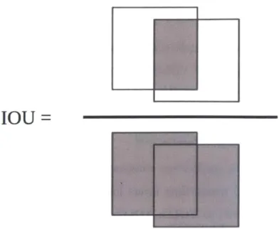
Another change from YOLO, is that YOLOv2 uses anchor boxes, or priors, over bounding box shapes and sizes, similar to Faster R-CNN [58] and SSD [42]. Using anchor boxes slightly decreases the mAP of the network from 69.5 to 69.2, but the recall shows a larger increase going from 81% to 88%. To incorporate the anchor boxes, YOLOv2 has a nominal input size of 416 x 416 so that the output feature map is 13 x 13. Having an odd-sized feature map ensures that there is an anchor box in the center of the image where, in many datasets, an object is located. Although anchor boxes were similarly used in other methods, the authors of YOLOv2 made some notable differences. For one, Faster R-CNN and SSD use hand-picked anchor boxes, whereas YOLOv2 finds its anchor boxes by running k-means clustering on the training data ground truth boxes. The clustering is done using the distance function in Equation 3.1, where d is the calculated distance and IOU is the intersection over union. The intersection over union is the ratio of the area of the intersecting region between two bounding boxes and the total area of the intersecting bounding boxes as shown in Figure 3-1. This distance formulation creates equal weighting for small and large boxes. The authors choose k = 5 for the k-means clustering. They show that with k = 5, the network achieves similar performance to methods that use 9 anchor

IOU =

Figure 3-1: The intersection over union between two bounding boxes is found by dividing the area of the intersecting region of the boxes by the total area of the boxes.

boxes. Additionally, using anchor boxes causes the spatial, and class and objectness predictions to be separated. For the case of both YOLO and YOLOv2, objectness is the IOU of the predicted bounding box and the ground truth bounding box and the class prediction is given by the conditional probability of an object of that class residing in the given bounding box given that the bounding box contains an object.

d(box, centroid) = 1 - IOU(box, centroid) (3.1)

An additional difference between the implementations of Faster R-CNN and SSD, and YOLOv2, is that instead of predicting anchor box offsets, YOLOv2 predicts bounding box coordinates relative to the anchor box cell location. Also, the bounding box size is made relative to the image size. This constrains the ground truth boxes to be within 0 and 1 and the network output is also constrained to be between 0 and 1 using a logistic activation. The detection output is given by the following equations:

r

-I

E

YOLOv2

b,= p,)a+a,

b, = ( p,) +a, bw = awe'w

bb=ahe

P

b,= px-aw+ax

b,= p,-ah+a,

bh=ahep

Figure 3-2: Anchor boxes, in green, are used as priors for predicting bounding boxes. The equations for producing the bounding box coordinates for YOLOv2 and SSD are shown on the right.

by = o-(py) + ay (3.3)

b = awePw (3.4)

bh = ahePh (3.5)

Pr(object) -IOU(b, object) = -(p,) (3.6)

where b, and by are the centers of the predicted bounding box, bw and bh are the width and height of the predicted bounding box, a, and ay are the image coordinate centers of the anchor box center, aw and ah are the anchor box's width and height,

b is the predicted bounding box, a is the logistic activation function, and px, py, pw, Ph, and p0 are the outputs of the network. An example of anchor boxes on a feature map is shown in Figure 3-2.

0

i ah

YOLOv2 uses a passthrough layer to incorporate a feature map layer with a resolution of 26 x 26 to help find objects of different sizes. The passthrough layer stacks adjacent features into different channels matching the 13 x 13 size. The base feature extractor, Darknet-19, requires almost a fourth of the floating point operations than the VGG-16 [64] base network used by Faster R-CNN at a slight cost of 2% accuracy on ImageNet.

YOLOv2 also has a useful feature in that it is trained to work with input images of different sizes. This adaptability of input size allows trade-off between speed and accuracy. The inference time decreases with lower resolution images at the cost of some accuracy. The authors train YOLO2 on images ranging from 320 x 320 to 608 x 608 with multiples of 32 in between. In this evaluation, we only tested YOLOv2 at its default 416 x 416 input size.

Another feature not explored in our evaluation of the network, is that when YOLOv2 is incorporated with a variable loss function and a tree version of Word-Net called WordTree, the network can be trained on both detection and classification datasets. The training process uses a hierarchical tree of object classes and only back-propagates the classification loss when the input to the network is from a classi-fication dataset and back-propagating the full loss when the input is from a detection dataset.

3.2

Tiny YOLO

Tiny YOLO is a faster version of the YOLOv2 network. It gains this speed at a cost to its accuracy, decreasing from a reported 76.8 mAP for YOLOv2 to 57.1 mAP on the 2007 test set [541. Tiny YOLO is derived from the Darknet reference network [55]. The Darknet reference network has similar top 1 and top 5 ImageNet classification as the AlexNet network

[38]

with only 1/10 of the parameters. Tiny YOLO uses the first seven convolutional layers and six max pooling layers from the Darknet network. This is much shallower compared to the 18 layers of the base network used by YOLOv2. Additionally, Tiny YOLO only has one added 3 x 3 convolutional layer followed by

a 1 x 1 convolutional layer compared the YOLOv2's three added 3 x 3 layers. These reductions in size make Tiny YOLO fast, but also less accurate. Despite the drop in accuracy, this lightweight network made a good candidate for our system and we chose to include it in our evaluation.

3.3

The Single Shot MultiBox Detector (SSD)

The other network architecture we evaluated was the Single Shot MultiBox Detector also known as SSD created by Liu et al. [42]. SSD, like YOLO and YOLOv2, was designed to be fast. SSD uses a base classification network followed by convolution layers of different sizes for multiscale detections. SSD uses these added layers, whereas YOLOv2 has a passthrough layer to use features from a previous feature map.

Predictions are made from these added layers by applying a 3 x 3 x p kernel, where p is the number of channels at each cell in the feature layer. Again, like Faster R-CNN and YOLOv2, SSD uses anchor boxes of different scales and aspect ratios at each feature map cell. The network then predicts anchor box offsets, as opposed to YOLOv2's cell-relative bounding box coordinates, and class confidence scores for every anchor box in each cell. The class scores for each anchor box correspond to confidence of the presence of that class in the anchor box. Along with the four bounding box offsets, this is a total of (c + 4)k outputs for each cell where k is

the number of anchor boxes per cell. The equations for finding the bounding box coordinates are given by:

bX = px aw + ax (3.7)

by = P- ah + ay (3.8)