Innovative x-ray diagnostic for impurity transport on ITER

(1)

HAL Id: tel-03153486

https://hal.archives-ouvertes.fr/tel-03153486

Submitted on 26 Feb 2021

HAL is a multi-disciplinary open access archive for the deposit and dissemination of sci-entific research documents, whether they are pub-lished or not. The documents may come from teaching and research institutions in France or abroad, or from public or private research centers.

L’archive ouverte pluridisciplinaire HAL, est destinée au dépôt et à la diffusion de documents scientifiques de niveau recherche, publiés ou non, émanant des établissements d’enseignement et de recherche français ou étrangers, des laboratoires publics ou privés.

Innovative x-ray diagnostic for impurity transport on

ITER

Colette Damien

To cite this version:

Colette Damien. Innovative x-ray diagnostic for impurity transport on ITER. Plasma Physics [physics.plasm-ph]. Aix-Marseille Université, 2021. English. �tel-03153486�

(2)

NNT/NL : 2021AIXM0019/002ED352

PhD THESIS

Soutenue à Aix-Marseille Université

le 11 janvier 2021 par

Damien COLETTE

Titre de la thèse:

Étude du transport d'impuretés sur ITER et du choix de

diagnostics X innovants associé

Discipline

Physique et Sciences de la Matière

Spécialité

Énergie, rayonnement et plasma

École doctorale

École doctorale 352 : Physique et Sciences de la Matière

Laboratoire/Partenaires de recherche

InstitutdeRecherchesurlaFusionparconfinement Magnétique, CEA Cadarache

ITER Organization

Composition du jury

Clemente ANGIONI Rapporteur IPP Garching

Marek SCHOLZ Rapporteur IFJ-PAN

Didier MAZON Directeur de thèse IRFM, CEA Cadarache

Robin BARNSLEY Examinateur ITER Organization

Conrad BECKER Examinateur Aix-Marseille Université

Sehila GONZALEZ DE

VI-CENTE Examinatrice

IAEA

Geert VERDOOLAEGE Examinateur Ghent University

(3)

Je soussigné, Damien Colette, déclare par la présente que le travail présenté dans ce manuscrit est mon propre travail, réalisé sous la direction scientifique de Didier Mazon, dans le respect des principes d’honnêteté, d’intégrité et de responsabilité inhérents à la mission de recherche. Les travaux de recherche et la rédaction de ce manuscrit ont été réalisées dans le respect à la fois de la charte nationale de déontolo-gie des métiers de la recherche et de la charte d’Aix-Marseille Université relative à la lutte contre le plagiat.

Ce travail n’a pas été précédemment soumis en France ou à l’étranger dans une version identique ou similaire à un organisme examinateur.

Fait à Cadarache le 22/10/2020

Cette œuvre est mise à disposition selon les termes de laLicence Creative Commons Attribution - Pas d’Utilisation Commerciale - Pas de Modification 4.0 International.

(4)

Résumé

La grande majorité de l’énergie mondiale provient de la combustion de combustibles fossiles. Les réserves de ces combustibles ont atteint un niveau critique ces dernières années et leur combustion émet des gaz à effets de serre, qui sont les principaux responsables du dérèglement climatique. Il est donc impératif de trouver des sources d’énergies propres et durables pour remplacer ces combustibles fossiles. La fusion thermonucléaire contrôlée est un candidat de choix. Le tokamak ITER a pour objec-tif de démontrer la faisabilité d’un réacteur de fusion générant plus d’énergie qu’il n’en consomme (Q>10). Les composants face au plasma d’ITER seront à l’origine d’une pollution de ce dernier par des impuretés lourdes telles que le tungstène. Ces impuretés sont à l’origine d’importantes pertes radiatives dans la gamme des rayons X dont la mesure est nécessaire pour étudier le transport de ces impuretés et, à terme, pouvoir identifier des actuateurs permettant de limiter leur propagation jusqu’au cœur du plasma. L’environnement radiatif d’ITER limite le choix de détecteurs X aux seuls détecteurs à gaz, dont le LVIC (Low Voltage Ionization Chamber) est le candidat principal. Cette thèse a pour but l’étude des capacités du LVIC pour la mesure de rayons X sur ITER. Un diagnostic synthétique est adapté à partir du GEM (Gas Electron Multiplier) afin de simuler la mesure par ce détecteur. L’inversion tomographique de l’émissivité X à l’aide de LVIC est étudiée et des lignes de visées additionelles, com-patibles avec les contraintes d’intégration sur ITER, sont proposées. La possibilité de discriminer le flux X en énergie est investiguée à travers une modification inno-vante du détecteur. Une méthode d’inversion basée sur la méthode des moindres carrés est spécifiquement développée pour la déconvolution du spectre X. Le profil de température électronique du plasma est extrait du spectre X avec succès. La capacité d’étude du transport d’impuretés du LVIC est démontrée à travers la reconstruction des coefficients de convection et de diffusion du tungstène d’un plasma ITER.

(5)

Abstract

The vast majority of the energy consumed in the world is coming from burning fossil fuels. The natural reserves of these fuels have reached a critical level in the last years and their combustion releases greenhouse effect gases, which are the main cause for global warming. It is therefore crucial to develop clean and sustainable energy sources in order to replace fossil fuels. Controlled thermonuclear fusion is one of the main candidates. The ITER tokamak aims at demonstrating the feasibility of a fusion reactor generating more energy than it consumes (Q>10). The ITER plasma facing components will be the source of pollution by heavy impurities such as tungsten in the plasma. Such impurities lead to great radiative losses in the X-ray range. X-ray measurement is mandatory for impurity transport studies in order to, with time, be able to identify actuators preventing impurity accumulation in the plasma core. The ITER radiative environment limits the choice of X-ray detectors to gas detectors, of which the LVIC (Low Voltage Ionization Chamber) is the most promising candidate. This thesis aims at studying the capabilities of the LVIC for X-ray measurement on ITER. A synthetic diagnostic tool has been adapted from the GEM (Gas Electron Multiplier) in order to simulate the measurement with an LVIC. Tomographic inversion of the X-ray emissivity using LVIC is studied and additional lines-of-sight, compliant with the ITER integration constraints, are proposed. The possibility of energy discrimination is investigated through an innovative modification of the detector. An inversion method based on the least squares method is specifically developed to deconvolute the X-ray spectrum. The electron temperature profile is successfully extracted from the X-ray spectrum. The capability of impurity transport study of the LVIC is demonstrated through the reconstruction of the tungsten convection and diffusion coefficients of an ITER plasma.

(6)

Remerciements

Je souhaiterai commencer par remercier Didier Mazon, Mike Walsh, Robin Barnsley et Antoine Sirinelli pour m’avoir donné l’opportunité de travailler sur ce projet.

La thèse est un travail d’équipe et je n’aurai pu rêver meilleur coéquipier que mon directeur de thèse, Didier Mazon. Merci pour ta supervision bienveillante, tes conseils, et nos conversations. Tu as toujours été là pour moi, à n’importe quelle heure de la semaine ou du weekend.

Je souhaiterai aussi remercier Robin Barnsley pour son aide. Thank you Robin for your guidance, for sharing your enthusiasm for science and diagnostics. I enjoyed every one of our chats which made me feel like a kid in a sandbox, thrilled at the thought of all the possibilities ahead of him.

Axel Jardin m’a énormément aidé lors de ces trois années et je ne saurai l’en remer-cier assez. La plupart de mon travail a été rendue possible grâce à tes conseils. Merci aussi pour ton amitié et pour ces déplacements à Garching.

J’adresse une mention spéciale à un petit poisson rouge sans mémoire, nommé Anastasia. You are by far my biggest inspiration and I feel blessed to have you in my life. This thesis is yours as well as mine, because I would not have made it without your incredible support (and cakes !).

Je souhaiterai remercier Matthieu Simeoni qui avant d’être un collaborateur est l’un de mes plus proches amis. J’apprécie énormément la confiance que tu as en moi et je suis très heureux que l’on ait pu travailler ensemble.

Je remercie l’ensemble des membres de l’IRFM que j’ai eu l’occasion de cotoyer pendant ma thèse : Philippe (merci pour ton accueil, et nos concerts ratés - on se rattrapera après le covid !), Didier (merci beaucoup pour tes conseils), Guillaume (homme sobre et sérieux), Camille (pour ta compagnie et tes jeux de mots de qualité), Adrien (le seul toujours là pour les séances de sport Pomonesques), Elizabetta et Alejandro (pour ces épiques Catan), Flavio (seul témoin des abus dont j’ai été victime par les dames de la cantine), Christian, Laurent, Éléonore, Robin, Mathieu, Arthur, Serafina, Samuele, Raffaele, Alberto, Matteo, Julien, Emily, Julio, Jorge.

Je suis également très reconnaissant envers l’équipe diagnostics d’ITER pour son accueil, en particulier Antoine, Mike, Julie, Silvia, Artur et Raphaël. Merci aussi à Martin O’Mullane et Christian Ingesson pour leur aide et conseils techniques.

(7)

D’un point de vue personnel je souhaite remercier :

— ma famille, notamment mes parents (et beaux-parents !), frères et soeurs (et riens !)

— mes géniaux colocs pomoniens Adrien, Camille, Clément, Davide, Lucie, Mylène et Jerry

— à mes amis Matthieu, Paolo et Sébastien

— Goji, le meilleur chaton du monde (même si sa contribution au manuscrit "hgfd-solllllll" n’a pas passé la première relecture)

(8)

List of Figures

1.1 Global direct primary energy consumption as a function of time,

distin-guishing each energy source. [1, 2] . . . 26

1.2 Aston curve: binding energy per nucleon as a function of the total amount of nucleons. Figure adapted from [7] . . . 30

1.3 Cross sections of several fusion reactions. [8, 9] . . . 31

1.4 Two stellarator configurations. Left: Stellarator with two sets of coils. Reproduced from [13] Right: Stellarator with a single set of coils. Repro-duced from [14] . . . 34

1.5 Principle of the Tokamak. [15]. . . 35

1.6 Illustration of the poloidal cross-section of a tokamak. . . 36

1.7 Illustration of L and H confinement modes. . . 37

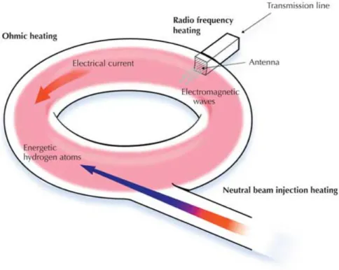
1.8 Schematic representation of the different heating sources of a toka-mak. [16] . . . 38

1.9 Left: ignition curves for different concentrations of W. Right: ignition curves for different concentrations of C. Figure adapted from [17]. . . . 39

1.10 Comparison of the Tore Supra (left) and WEST (right) poloidal cross sections. [19] . . . 40

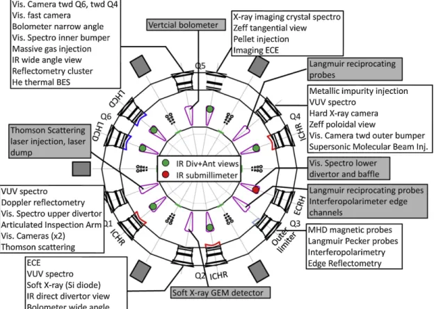
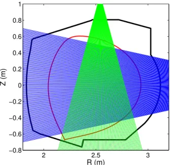
1.11 Top view of the WEST tokamak with details of its ex-vessel diagnostics. [21] 41 1.12 Poloidal cross-section view of WEST soft X-ray lines-of-sight. . . 42

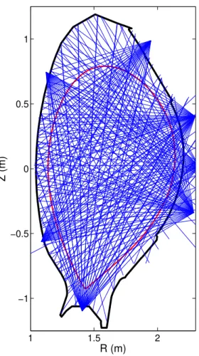
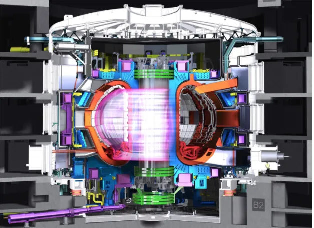
1.13 Poloidal cross-section view of ASDEX Upgrade soft X-ray lines-of-sight. 43 1.14 Drawing of the ITER tokamak and integrated plant system. . . 44

1.15 Preliminary drawing of Korea’s version of DEMO: K-DEMO. . . 46

2.1 Electronic radiation spectrum from microwaves to gamma-rays. . . 50

2.2 Atomic processes leading to X-ray emission in a plasma. . . 51

2.3 Left: Bremsstrahlung radiation spectrum of hydrogen for different elec-tron temperatures. Right: Radiative recombination spectrum of hydro-gen for different electron temperatures. . . 52

2.4 Influence of transport on the density of ions of charge z in ground state in the case of unidirectional transport along the x direction and no source term. . . 60

2.5 Cooling factors of hydrogen and tungsten as a function of Te. The W and H coefficients are taken from the open ADAS database. [32] . . . 61

2.6 Electron temperature (left) and density (right) profiles of the ITER 15MA baseline inductive scenario. . . 62

(13)

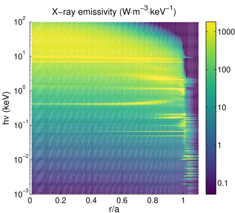
2.7 Radiated power profile as a function of photon energy and normalized radius for the standard high power D-T scenario. . . 63 2.8 Radiated power profile as a function of photon energy and normalized

radius for the standard high power D-T scenario, in the case of a hydro-gen plasma with 10−3% of tungsten. Left: Radiated profile with impurity transport. Right: Radiated profile without impurity transport. . . 64 3.1 Sketch of a semiconductor p-n junction, with bias voltage VB. The upper

part of the figure shows the energy of the valence and conduction bands and the lower part shows a schematic representation of the p-n junction. 70 3.2 Spectral response of the Si semiconducting diodes used on the tokamak

WEST. The filter consists of a beryllium window of 50µm. . . . 71 3.3 Schematic representation of a vacuum photodiode.. . . 72 3.4 Schematic representation of an ionization chamber. . . 74 3.5 Pulse size (number of charges collected) as a function of the electric

field in a chamber irradiated byα, β, and X-ray particles. The different regions of operations of the detector are as follows: recombination re-gion (I), ionization chamber rere-gion (II), proportional rere-gion (III), limited proportionality region (IV), Geiger-Müller region (V) and continuous discharge region (VI). Figure reprinted from [59] with data from [60]. . 75 3.6 Schematic representation of two pixels of a LVIC. . . 76 3.7 Mean free path as a function of energy for photons in argon and xenon

at T = 300K and P = 1bar . Cross-sections data was extracted from the NIST XCOM database [63]. . . 77 3.8 Schematic representation of a MA-LVIC with two anodes. . . 78 3.9 Spectral response for an argon-filled LVIC with five anodes. The length

pressure products of the sub-chambers are respectively 5, 15, 50, 175, and 500 mm · atm and the filter consists of 200µm of beryllium. . . . . 79 3.10 Schematic representation of a GEM detector with one GEM foil. . . 79 3.11 Possible solutions to a tomographic inversion in a 3x3 pixels space with

6 line-integrated measurements in the horizontal and vertical directions. 82 3.12 Transmission through the beryllium window (TB e), absorption in the

photodiode (Ad i od e) and spectral response (η) of AUG photodiodes with

75µm of beryllium window. . . . 84

3.13 Left: electron density as a function of time and normalised radius for AUG shot #32773. Right: electron temperature as a function of time and normalised radius for AUG shot #32773.. . . 85 3.14 Left: simulated SXR emissivity measured by the detector as a function of

time and normalised radius for AUG shot #32773. Right: experimental ed SXR emissivity measured by the detector as a function of time and normalised radius for AUG shot #32773.. . . 85

(14)

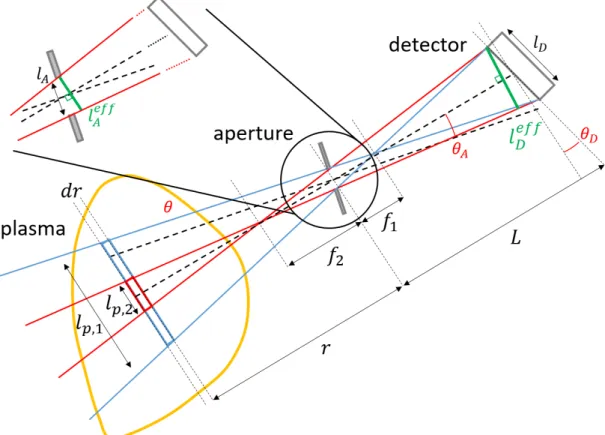
4.1 3D layout of a detector-aperture system in the case of rectangle detector and apertures. . . 88 4.2 2D layout of a detector-aperture system in a poloidal section of the plasma. 89 4.3 Sketch of a discretized poloidal cross-section of a tokamak. . . 91 4.4 Different stages of the photoionization process: (a) absorption of the

incoming photon and ionization of the electron, (b) excited ion, (c) de-excitation through X-ray fluorescence, (d) de-de-excitation through Auger electron emission . . . 92 4.5 Different stages of photon disintegration: (a) absorption of the photon

by the nucleus, (b) emission of a nucleon, (c) de-excitation throughγ-ray emission. . . 93 4.6 Different stages of Compton scattering: (a) collision between the

inci-dent photon and an electron, (b) the electron is ionized and the photon is deviated. . . 94 4.7 Different stages of Thomson scattering: (a) absorption of the photon

by the electron, (b) forced oscillation of the electron, (c) emission of a photon of same energy and different direction. . . 94 4.8 Different stages of Rayleigh scattering: (a) absorption of the photon by

the electron cloud, (b) in phase oscillations of the electrons, (c) emission of a photon of same energy and different direction. . . 95 4.9 Different stages of pair production: (a) conversion of the photon into an

electron-positron pair, (b) annihilation of the positron with an electron. 95 4.10 Contribution of the different atomic processes to the total cross-section

of argon (left) and xenon (right). The upper limit of the energy range (100 keV) considered on ITER in the scope of this thesis is indicated by a red vertical line. . . 96 4.11 Left: Total cross-sections of the different elements considered as filters.

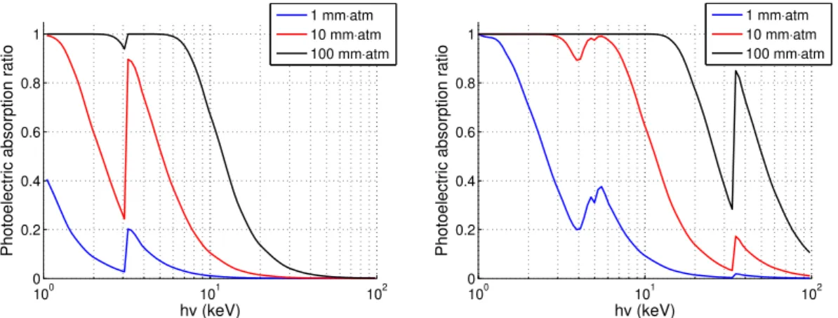
Right: Transmission ratio of different monoelement filters. . . 97 4.12 Photoelectric absorption ration for argon (left) and xenon (right) gas

detectors with different design parameter. . . 98 4.13 Architecture of the Monte Carlo-based synthetic diagnostic. Tf i l t er(hν)

denotes the transmission ratio through the filter for a photon of energy

hν, Ap−eg as(hν) denotes the photo-electric effect absorption ratio in the

gas for a photon of energy hν, P(f luorescence) is the probability of X-ray fluorescence, Ef l uor escenceis the energy of the emitted photon, W

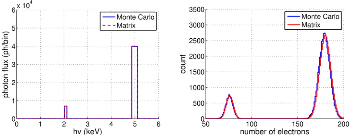
is the mean ionization energy of the gas, and F is the Fano factor of the gas. . . 100 4.14 Comparison of the monte carlo and matrix-based synthetic diagnostics.

Left: Photon flux incoming on the detectors. Right: Flux transmitted through 200µm of beryllium. . . . 103 4.15 Comparison of the monte carlo and matrix-based synthetic diagnostics.

Left: Spectrum measured by the detector, taking X-ray fluorescence into account. Right: Distribution of the charge generated by each photon. . 104

(15)

4.16 Simulation time as a function of the amount of particles simulated for the matrix and monte carlo-based synthetic diagnostic tools. . . 104 5.1 Left: ITER radial X-ray cameras in the EPP 12. Right: EPP 12 with the

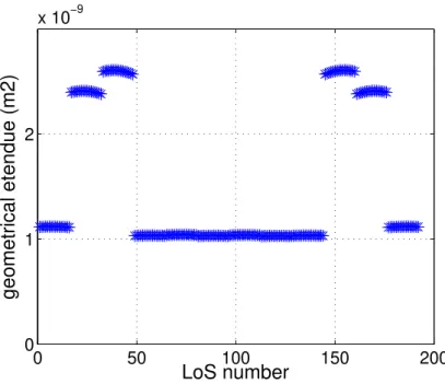
X-ray lines-of-sight.. . . 107 5.2 ITER X-ray lines-of-sight. . . 108 5.3 Geometrical etendue for each line-of-sight of the radial X-ray cameras. 109 5.4 Plasma regions considered in the computation of the figures of merit.

The pixels in the plasma core are displayed in red. The LCMS enclosed region contains both red and blue pixels. . . 110 5.5 Phantom emissivity profiles used for the assessment of the tomographic

capabilities of a lines-of-sight geometry. Upper left: gaussian profile. Upper right: hollow profile. Lower left: LFS asymmetry. Lower right: HFS asymmetry. . . 111 5.6 Phantom emissivity profile (left), tomographic reconstruction (center)

and line-integrated emissivity (right) of different emissivity configura-tions with the ITER radial X-ray cameras. First row: Gaussian emissivity profile. Second row: Hollow emissivity profile. . . 113 5.7 Phantom emissivity profile (left), tomographic reconstruction (center)

and line-integrated emissivity (right) of different emissivity configura-tions with the ITER radial X-ray cameras. First row: LFS asymmetry. Second row: HFS asymmetry. . . 114 5.8 Left: Sinogram of a tomographic system made of three sets of

lines-of-sight. Right: Geometry of the lines-of-lines-of-sight. . . 115 5.9 Left: Sinogram of the radial X-ray cameras lines-of-sight. Right:

Geome-try of the associated lines-of-sight. . . 115 5.10 Left: Sinogram of the theoretical configuration. Right: Geometry of the

associated lines-of-sight. . . 116 5.11 Phantom emissivity profile (left), tomographic reconstruction (center)

and line-integrated emissivity (right) of different emissivity configura-tions with the theoretical lines-of-sight configuration. First row: Gaus-sian emissivity profile. Second row: Hollow emissivity profile.. . . 117 5.12 Phantom emissivity profile (left), tomographic reconstruction (center)

and line-integrated emissivity (right) of different emissivity configura-tions with the theoretical lines-of-sight configuration. First row: LFS asymmetry. Second row: HFS asymmetry. . . 118 5.13 Left: Sinogram of the 60 vertical lines-of-sight configuration. Right:

Geometry of the associated lines-of-sight. . . 119 5.14 Phantom emissivity profile (left), tomographic reconstruction (center)

and line-integrated emissivity (right) of different emissivity configura-tions with the 60 vertical lines-of-sight configuration. First row: Gaus-sian emissivity profile. Second row: Hollow emissivity profile.. . . 120

(16)

5.15 Phantom emissivity profile (left), tomographic reconstruction (center) and line-integrated emissivity (right) of different emissivity configura-tions with 60 vertical lines-of-sight configuration. First row: LFS asym-metry. Second row: HFS asymasym-metry.. . . 121 5.16 Left: Sinogram of the 44 vertical lines-of-sight configuration. Right:

Geometry of the associated lines-of-sight. . . 122 5.17 Phantom emissivity profile (left), tomographic reconstruction (center)

and line-integrated emissivity (right) of different emissivity configura-tions with the 44 vertical lines-of-sight configuration. First row: Gaus-sian emissivity profile. Second row: Hollow emissivity profile.. . . 123 5.18 Phantom emissivity profile (left), tomographic reconstruction (center)

and line-integrated emissivity (right) of different emissivity configura-tions with the 44 vertical lines-of-sight configuration. First row: LFS asymmetry. Second row: HFS asymmetry. . . 124 5.19 Geometrical etendue for each 60 vertical lines-of-sight configuration. . 125 6.1 Radiated power profile as a function of photon energy and normalized

radius for the standard high power D-T scenario. . . 128 6.2 Current collected by a LVIC filled with argon (blue) or xenon (red) in the

high power D-T emissivity scenario. The chamber has a pressure length product of 50mm · atm and a filter made of 200µm of beryllium. . . . . 129 6.3 Current collected by an argon-filled (left) and xenon-filled (right) LVIC

with different filters. The chamber has a pressure length product of 50mm · atm and the emissivity comes from the high power D-T emis-sivity scenario. . . 130 6.4 Current collected by an argon-filled (left) and xenon-filled (right) LVIC

with different length pressure products. The filter is made of 200µm and the emissivity comes from the high power D-T emissivity scenario. . . 131 6.5 < η > for each channel for various incoming flux, gas, and length (for a

gas pressure of 1 bar). Top left: Xe LVIC with high power D-T scenario emissivity restricted to [0, 20] keV. Top right: Xe LVIC with high power D-T scenario emissivity up to 100 keV. Bottom left: Ar LVIC with high power D-T scenario emissivity restricted to [0, 20] keV. Bottom right: Ar LVIC with high power D-T scenario emissivity up to 100 keV. . . 133 6.6 Comparison of the reconstructed and original line-integrated plasma

emission. Left: in the full spectral range [0, 100] keV. Right: in the [0, 31] keV range. Calibrated output are obtained from Xe LVICs (50 mm · atm). The filter was made of 150µm of beryllium and 11µm of mylar. . . . 135 6.7 Comparison of the reconstructed and original line-integrated plasma

emission. Left: in the [0, 49] keV range. Right: in the [0, 23] keV range. Calibrated output are obtained from Xe (left) and Ar (right) LVICs (150

(17)

6.8 Soft x-ray emissivity profile in the [0, 20] keV range of a high power D-T ITER scenario. . . 137 6.9 Reconstruction of a soft x-ray only emissivity profile using Ar and Xe.

Top line: Tomographic reconstruction using 150 mm · atm Xe LVICs (right: reconstructed profile, left: reconstruction error). Bottom line: Tomographic reconstruction using 150 mm · atm Ar LVICs (right: recon-structed profile, left: reconstruction error). . . 139 6.10 Comparison of the tomographic reconstruction relative error and the

relative calibration error through vertical (at R = 6.59m) and radial (at Z = 0.84m) cross-sections. The x-axis coordinate of each line-of-sight corresponds to its Z-coordinate (resp: R-coordinate) at the intersection with the cross-section straight line (green line in the upper figures) in the case of the vertical (resp: radial). The upper figures display the cross-section geometry and the lower ones show the relative errors for both tomographic reconstruction and calibration. The vertical (resp: radial) cross-section plots are located on the left (resp: right) side. . . 140 6.11 Reconstruction of a soft x-ray only emissivity profile using 150 mm ·atm

Ar LVICs with ideal calibration coefficients. Right: reconstructed profile. Left: reconstruction error. . . 141 6.12 X-ray (in the [0, 100] keV range) emissivity profile of a high power D-T

ITER scenario. . . 143 6.13 Reconstruction of a wide emissivity profile using different detectors.

Left: reconstructed profile (W · m−3). Center: reconstruction error (%). Right: line-integrated emissivity and backfitting (W · m−2). Top line: 150

mm · atm LVIC filled with Xe, reconstructing the emissivity in the [0, 49]

keV range. Middle line: 50 mm · atm LVIC filled with Xe, reconstructing the emissivity in the [0, 31] keV range. Bottom line: 150 mm · atm LVIC filled with Ar, reconstructing the emissivity in the [0, 23] keV range. . . 144 6.14 Reconstruction of a wide emissivity profile with different levels of

mea-surement noise. Reconstruction over the [0, 49] keV range using xenon-filled 150 mm · atm LVIC. Top line: Tomographic reconstruction (W ·

m−3). Bottom line: Reconstruction error (%). Left column: 1% of noise. Middle column: 2% of noise. Right column: 5% of noise. . . 145 6.15 Left: Spectral response as a function of photon energy. Right: Power

impacting the detector convoluted by the spectral response and its re-construction. The detector is an argon-filled LVIC with a length pressure product of 150mm · atm and a filter made of 150µm of beryllium and

11µm of mylar. . . . 146

6.16 Left: Plasma emissivity convoluted by the spectral response of the detec-tor. Center: Tomographic reconstruction. Right: Reconstruction error. The detector is an argon-filled LVIC with a length pressure product of 150mm · atm and a filter made of 150µm of beryllium and 11µm of mylar. . . 147

(18)

6.17 Left: Spectral response as a function of photon energy. Right: Power impacting the detector convoluted by the spectral response and its re-construction. The detector is a xenon-filled LVIC with a length pressure product of 150mm · atm and a filter made of 150µm of beryllium and

11µm of mylar. . . . 148

6.18 Left: Plasma emissivity convoluted by the spectral response of the detec-tor. Center: Tomographic reconstruction. Right: Reconstruction error. The detector is a xenon-filled LVIC with a length pressure product of 150mm · atm and a filter made of 150µm of beryllium and 11µm of mylar. . . 148 7.1 Electron temperature (left) and density (right) profiles of the ITER high

power D-T scenario. . . 150 7.2 Left: Radial profile of the diffusive and convective coefficients of

tung-sten in the core negative V scenario. Right: Radial profile of the diffusive and convective coefficients of tungsten in the core positive V scenario. 151 7.3 Tungsten density as a function of time for several radial positions for the

core negative V (left) and the core positive V (right) scenarios. . . . 151

7.4 Tungsten density as a function of time and normalised radius for the

core negative V (top) and the core positive V (bottom) scenarios. . . . . 152

7.5 Tungsten density (with initial state subtracted) as a function of time and normalised radius for the core negative V (top) and the core positive V (bottom) scenarios. . . 153 7.6 Total X-ray emissivity as a function of time and normalised radius for

the core negative V (top) and the core positive V (bottom) scenarios. . . 154 7.7 X-ray emissivity spectrum at t = 1.5s at various radial positions for the

core negative V (left) and the core positive V (right) scenarios. . . . 155

7.8 Transmission ratio of a 200µm Be window, absorption ratio of a 100mm ·

at m Xe-filled LVIC, and spectral response of the combination of the two.156

7.9 Total (top) and background subtracted (bottom) X-ray emissivities con-voluted by the spectral response of the detector as a function of time and normalised radius in the case of the negative V coefficient scenario. 157 7.10 Total (top) and background subtracted (bottom) line-integrated

emis-sivities convoluted by the spectral response of the detector as a function of time and line-of-sight number in the case of the negative V coefficient scenario. . . 159 7.11 Total (top) and background subtracted (bottom) reconstructed

line-integrated emissivities convoluted by the spectral response of the de-tector as a function of time and line-of-sight number in the case of the

(19)

7.12 Total (top) and background subtracted (bottom) reconstructed X-ray emissivities convoluted by the spectral response of the detector as a function of time and normalised radius in the case of the negative V

coefficient scenario.. . . 161

7.13 Total (top) and background subtracted (bottom) reconstructed tungsten densities as a function of time and normalised radius in the case of the

negative V coefficient scenario. . . . 162

7.14ΓW/nW as a function of d nW/d t /nW for several radial positions in the

case of the negative V coefficient scenario. The dash line represents the result which would be obtained with the D and V coefficients of the scenario. . . 163 7.15 D and V coefficients of the negative V coefficient scenario and their

reconstruction. . . 163 7.16 Total (top) and background subtracted (bottom) X-ray emissivities

con-voluted by the spectral response of the detector as a function of time and normalised radius in the case of the positive V coefficient scenario. 164 7.17 Total (top) and background subtracted (bottom) line-integrated

emis-sivities convoluted by the spectral response of the detector as a function of time and line-of-sight number in the case of the positive V coefficient scenario. . . 166 7.18 Total (top) and background subtracted (bottom) reconstructed

line-integrated emissivities convoluted by the spectral response of the de-tector as a function of time and line-of-sight number in the case of the

positive V coefficient scenario.. . . 167

7.19 Total (top) and background subtracted (bottom) reconstructed X-ray emissivities convoluted by the spectral response of the detector as a function of time and normalised radius in the case of the positive V

coefficient scenario.. . . 168

7.20 Total (top) and background subtracted (bottom) reconstructed tungsten densities as a function of time and normalised radius in the case of the

positive V coefficient scenario.. . . 169

7.21ΓW/nW as a function of d nW/d t /nW for several radial positions in the

case of the positive V coefficient scenario. The dash line represents the result which would be obtained with the D and V coefficients of the scenario. . . 170 7.22 D and V coefficients of the positive V coefficient scenario and their

re-construction. . . 170 7.23 Soft x-ray radiation profiles observed for two different heating strategies

in the JET tokamak. Reprinted from [104] . . . 171 7.24 Banana-shaped orbit of a trapped particle. Figure reprinted from [105]. 172 7.25 2D tungsten density profile (left) and its reconstruction (right) in the

(20)

7.26 Tungsten density poloidal fluctuation (left) and its reconstruction (right) in the case of a symmetrical tungsten density profile. . . 175 7.27 Left: radial profile of the toroidal rotation frequency. Right: Radial profile

of the minority temperature anisotropy ratio. . . 176 7.28 Radial profile of the ion and electron temperatures.. . . 177 7.29 2D tungsten density profile (left) and its reconstruction (right) in the

case of a tungsten density profile exhibiting an electric field-induced asymmetry.. . . 177 7.30 Tungsten density poloidal fluctuation (left) and its reconstruction (right)

in the case of a tungsten density profile exhibiting an electric field-induced asymmetry. . . 178 7.31 2D tungsten density profile (left) and its reconstruction (right) in the

case of a tungsten density profile exhibiting a centrifugal force-induced asymmetry.. . . 179 7.32 Tungsten density poloidal fluctuation (left) and its reconstruction (right)

in the case of a tungsten density profile exhibiting a centrifugal force-induced asymmetry. . . 179 7.33 2D tungsten density profile (left) and its reconstruction (right) in the

case of a tungsten density profile exhibiting an asymmetry induced by both an electric field and the centrifugal force. . . 180 7.34 Tungsten density poloidal fluctuation (left) and its reconstruction (right)

in the case of a tungsten density profile exhibiting an asymmetry induced by both an electric field and the centrifugal force. . . 181 8.1 Schematics of a multi-anodes low voltage ionization chamber. . . 184 8.2 Contribution of each impurity to the incoming photon flux of

line-of-sight number 96 which goes through the very core of the plasma. . . . 185 8.3 Fitting of the line-of-sight number 96 incoming photon flux. In this

figure, the parameters of the function are X1= 1.40 · 109 ph/s, X2= 2.26 · 10−2keV−1, X3= 5.0 · 109ph/s, and X4= 6.0 · 108ph/s.. . . 186 8.4 Architecture of the minimization algorithm. . . 188 8.5 Spectral response of each sub-chamber in a 5 anodes argon-filled

MA-LVIC. The length pressure products of the sub-chamber are respectively 5, 15, 50, 175, and 500 mm · atm, and the filter consists of 200µm of beryllium. . . 190 8.6 Left: Spectral deconvolution of the photon flux of line-of-sight 45 (r /a ≈

0.5). Right: Spectral deconvolution of the photon flux of line-of-sight 96 (r /a ≈ 0). The MA-LVIC is filled with argon and the sub-chambers have respective length pressure products of 5, 15, 50, 175 and 500 mm · atm. The beryllium window is 200µm wide. . . . 190

(21)

8.7 Left: Spectral deconvolution of the photon flux of line-of-sight 5 (r /a ≈ 1). Right: Measured and reconstructed currents for each sub-chamber for lines-of-sight 5, 45 and 96. The MA-LVIC is filled with argon and the sub-chambers have respective length pressure products of 5, 15, 50, 175 and 500 mm · atm. The beryllium window is 200µm wide.. . . 191 8.8 Left: Figures of merit of spectral deconvolution. Right: Spectral

decon-volution of the photon flux of line-of-sight 4 (r /a ≈ 1). The MA-LVIC is filled with argon and the sub-chambers have respective length pressure products of 5, 15, 50, 175 and 500 mm · atm. The beryllium window is

200µm wide. . . . 192

8.9 Left: Surface integrated power as a function of the photon energy and the line-of-sight number. Right: Reconstructed surface integrated power as a function of the photon energy and the line-of-sight number. The MA-LVIC is filled with argon and the sub-chambers have respective length pressure products of 5, 15, 50, 175 and 500 mm · atm. The beryllium window is 200µm wide. . . . 193 8.10 Left: Reconstruction of the line-integrated X-ray emissivity in the [2,

3] keV range for each of-sight. Right: Reconstruction of the line-integrated X-ray emissivity in the [6, 10] keV range for each line-of-sight. The MA-LVIC is filled with argon and the sub-chambers have respective length pressure products of 5, 15, 50, 175 and 500 mm · atm. The beryllium window is 200µm wide. . . . 193 8.11 Left: Reconstruction of the line-integrated X-ray emissivity in the [10,

100] keV range for each of-sight. Right: Reconstruction of the line-integrated X-ray emissivity in the [2, 100] keV range for each line-of-sight. The MA-LVIC is filled with argon and the sub-chambers have respective length pressure products of 5, 15, 50, 175 and 500 mm · atm. The beryllium window is 200µm wide. . . . 194 8.12 Spectral response of each sub-chamber in a 5 anodes xenon-filled

MA-LVIC. The length pressure products of the sub-chamber are respectively 5, 30, 60, 100 and 150 mm · atm, and the filter consists of 200µm of beryllium. . . 195 8.13 Left: Spectral deconvolution of the photon flux of line-of-sight 45 (r /a ≈

0.5). Right: Spectral deconvolution of the photon flux of line-of-sight 96 (r /a ≈ 0). The MA-LVIC is filled with xenon and the sub-chambers have respective length pressure products of 5, 30, 60, 100 and 150 mm · atm. The beryllium window is 200µm wide. . . . 196 8.14 Left: Spectral deconvolution of the photon flux of line-of-sight 5 (r /a ≈

1). Right: Measured and reconstructed currents for each sub-chamber for lines-of-sight 5, 45 and 96. The MA-LVIC is filled with xenon and the sub-chambers have respective length pressure products of 5, 30, 60, 100 and 150 mm · atm. The beryllium window is 200µm wide.. . . 196

(22)

8.15 Left: Figures of merit of spectral deconvolution. Right: Spectral decon-volution of the photon flux of line-of-sight 4 (r /a ≈ 1). The MA-LVIC is filled with xenon and the sub-chambers have respective length pressure products of 5, 30, 60, 100 and 150 mm · atm. The beryllium window is

200µm wide. . . . 197

8.16 Left: Surface integrated power as a function of the photon energy and the line-of-sight number. Right: Reconstructed surface integrated power as a function of the photon energy and the line-of-sight number. The MA-LVIC is filled with xenon and the sub-chambers have respective length pressure products of 5, 30, 60, 100 and 150 mm · atm. The beryllium window is 200µm wide. . . . 197 8.17 Left: Reconstruction of the line-integrated X-ray emissivity in the [2,

3] keV range for each of-sight. Right: Reconstruction of the line-integrated X-ray emissivity in the [6, 10] keV range for each line-of-sight. The MA-LVIC is filled with xenon and the sub-chambers have respective length pressure products of 5, 30, 60, 100 and 150 mm · atm. The beryllium window is 200µm wide. . . . 198 8.18 Left: Reconstruction of the line-integrated X-ray emissivity in the [10,

100] keV range for each of-sight. Right: Reconstruction of the line-integrated X-ray emissivity in the [2, 100] keV range for each line-of-sight. The MA-LVIC is filled with xenon and the sub-chambers have respective length pressure products of 5, 30, 60, 100 and 150 mm · atm. The beryllium window is 200µm wide. . . . 199 8.19 Reconstruction of the line-integrated X-ray emissivity in the [2, 3] keV

range as a function of the line-of-sight number for different widths of the beryllium window. The MA-LVIC is filled with xenon and the sub-chambers have respective length pressure products of 5, 30, 60, 100 and 150 mm · atm. . . . 200 8.20 Left: R M Sd ec and its 1% noise envelope. Right: Reconstruction of the

line-integrated X-ray emissivity in the [2, 3] keV energy range and its 1% envelope. The MA-LVIC is filled with xenon and the sub-chambers have respective length pressure products of 5, 30, 60, 100 and 150 mm · atm. The beryllium window is 200µm wide. . . . 201 8.21 Left: Reconstruction of the line-integrated X-ray emissivity in the [6, 10]

keV energy range and its 1% envelope. Right: Reconstruction of the line-integrated X-ray emissivity in the [10, 100] keV energy range and its 1% envelope. The MA-LVIC is filled with xenon and the sub-chambers have respective length pressure products of 5, 30, 60, 100 and 150 mm · atm. The beryllium window is 200µm wide. . . . 202

(23)

8.22 Left: Radiated power profile on ITER as a function of photon energy and normalized radius. Right: Reconstructed radiated power profile as a function of photon energy and normalized radius. The MA-LVIC is filled with xenon and the sub-chambers have respective length pressure products of 5, 30, 60, 100 and 150 mm · atm. The beryllium window is

200µm wide. . . . 204

8.23 Left: Figures of merit of energy resolved tomography: R M Sl i ne, R M Sl cmst omo,

and R M Scor e_{t omo}. Right: Reconstruction of the local plasma emissivity in the plasma core (at R = 6.27m and Z = 0.57m). For this pixel, R M Spi x=

3.7 · 10−3. The MA-LVIC is filled with xenon and the sub-chambers have respective length pressure products of 5, 30, 60, 100 and 150 mm · atm. The beryllium window is 200µm wide. . . . 204 8.24 Figure of merit R M Spi x of energy resolved tomography. The MA-LVIC is

filled with xenon and the sub-chambers have respective length pressure products of 5, 30, 60, 100 and 150 mm · atm. The beryllium window is

200µm wide. . . . 205

8.25 Left: Reconstruction of the local emissivity spectrum in the plasma core (at R = 6.27m and Z = 0.57m) with 1% of perturbative noise added to the measurement. Right: Figures of merit of energy resolved tomography:

R M Sl i ne, R M SLC M St omo and R M Scor et omo (respectively labelled as F OMLoS,

F OMl cms, and F OMcor e), with 1% of gaussian perturbative noise on

the LVIC measurement. The MA-LVIC is filled with xenon and the sub-chambers have respective length pressure products of 5, 30, 60, 100 and 150 mm · atm. The beryllium window is 200µm wide. . . . 206 8.26 Left: Figure of merit R M Spi x of energy resolved tomography with 1%

of gaussian perturbative noise on the LVIC measurement computed in the [4, 10] keV range. Right: Figure of merit R M Spi x of energy resolved

tomography with 1% of gaussian perturbative noise on the LVIC mea-surement computed in the [10, 100] keV range. The MA-LVIC is filled with xenon and the sub-chambers have respective length pressure prod-ucts of 5, 30, 60, 100 and 150 mm ·atm. The beryllium window is 200µm wide. . . 207 8.27 Left: 2D profile of the electron temperature in the ITER high power D-T

scenario. Right: Reconstructed 2D profile of the electron temperature. The MA-LVIC is filled with xenon and the sub-chambers have respec-tive length pressure products of 5, 30, 60, 100 and 150 mm · atm. The beryllium window is 200µm wide. . . . 208 8.28 Relative error of the electron temperature reconstruction. The

MA-LVIC is filled with xenon and the sub-chambers have respective length pressure products of 5, 30, 60, 100 and 150 mm · atm. The beryllium window is 200µm wide. . . . 209

(24)

8.29 Left: Reconstructed electron temperature profile obtained after energy resolved tomography with 1% of gaussian perturbative noise on the LVIC measurement. Right: Relative error of the electron temperature reconstruction with 1% of gaussian perturbative noise on the LVIC mea-surement. The MA-LVIC is filled with xenon and the sub-chambers have respective length pressure products of 5, 30, 60, 100 and 150 mm · atm. The beryllium window is 200µm wide. . . . 210

(25)

List of Tables

1.1 Parameters of the WEST tokamak. . . 41 1.2 Parameters of the ASDEX Upgrade tokamak. . . 43 1.3 Parameters of the ITER tokamak. . . 45 1.4 Parameters of the European version of the DEMO tokamak. . . 45 5.1 Figures of merit for tomographic reconstruction of phantom emissivity

profiles with the radial X-ray cameras.. . . 112 5.2 Figures of merit for tomographic reconstruction of phantom emissivity

profiles with the theoretical lines-of-sight configuration.. . . 117 5.3 Figures of merit for tomographic reconstruction of phantom emissivity

profiles with the 60 vertical lines-of-sight configuration. . . 122 5.4 Figures of merit for tomographic reconstruction of phantom emissivity

profiles with the 44 vertical lines-of-sight configuration. . . 123 6.1 Figures of merit for tomographic reconstruction over [0, 20] keV. . . 137 6.2 Figures of merit for tomographic reconstruction over [0, 100] keV. . . . 143 6.3 Figures of merit for the noise study. . . 145 6.4 Figures of merit for tomographic reconstruction of the emissivity

(26)

1 Introduction

Sommaire

1.1 The challenge of energy . . . 25 1.1.1 Historical approach . . . 25 1.1.2 Fossil fuels: availability and consequences . . . 26 1.1.3 Alternative energy sources . . . 27 1.1.4 Energy generation from nuclear fusion . . . 28 1.2 Nuclear fusion reactor . . . 29 1.2.1 Fusion reactions . . . 30 1.2.2 Ignition . . . 31 1.2.3 Confinement . . . 33 1.2.3.1 Gravitational confinement . . . 33 1.2.3.2 Inertial confinement . . . 33 1.2.3.3 Magnetic confinement . . . 33 1.2.4 Tokamak . . . 35 1.2.4.1 Geometry . . . 35 1.2.4.2 Confinement modes . . . 36 1.2.4.3 Heating . . . 37 1.2.4.4 Key challenges . . . 38 1.2.5 Existing tokamaks . . . 40 1.2.5.1 WEST. . . 40 1.2.5.2 ASDEX Upgrade . . . 42 1.2.5.3 ITER . . . 44 1.2.5.4 DEMO . . . 45 1.3 Scope of this thesis . . . 46

1.1 The challenge of energy

1.1.1 Historical approach

Energy is a physical quantity which characterises the ability of a system to produce work, which describes the change of state (e.g. position, speed, heat, pressure) of said system. In other words, energy reflects the ability of mankind to master (or transform) its environment: energy is what allows us to eat, heat our homes, travel or charge our computers.

(27)

Figure 1.1 – Global direct primary energy consumption as a function of time, distin-guishing each energy source. [1,2]

Throughout most of mankind history, the amount of energy available was mostly limited to wood (for heating) and animals (mainly for transportation or field labour). These two sources are the so-called traditional biomass displayed on figure1.1. The invention of the steam engine by James Watt at the end of the eighteenth century allowed mankind to extend its energy consumption through the use of machines. The first energy source used to power engines is coal, followed by oil which made its appearance in the nineteenth century. Other energy sources such as gas, nuclear, hydro or solar have been domesticated in the twentieth century. This abundance of energy has permitted mankind to shape the world as we know it. It can be noted on figure1.1that the world energy consumption has been rising constantly for the last 200 years, and this rise is expected to keep on. [3] In this section, the energy challenge is addressed through energy generation but it should be kept in mind that an increase in energy efficiency and a more efficient use of energy (e.g. limiting waste, public transportation, better house thermal isolation, consumption of local products) are also key to solving the energy challenge.

1.1.2 Fossil fuels: availability and consequences

Fossil fuels are the remains of the decomposition of organic matter such as dead or-ganisms. Their creation occurred on the scale of millions of years, and therefore it can be considered that the world reserves of fossil fuel are constant. Three different fossil fuels (coal, oil, gas) are currently used to generate more than 80% of the world energy.

(28)

Energy is generated by oxidation of the fuel, which is achieved through combustion. The current reserves of coal are estimated to last around 130 years at the current rate. In the case of oil, the proven reserves should allow 50 to 60 years of energy at the cur-rent rate. Gas offers 90 years of energy if there is not increase of energy consumption. It can be seen on figure1.1that energy demand has been increasing fairly linearly in the 1950-2019 interval and this is likely to keep on. New fossil fuel discoveries are therefore necessary in order to keep on using fossil fuel for up to 130 years. In the scale of human history, such duration is however very limited and fossil fuels cannot be considered as a long-term energy source.

Availability is not however the only limitation to the use of fossil fuels, their impact on the environment and on health should also be considered. [4] Extraction of fossil fuels (whether it is underground or at the surface) leads to extensive land degradation, water pollution and gas emissions (benzene and formaldehyde). These can lead to health hazards, both on minors and the population. The combustion of these fuels in order to create energy releases harmful particles in the atmosphere which lead to an increase in acid rains and respiratory illnesses. The main issue regarding fossil fuels is the release of greenhouse effect gases which participate in the human-induced global warming of the world. The consequences of global warming include an increase in the frequency and intensity of extreme meteorological events (e.g. floods, droughts, hurricanes), rising of the sea level (jeopardizing most coastline cities), ice melting in the poles and biodiversity extinction.

In conclusion on fossil fuels, current reserves would only allow the current energy production for up to around a hundred years. However if climate change is to be mitigated to bearable limits both for the environment and our society, most of the remaining fossil fuel should remain underground.

1.1.3 Alternative energy sources

We are now facing a challenge requiring a shift in the energy mix if we are to limit global warming. Several energy sources can be considered as potential alternatives to fossil fuel. So-called renewable sources of energy have the main advantage that their availability is not limited in time as they are constantly renewed.

Wind and solar power are the first examples of renewable energy which come to mind. Electricity can be generated by adding a generator to a windmill or by using photo-voltaic panels which convert light into electrons. These processes are not very energy efficient, but do not release greenhouse effect gases during operation. However their production and maintenance is quite costly in terms of energy and the greenhouse effects gases released in the process should be taken into account. Both sources depend on the weather and are therefore intermittent and not controllable. Their production peaks do not necessarily coincide with the demand peaks. As a result, a controllable source is required in order to provide energy when wind and/or solar are not producing.

(29)

en-ergy (the rotation of a turbine) and then into electricity through the use of a generator. It is a controllable source of energy which does not release green house effect gases during operation. Its construction is quite costly but its lifetime makes the overall green house effect production very low. A dam can be used as an energy storage facility by pumping water uphill. However, the installation of a dam creates considerable changes in the environment due to the drowning of a large zone and its failure could prove deadly. The hydro power can hardly be increased in developed countries be-cause most of the areas available for dams are already exploited.

Biofuels are a promising source of energy which consists of burning oil or ethanol ob-tained from plants (e.g. rape, wheat). The combustion of biofuels leads to greenhouse effect gases emission. However, the crops where such plants are cultivated absorb carbon dioxide and therefore reduce the net greenhouse effect gases production of biofuels. These crops are in competition with food crops and the quantities of biofuel which can be produced are constrained by land availability.

Nuclear fission is another alternative to fossil fuels. It is not a renewable source of energy as the energy is extracted from a metal (uranium or plutonium) through fission reactions. Nuclear fission has the advantage that it is a controllable source of energy which is not intermittent. Approximately 100 years of reserves of235U are available, but the development of fast neutrons reactors could allow the use of238U for which 10,000 years of fuel are available. The main drawbacks of nuclear energy are safety and waste management. Accidents in nuclear power plants are extremely rare but can release a high amount of radioactive material in the atmosphere and have very serious health consequences. The fission reaction leads to the generation of hazardous waste with a very long radioactive decay time compared to human time scale. At the mo-ment, the only solution foreseen to dispose of such waste is deep burial underground. It can be seen that each alternative to fossil fuels comes with its own advantages and drawbacks. Renewable energies do not allow a massive energy production adapted to the demand, either because of fluctuating production or land occupation. They should be used in coordination with an energy source which can deliver such pro-duction. Promising candidates are fourth generation fast neutrons fission reactors, carbon-trapping thermal reactors fuelled with coal or nuclear fusion reactors.

1.1.4 Energy generation from nuclear fusion

Due to the topic of this thesis, a special focus is given on generation of energy through nuclear fusion. Fusion reactions of light elements release energy in the form of kinetic energy of the fusion products. The so-called D-T fusion reaction is the most accessible in reactor conditions. D stands for deuterium, which is the2H isotope of hydrogen, and T stands for tritium, which is the3H isotope of hydrogen. Nuclei of deuterium and tritium fuse together at high temperature in the following reaction:

(30)

whereα is a He2+ nucleus and n is a neutron. The total energy generated by a D-T reaction is∆E = 17.6MeV , which is around 8 times higher than a235U fission reaction but with reactants around 50 times lighter.

In terms of availability, nuclear fusion exhibits the advantage that deuterium is a very common isotope of hydrogen which can be extracted from seawater at a low cost. At the present energy consumption, enough deuterium can be extracted for several billions of years of electricity production. Tritium is a radioactive isotope of hydrogen with a very short decay period. The naturally generated tritium has decayed long ago and the world tritium inventory has been produced by nuclear reactions of neutrons with heavy water in nuclear reactors or with lithium. Tritium generation can be achieved in nuclear fusion power plants by surrounding the reactor with lithium blankets. This technique is called tritium breeding and requires neutron multiplication in order for the reactor to be self-sufficient tritium-wise. The availability of nuclear fusion therefore depends on lithium, for which the reserves are expected to last for a thousand years. [5] This value is subject to a high uncertainty as lithium use is massive (electronics, batteries, ...).

The environmental impact of nuclear fusion is very low compared to the energy sources listed previously. Indeed, the fusion product are neutrons and helium. Helium is an inert gas which is not radioactive. Neutrons however irradiate the fusion reactor which becomes radioactive. The decay period of a fusion reactor at the end of its lifetime is around 100 years, which is a ridiculously low duration in comparison with fission products.

Fusion reactors are inherently safe. Indeed they operate in very specific conditions, and in the case of a disruption fusion reactions just end prematurely. No reaction avalanche leading to the release of the reactor energy content in a short amount of time can therefore be observed. Due to constant fuelling of the reactor, only a small quantity of fuel is present at any given time (a couple of minutes in a fusion reactor compared to several months in a fission reactor). Moreover, the fuelling can be stopped if necessary. Even if the magnetic energy damaging the reactor, it has been demonstrated that no tritium leaking nor confinement failure is expected. [6] And in the case where the reactor is damaged by an outside event, the maximal amount of tritium released is around 1kg which should have limited consequences on health, and only in a small region and period of time.

1.2 Nuclear fusion reactor

This section describes the different aspects of nuclear fusion and how they led to the design of the tokamak.

(31)

1.2.1 Fusion reactions

The binding energy per nucleon for the different elements of the periodic table is shown on figure1.2. It reflects the stability of an atom: the higher the binding energy per nucleon the more stable the atom. One can notice that iron (56F e) is the most stable element in the table. Heavier elements can become more stable by splitting into lighter elements and lighter elements can become more stable by merging into heavier elements. These two processes are respectively nuclear fission and nuclear fusion. When the products of a nuclear reaction are more stable than the reactants, energy is released (usually in the shape of kinetic energy or radiation).

Figure 1.2 – Aston curve: binding energy per nucleon as a function of the total amount of nucleons. Figure adapted from [7]

The slope of the Aston curve denotes the gain of energy per nucleon. It is clear that fusion reactions of hydrogen isotopes into helium are the most energy-efficient reactions. Nuclear reactions are defined by their cross-sections, which describes the probability of occurrence of such reactions and are usually expressed in barns: 1b = 10−28m2. The cross-sections of the main candidates for power generation from nuclear fusion are displayed on figure1.3. It can be clearly seen that the D-T fusion reaction (see equation1.1) is the most likely to take place in a fusion reactor below several hundreds keV. The D-T reaction reaches its peak cross-section at E ≈ 100keV , which corresponds to T ≈ 109K with E = kB· T (1eV → 11594K ). In plasma physics, it

is common for temperatures to be expressed in electron-volts and to refer to kB· T . It

(32)

101 102 103 104 10−4 10−3 10−2 10−1 100 101 Energy (keV) Cross section (b) D−T D−3He D−Dn D−Dp

Figure 1.3 – Cross sections of several fusion reactions. [8,9]

In nuclear fusion reactors, the temperatures reached are of the order of 10keV only but it is sufficient to generate a significant amount of D-T reactions. High temperatures are required in order to overcome the Coulomb repulsion of D+and T+, which is achieved by tunnel effect. In such conditions, the matter only exists in plasma state.

1.2.2 Ignition

The power generated by D-T reactions is given by:

P_D−T= RD−T· ∆E = nDnT < σv > ∆E (1.2)

where R_D−T is the D-T reaction rate in s−1,∆E = 17.6MeV is the energy generated by a D-T fusion reaction, nD and nT are respectively the deuterium and tritium densities

in m−3, < . > is the average over the Maxwellian velocity distribution. This power is maximised for nD= nT =n₂:

P_D−T=n

2

4 < σv > ∆E (1.3)

Each fusion product has a different destiny in the plasma, and so does their energy. Indeed, theα particle deposits its energy in the plasma through collisions while the neutron exits the plasma volume without interacting (in most cases). The energy of the neutron is therefore lost to the plasma, but can be used for electricity generation. During operation the power lost (through radiation and conduction [10]) PL must

be offset by the power incoming in the plasma PH+ Pα(PH is the heating power):

(33)

radiation losses: P_α≥ PL.

Theα heating P_αis given by:

P_α=n

2

4 < σv > Eα (1.4)

where E_α= 3.5MeV is the energy of the alpha particle.

The energy confinement time of the plasmaτE is defined as the time it would take

the plasma to lose all its energy if the energy sources were stopped:τE = W /PL. The

power losses can therefore be written as: PL=

W τE

(1.5) The local energy content of the plasma w is given by:

w =3

2(neTe+ niTi) (1.6)

where neand ni are respectively the electron and ion densities. In the case of a

hydro-gen plasma (ne= ni= n) in which electrons and nuclei have the same temperature

(Te= Ti= T ), equation1.6becomes:

w = 3nT (1.7)

In an homogeneous plasma, the power losses become: PL=

3nT τE

(1.8) During the operation of a fusion reactor the power balance is given by:

PH+ Pα= PL⇐⇒ PH+ n2 4 < σv > Eα= 3nT τE (1.9) The ignition is reached for P_α≥ PL, which gives:

n2 4 < σv > Eα≥ 3nT τE ⇐⇒ nT τE ≥ 12T2 < σv > Eα (1.10)

The triple product nTτE is an adequate indicator of the efficiency of plasma

confine-ment. The ratio _<σv>T2 has a minimal value for T = 14keV , leading to the following ignition criterion [10]:

(34)

The previous expression considers flat temperature profiles but in tokamaks the temperature profiles usually are peaked, in which case:

nTτE ≥ 5 · 1021m−3· s · keV (1.12)

The fusion amplification factor can be defined as: Q =PD−T

PH =

5 · Pα

PH

(1.13) Ignition corresponds to Q → ∞ and Q = 1 means that Pαcorresponds to 20% of the

total heating power. One of the major ITER goals is to achieve Q ≥ 10 which means that alpha particles provide more than two thirds of the total heating power.

1.2.3 Confinement

As seen in section1.2.2, confinement of the plasma is key to achieve ignition. More-over, an efficient confinement of the plasma protects the plasma facing components (PFC) from the very hot plasma and avoids cooling of the plasma on the walls of the vacuum vessel. This section describes the main confinement strategies linked to nuclear fusion.

1.2.3.1 Gravitational confinement

Gravitational confinement occurs naturally in stars. Due to their huge mass, gravita-tional forces are high enough to create conditions such that nTτE is high enough to

achieve ignition. For obvious reasons it is not possible to replicate such confinement strategy on Earth and other solutions have been developed.

1.2.3.2 Inertial confinement

Inertial confinement consists of a very high compression of deuterium and tritium for a very short time. In such conditions, temperature and density must be high enough to compensate for the short confinement time in order to reach ignition. This approach is used in H bombs where the compression is obtained by detonating a fission bomb. Another solution for such compression is the use of numerous high power lasers on a small D-T target. It is the approach used at the Laser Megajoule in France [11] and the National Ignition Facility in the USA [12]. The possibility to use such approach for energy production has not been demonstrated yet.

1.2.3.3 Magnetic confinement

Another approach for confinement is based on the fact that, at the temperatures required for ignition, the matter is in a plasma state. In a plasma electrons and ions, which are charged particles, are separated. A magnetic field can therefore be used to

(35)

confine them. Indeed, charged particles follow the helical trajectories centered on magnetic field lines due to the Lorentz force. Magnetic field lines are lines over which the magnetic field is constant (they are tangential to the magnetic field). For a particle of charge Z · |e|, mass m, velocity (orthogonal to the magnetic field) and in a magnetic field of amplitude B, the helical movement is defined by its radius and pulsation:

ρ = mV Z eB ωC = Z eB m (1.14)

The radius of the oscillation is the so-called Larmor radius and its pulsation is the cyclotron pulsation.

A reactor with linear magnetic field lines with magnetic mirrors at both ends could be an easy solution for plasma confinement. However localised instabilities (called flute instabilities due to their shape) appear at the edges of such device, leading to significant edge losses and possibly to the loss of confinement of the plasma. Another solution would be to us a torus shaped reactor with circular magnetic field lines. In such configuration, the particles would be subject to a vertical drift due to the gradient and curvature of the magnetic field. The direction of the drift depends on the charge, thus leading to the creation of an unwanted electric field in the plasma that would eject the particle out of it.

This effect can be compensated by the use of helical field lines, created by the super-position of a poloidal and toroidal magnetic field. The toroidal direction is defined as the direction following the torus and the poloidal plane is defined as the plane which is orthogonal to it. Helical magnetic field lines are achieved in two different magnetic configurations.

Figure 1.4 – Two stellarator configurations. Left: Stellarator with two sets of coils. Re-produced from [13] Right: Stellarator with a single set of coils. ReRe-produced from [14]

A first configuration consists of shaping the coils specifically in order to obtain a helical magnetic field. Such machines are called stellarators and are very complex to build. Two options are available when shaping the magnetic field: a single set of

(36)

complex non-planar coils or two different sets of simpler coils can be used. In the two sets approach, one set of coils shapes the toroidal magnetic field and the other one shapes the poloidal magnetic field.

The second approach, which is the most widely spread, is used on devices called Tokamaks (see figure1.5). In such machines, planar toroidal coils shape the toroidal magnetic field. The poloidal magnetic field results from the generation of a toroidal current in the plasma. This current is generated by the addition of a central solenoid which plays the role of the primary circuit of a transformer, the secondary circuit being the plasma. Current flowing in the primary circuit leads to the generation of a current in the secondary circuit by induction. Additional coils can be added to the tokamak to control the shape and position of the plasma.

Figure 1.5 – Principle of the Tokamak. [15]

1.2.4 Tokamak

1.2.4.1 Geometry

In order to understand the geometry of a tokamak, a poloidal cross-section of a tokamak is displayed on figure1.6. The tokamak is made of a vacuum vessel containing a plasma, the aforementionned coils, and additional systems (e.g. heating, diagnostics, pumping). The plasma is constrained in size by either a limiter or a divertor.

The limiter is simply a plasma facing component coming in tangential contact with the plasma. This leads to the opening of the magnetic surfaces located behind the limiter and therefore a restriction of the plasma to the region before the contact with the limiter. The limiter configuration leads to a significant pollution of the plasma by impurities ejected from the limiter, which affects the tokamak performance.

On the other hand, the divertor affects the magnetic topology of the Last Closed Magnetic Surface (LCMS) in order to create a so-called x-point. The x-point divides the