CFD analysis of the turbulent flow in a PWR 5x5 rod bundle with staggered structural grids

HAL Id: cea-03109325

https://hal-cea.archives-ouvertes.fr/cea-03109325

HAL is a multi-disciplinary open access archive for the deposit and dissemination of sci-entific research documents, whether they are pub-lished or not. The documents may come from teaching and research institutions in France or abroad, or from public or private research centers.

L’archive ouverte pluridisciplinaire HAL, est destinée au dépôt et à la diffusion de documents scientifiques de niveau recherche, publiés ou non, émanant des établissements d’enseignement et de recherche français ou étrangers, des laboratoires publics ou privés.

CFD analysis of the turbulent flow in a PWR 5x5 rod

bundle with staggered structural grids

Pierre-Emmanuel Angeli, Mathieu Peybernes

To cite this version:

Pierre-Emmanuel Angeli, Mathieu Peybernes. CFD analysis of the turbulent flow in a PWR 5x5 rod bundle with staggered structural grids. CFD4NRS-6 - The 6th workshop on Computational Fluid Dynamics for Nuclear Reactor Safety Applications, OCDE, Sep 2016, Cambridge, United States. �cea-03109325�

CFD ANALYSIS OF THE TURBULENT FLOW IN A PWR 5x5 ROD BUNDLE WITH STAGGERED STRUCTURAL GRIDS

P.E. Angeli, M.P. Peybernes

CEA-SACLAY, DEN/SAC/DANS/DM2S/STMF/LMSF, F-91191 Gif-sur-Yvette, France

[email protected] [email protected]

Abstract

Simulations of turbulent flow in Pressurized Water Reactor (PWR) fuel assemblies are performed with the code TrioCFD. Calculations are compared to measurements performed at the AGATE facility consisting of a 5x5 rod bundle with axially staggered grids. Measurements are carried out with the Laser Doppler Velocimetry (LDV) technique. Several turbulent modelling approaches are investigated. Two Reynolds-averaged Navier–Stokes (RANS) models (standard linear k − ε model and Non-Linear Eddy Viscosity Model) and Large Eddy Simulation (LES) are compared to the AGATE experiments. For various distances from the mixing grids, calculated vertical and horizontal profiles of the axial and cross-flow velocities are analyzed. The three turbulence models provide very similar results downstream from the grids where inertia effects are dominating. However compared to the standard linear k − ε model, the Non-Linear Eddy Viscosity Model and the LES achieve the best results farther from the grid where the turbulence is dominated by anisotropic effects. In addition the Non-Linear Eddy Viscosity Model allows one to reproduce the secondary transverse flow which is also predicted by the LES approach. Finally, LES achieves globally the best agreement with the experiment in spite of a low grid resolution and the use of wall functions.

1. INTRODUCTION

Developed in the Nuclear Energy Department of the French Atomic Agency (CEA), the open-source code TrioCFD1 (called Trio_U up to 2015) is a Computational Fluid Dynamics (CFD) code dedicated to turbulent flows, fluid/solid coupling, multiphase flows or flows in porous media (Angeli, 2015). The use of TrioCFD is relevant to investigate a wide range of nuclear industrial flows at different scales, combining various complex physical phenomena such as flows in pressurized water reactors, sodium fast reactors and sub-assembly bundles (Bieder, 2015).

In the present work, we analyse the behaviour of several turbulent models implemented in TrioCFD through the comparison between numerical simulations and the AGATE experiments carried out at CEA. The AGATE experiments have originally not been designed for CFD validation but to characterize different types of structural grids. Nevertheless, the quality of the experimental data allows the quantitative comparison between measurements and calculations. The study is focused on a case involving two staggered grids located at different axial positions and of different sizes. Water flows go through a 5x5 rod bundle with a Reynolds number of 105,000.

Two turbulence modelling approaches have been used in TrioCFD to predict the flow: Large Eddy Simulation (including a WALE subgrid model) and Reynolds-Averaged Navier-Stokes (RANS) with − closure. Two RANS calculations are presented in this study: the usual standard linear − model (Linear Eddy-Viscosity Model, LEVM) and a Non-Linear Eddy-Viscosity Model (NLEVM) proposed in Baglietto (2006) has been recently implemented in TrioCFD. The use of this model for the AGATE calculation is motivated by its capability to represent the correct velocity distribution inside nuclear fuel bundles, especially the secondary flow compared to the standard linear − model. The validation of this approach has been demonstrated on various tests, in particular on the

1

facing step benchmark in which the reattachment length is accurately computed (Baglietto, 2005) and on flow distribution in rod bundles in which secondary flow is well captured (Baglietto, 2006).

In section 2 of the present paper, the AGATE facility is described. Section 3 is devoted to an overview of the TrioCFD code where the turbulence models and numerical schemes used for the present calculations are introduced. Comparisons and analyses between TrioCFD calculations and AGATE experiments are finally presented in section 4.

2. THE AGATE EXPERIMENT

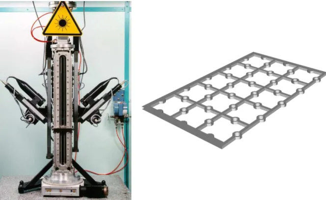
The AGATE facility was in operation from 1992 to 2001 at CEA, France (Fig. 1). The test section consists of a 5x5 rod bundle placed within a metallic channel of a square cross-section. Support grids of various designs can be inserted allowing the experimental study of the water flow, especially in the near wake of the grids. During the operating period of AGATE, more than 30 different types of mixing grids have been studied with a range of axial Reynolds number between 10,000 and 100,000. The geometry is characterized by the spatial periodicity of rods (12.6 mm), the rod-wall gap (3.1 mm) and the length of the square case (66.1 mm). The configuration considered in the present work contains two grids axially staggered and surrounding 5x3 rods and 5x2 rods (Fig. 1 and Fig. 5) respectively, and a Reynolds number of 105,000 for which a lot of experimental data are available. The upper grid is located at the height of z = 0 mm and the lower grid at the height of z = -280 mm. The grids are composed of perpendicular bars with round holes and their thickness is 1.05 mm.

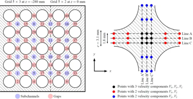
Fig. 1: The AGATE test section with the measuring devices (left) and the lower grid 5x3 (right). The non-intrusive measurement method is described by Falk and Mempontail (1998). The three components of velocity are measured at various locations (Fig. 2) by means of the laser Doppler anemometry (LDA) technique with the laser source placed on one channel side. The LDA provides the axial velocity value and one component of transverse velocity only in visible zones. Some velocity components are not reachable with a unique series of measurements. Then, two series of measurements with a rotation of the test section by 90° are required to access the velocity components at each points of Fig. 2. Moreover, the points located in the gap region are only visible alternatively by one or the other laser positioning, thus excluding the measurement of both transverse velocity

components at these locations. Finally the available velocity components in each case are listed in Table 1. The mean velocity values are averaged over 2,500 samples. Falk and Mempontail (1998) estimate the experimental uncertainty at less than 2%. The cross-section is subdivided into 16 sub-channels and 40 gaps (Fig. 2) with a numbering scheme useful for the subsequent comparisons between CFD results and experimental data.

Fig. 2: Sub-channels and gap numbering (left) and measurement locations in a sub-channel (right).

Experiment 1 Experiment 2

Black points , ,

Red points , hidden

Blue points hidden ,

Table 1: Velocity components reachable by LDA at locations shown in Fig. 2 right.

CFD analyses of experiments performed at the AGATE facility with generic PWR mixing grid was performed by Bieder et al. (2014) and Bieder et al. (2015) using RANS and LES models. In particular, they have shown that the turbulence model has a low impact on the transverse velocity and the flow patterns downstream from the mixing grid.

3. OVERVIEW OF THE TRIOCFD CODE 3.1. The CFD code TrioCFD

The code TrioCFD is based on the TRUST platform designed to manipulate equations and to provide a large range of time schemes, spatial discretizations, mathematical solvers and boundary conditions. The open-source platform TRUST is object-oriented, implemented in C++ and is designed for massively parallel computers thanks to a MPI parallelization with a quite ideal scalability up to 10,000 processor cores. In this study, TrioCFD is used for incompressible unsteady turbulent. The different models of turbulence and numerical schemes used in this study are introduced in the following sections.

3.2. Turbulence models

Three types of turbulence models are implemented in TrioCFD: Direct Numerical Simulation (DNS), Large-Eddy Simulation (LES) and Reynolds-Averaged Navier-Stokes (RANS) with − closure. For CPU time reasons, DNS remains extremely expensive to simulate full facility such as AGATE experiment. Two kinds of RANS models implemented in TrioCFD are used in this work: the standard linear − model (LEVM) and a Non-Linear Eddy-Viscosity Model (NLEVM) proposed in (Baglietto, 2006). The main differences between both − models are briefly detailed below.

We set the usual − equations:

+ = + − − ,

+ = + − − ,

=

where represents the velocity components in all corresponding directions, the viscosity, the turbulent viscosity, the density. The quantities , correspond to the turbulent kinetic energy and the turbulent dissipation rate, respectively. We have the following coefficients (Launder and Spalding (1974):

= 1.44, = 1.92, = 1.3

The difference between the two models lies in the modelling of the Reynolds stresses − : • For LEVM, the Reynolds stresses and the coefficient are given by:

− = −2₃ ,

= 0.09

• For NLEVM, quadratic terms are added in to Reynolds stresses with a modified to ensure the realizability:

− = −2₃ + −1₃ + +

+ −1₃ ,

= 2/3

+ 1₂

where = + , = − and , , depending on and are detailed in Baglietto (2006).

The LEVM performs poorly where anisotropic turbulence is the dominating mixing phenomenon. On the contrary, the non-linear extension of the Reynolds stresses allows the NLEVM to take into account the anisotropy in the flow. The NLEVM used in this work is a particular version of the non-linear eddy viscosity models family (Pope (1975), Speziale (1987), Shih et al. (1993)). This kind of non-linear models is particularly relevant to reproduce secondary flows in a square duct described by Nisizima (1990) or in a rod bundle (Baglietto, 2006) observed experimentally by Vonka (1988). According to our knowledge, the NLEVM has never been tested up to now on the type of support grid studied in this work.

LES are a major part of the TrioCFD studies. Many subgrid-scale models with various options are available. The WALE model (Wall-Adapting Local Eddy-viscosity) introduced by Nicoud (1999) is the most commonly employed model by TrioCFD users, in order to correctly calculate near-wall flows in combination with wall functions. This model has been chosen for the present LES calculation. An inlet turbulent profile computed from a preliminary periodic box calculation has been applied in the code to generate turbulence in the inflow region.

In complex industrial applications, the near-wall mesh refinement is a limiting factor for the accuracy of predictions, due to the resulting increase of the computational time. To overcome this difficulty, wall laws are employed in this study to combine insufficiently low parietal y+ values and a proper connection to the off-wall turbulent flow. Several robust methods with numerous options are available in TrioCFD to enforce the wall laws. The universal Reichardt law (Heinze, 1959) has been chosen to be conjugated with both RANS and LES models in this study.

3.3. Numerical methods and massive parallelism

In TrioCFD, the spatial discretization methods corresponding to the different types of mesh elements are called finite volume differences (FVD) for parallelepipeds and finite volume elements (FVE.) for tetrahedra (Ducros, 2010). These methods combine respectively the finite difference and the finite element methods with the finite volume method, gathering the advantages of each approach for incompressible Navier-Stokes problems. In the present study the geometry is discretized with tetrahedra using the FVE method. In this finite element method, velocity and temperature variables are located at the cell faces and the corresponding finite elements in FVE are nonconforming P1 (P1NC). The pressure is discretized in both center and the vertices of an element (P0+P1).

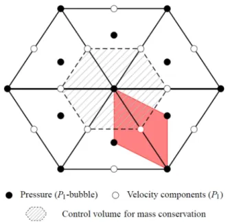
A dual mesh is built in such a way that the degrees of freedom are located at the center of dual elements, as shown on Fig. 3 in 2D, and the equations are integrated over these new control volumes. Then, the resolution in FVE is based on a variational approximation of the equations using P1 basis functions. This staggered mesh allows one to improve the velocity/pressure coupling. The resulting number of control volumes corresponds to the number of faces in the mesh, namely about twice the number of cells.

Fig. 3: Schematic 2D representation of the FVE discretization method in TrioCFD with respective positioning of degrees of freedom and control volumes.

Computations of velocity and pressure fields are decoupled using a SOLution Algorithm (SOLA) projection method, where an intermediate velocity is computed and mass conservation is then corrected by solving a Poisson equation for pressure on every control volume shown on Fig. 3. To

solve the pressure matrix inversion for RANS and LES simulations, we use PETSc2 library with the preconditioned conjugate gradient method and SSOR preconditioner.

The time integration and numerical schemes used for RANS and LES are somewhat different:

• For RANS calculations, a 2nd order centered stabilized scheme is used to discretize the convection term and a 2nd order centered scheme for the diffusion term in the momentum equation. Notice that 2nd order accuracy is necessary in TrioCFD to observe the anisotropy effects in the diffusive term with NLEVM compared to LEVM. Time integration is solved by a 1st order Euler backward implicit scheme allowing to use a multiplicative factor of time step to speed up a calculation towards the stationary state and respecting the stability. The CFL is about 10.

• For LES, the convection term is discretized by a 2nd order centered scheme stabilized scheme with a lower stabilization than in RANS simulations. A 2nd order Adams-Bashforth scheme is used for the time marching.

Data structures and functions of TrioCFD allow a simulation to be quickly parallelized and take advantage of the highest number of processor cores. For RANS and LES calculations, the whole AGATE geometry is discretized with 58 million tetrahedral cells. The generation of this mesh is described in the next section. The domain is decomposed by Metis3 in 1,800 sub-domains (32,000 cells per core) leading to a 1,800 processor cores calculation. Transfer and communication between cores use the Message Passing Interface MPI protocol. The projection method leads to solve a Poisson equation in which the pressure matrix is a sparse matrix due to the P1 nature of finite elements, of order 112 million, i.e. pressure points, in calculations presented here. The matrix is inverted by means of the PETSc conjugated gradient algorithm with SSOR preconditioning. Scalability of TrioCFD have been analyzed in a previous work with a similar HPC configuration by a strong scaling test as part of a numerical study of a nuclear assembly with mixing grids (Bieder, 2015). The AGATE calculations with both RANS models presented in this paper required a total of 80,000 CPU hours whereas 500,000 CPU hours were required for the LES calculation. All simulations have been performed on the HPC Curie supercomputer of the CEA very large computing center (TGCC).

4. NUMERICAL CALCULATIONS AND RESULTS 4.1. Calculation domain and mesh generation

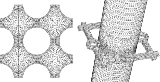
The computer-aided design was built using the SALOME platform4. The mesh was created following several steps. First, the cross-section surface was meshed by duplication of one eighth of a sub-channel, and then extruded axially creating an inlet, outlet and inter-grid domain of respectively 10, 10 and 24 hydraulic diameters of height. The gap between rods contains 13 mesh points. The two domains containing the grids were meshed separately using ANSYS ICEM CFD5 with an octree algorithm and the cross-section mesh as input. Lastly the five parts of the domain were gathered leading to 58 million of tetrahedral cells (Fig. 4). This meshing procedure provides numerous elements with perpendicular faces, which allows one to restrain the numerical diffusion. The boundary layer was meshed using two prism layers cut into tetrahedra, leading to y+ values around 35, namely in the domain of validity of standard wall functions associated with the k—ε models. The mesh resolution is suitable for LEVM and NLEVM. Moreover LES models require normally a higher mesh resolution than RANS approaches, especially in near-wall regions where boundary layer effects must be captured. However the same mesh was used for the present LES and RANS calculations, with the use of standard wall functions. According to Bieder et al. (2015), the prediction of secondary flow at the inlet is an indicator of correct meshing. Then it can be stated that the mesh refinement combined with wall 2 http://www.mcs.anl.gov/petsc 3 http://glaros.dtc.umn.edu/gkhome/metis/metis/overview 4 http://www.salome-platform.org 5 http://148.204.81.206/Ansys/150/ANSYS%20ICEM%20CFD%20Tutorial%20Manual.pdf

functions is well-adapted also for LES (see Fig. 7). Due to the computational cost, no mesh sensitivity analysis could be performed.

Fig. 4: Cross-section surface mesh around one rod (left) and rod/grid surface mesh (right). The flow at the inlet is established by means of a periodic simulation over a mesh also created by an extrusion of the cross-section. This periodic entrance domain is composed of three layers of meshes in the RANS cases and is 10 hydraulic diameters in height in the LES case in order to allow the spatial development of turbulent structures (Fig. 5). The velocity (as well as the turbulent kinetic energy and the turbulent dissipation rate in LEVM and NLEVM cases) is then imposed at the inlet of the full structure, at any instant when flow is established for LES. In the full LES simulation the velocity field is time-averaged after two crossings of the domain and over eight other crossings.

Fig. 5: Calculation domain and periodic entrance.

4.2. Convergence criteria

The LEVM and NLEVM simulations were supposed to be converged when the velocity components, turbulent kinetic energy and turbulent dissipation variations from a time step to the following were below a given threshold. Moreover it was checked that a perfect stationary state was reached in the whole domain without oscillations. The LES was supposed to be converged when the statistics, namely temporal average and standard deviation of velocity initiated from a starting time excluding

the establishment effects, were converged.

4.3. Recirculating box results

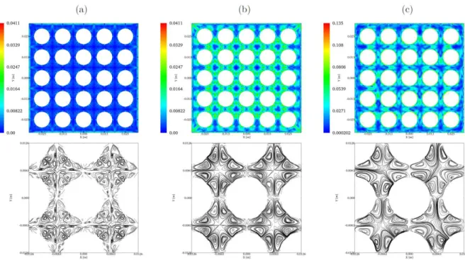
The axial and transverse velocity arising from the periodic calculations and imposed at the inlet are shown in Fig. 6 and Fig. 7. The axial velocity component is similar in each case while differences in transverse velocity magnitude are found. The LEVM provides a negligible transverse velocity compared to the two other models. Then it can be stated that this model fails at predicting the secondary flow experimentally shown by Vonka (1988) for a triangular rod arrangement. NLEVM provides an order of magnitude around 0.2% of the mean bulk velocity. This ratio is in accordance with the results found by Vonka (1988) and Baglietto and Ninokata (2005). The LES predicts higher transverse velocities than NLEVM, probably due to an incomplete flow establishment.

Fig. 6: Inlet axial velocity in m/s. (a) LEVM, (b) NLEVM, (c) LES.

Fig. 7: Inlet transverse velocity magnitude in m/s and streamlines. (a) LEVM, (b) NLEVM, (c) LES.

4.4. Axial velocity profiles

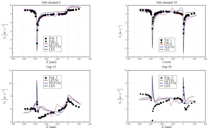
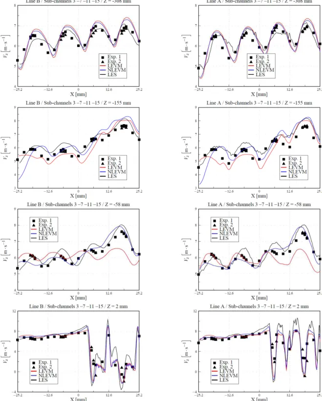
Fig. 8 and Fig. 9 show the axial velocity component plotted along vertical lines passing through sub-channels 6, 10 and gaps 19 and 30 (cf. Fig. 2) respectively, and along transverse lines A and B of

Fig. 2 at various heights. It is recalled that the entrance of the domain is located at z = -400 mm and the support grids are respectively located at the height z = -280 mm and z = 0 mm.

Fig. 8: Axial velocity along vertical lines passing through given sub-channels and gaps. The axial velocity is generally in good agreement with experimental values along the vertical lines for the three turbulence model. Discrepancies are found directly downstream from the lower grid in the gaps where all simulations overestimate the axial velocity until around 100 mm behind the grid. The velocity predicted with the LVEM is affected before the second grid, at a distance of about 100 mm upstream from this grid, whereas the NLEVM seems less impacted and the LES nearly not.

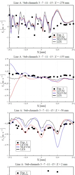
The results in transverse profiles indicate various behaviors depending on the height. Upstream from the lower grid (z = -308 mm) where the flow is controlled by advection, all three models are close together and in good accordance with experiments. The same remark remains true farther downstream (z = -155 mm) where the grid effects are dominating. Between the two grids (z = -58 mm) and far enough from the lower grid, anisotropic turbulence becomes dominating and NLEVM and LES achieve much better agreement with experiment, in comparison to LEVM. In this region the isotropy of LEVM is clearly highlighted since the axial velocity is sort of periodic. The most significant improvement of NLEVM compared to LEVM occurs in this zone. Directly after the upper grid (z = 2 mm), the inertia effects due to the grid are predominant on the anisotropic effects and no significant difference is visible between the models. These observations are in accordance with Bieder et al. (2014) and Bieder et al. (2015).

4.5. Transverse velocity profiles

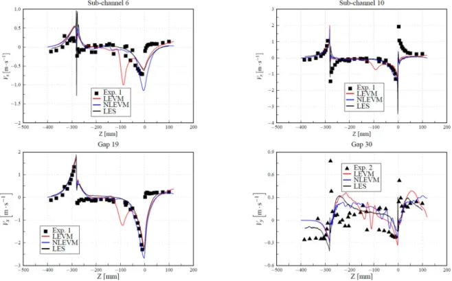
Fig. 10 and Fig. 11 present the profiles of transverse velocity along the same lines than the previous section. The vertical profiles show a good overall prediction of transverse flow even if some discrepancy is found close to the grids where the velocity gradients are strong.

Fig. 10: Transverse velocity along vertical lines passing through given sub-channels and gaps. As for the axial velocity, the transverse velocity along transverse profiles shows very little difference between the models until the lower grid, but a more substantial discrepancy with experiment. Farther downstream from the lower grid (z = -155 mm) the transverse flow is strongly overestimated close to the external wall, with an opposite direction between the LEVM and the NLEVM cases. Upstream from the upper grid (z = -58 mm) where the anisotropy effects are predominant, the LEVM provides surprisingly the best results compared to NLEVM and LES. However, it has to be highlighted that transverse velocities must be carefully interpreted due to their low order of magnitude and variation in these zones (around 1% of axial velocity). As a consequence, due to experimental uncertainties, accurate comparison between calculations and experimental measurements is tricky so that the three turbulence models can be hardly discriminated.

In general, the transverse velocity results exhibit relatively moderate agreement with experimental values, particularly in regions with strong cross-flow gradients or weak cross-flow intensity, making an accurate CFD prediction hard to achieve.

5. CONCLUSION

CFD calculations of a rod assembly with axially staggered structural grids have been performed with the TrioCFD code. Three types of turbulent models have been analyzed: the standard linear k − ε model (LEVM), a Non-Linear Eddy Viscosity Model (NLEVM) and Large Eddy Simulation (LES). The mean axial velocity calculated by both RANS approaches and LES are globally in correct agreement with experimental data. The three turbulence models provide very similar results downstream from the grids where inertia effects are dominating. However compared to the LEVM, the NLEVM and the LES achieve the best results farther from the grid where the turbulence is controlled by anisotropic effects. Contrary to the linear RANS model, the non-linear model allows one to reproduce the secondary flow also predicted by the LES approach in the region far upstream the lower grid. However, the low order of magnitude of transverse velocity far from the inlet, close to the experimental uncertainties, prevents from straightforwardly concluding about the most accurate model for correctly predicting the transverse velocity. However it can be asserted that the LES velocity provides generally the best agreement with experiment in spite of a low grid resolution and the use of wall functions.

REFERENCES

P.-E. Angeli, U. Bieder, G. Fauchet, “Overview of the TrioCFD code: main features, V&V procedures and typical applications to nuclear engineering”, Proceedings of 16th International Topical Meeting on Nuclear Reactor Thermal Hydraulics (NURETH-16), Chicago (September 2015). E. Baglietto, H. Ninokata, “A turbulence model study for simulating flow inside tight lattice rod

bundles”, Nuclear Engineering and Design, Vol. 235, pp. 773-784 (2005).

E. Baglietto, H. Ninokata, T. Misawa, “CFD and DNS methodologies development for fuel bundle simulations”, Nuclear Engineering and Design, Vol. 236, pp. 1503-1510 (2006).

U. Bieder, G. Fauchet, C. Calvin, “High performance Large Eddy Simulation of turbulent flows around PWR mixing grids“, Proceedings of 16th IEEE International Conference on High Performance Computing and Communications (HPCC 2014) – First International Workshop on HPC-CFD in Energy/Transport Domains, Paris (August 2014).

U. Bieder, F. Falk, G. Fauchet, “LES analysis of the flow in a simplified PWR assembly with mixing grid”, Progress in Nuclear Energy, Vol. 75, pp. 15-24 (2014).

U. Bieder, F. Falk, G. Fauchet, “CFD analysis of the flow in the near wake of a generic PWR mixing grid”, Annals of Nuclear Energy, Vol. 82, pp. 169-178 (2015).

F. Ducros, U. Bieder, O. Cioni, T. Fortin, B. Fournier, G. Fauchet, P. Quéméré, “Verification and validation considerations regarding the qualification of numerical schemes for LES for dilution problems”, Nuclear Engineering and Design, Vol. 240, pp. 2123–2130 (2010).

F. Falk, A. Mempontail, “Détermination d’un champ de vitesses 3D en géométrie complexe par vélocimétrie laser 2 dimensions”, 6ème congrès francophone de vélocimétrie laser, Saint-Louis, France (1998).

J.O. Hinze, Turbulence, MacGraw-Hill (1959).

B. E. Launder, D. B. Spalding, “The numerical computation of turbulent flows”, Computer Methods in

Applied Mechanics and Engineering, Vol. 3(2), pp. 269–289 (1974).

F. Nicoud and F. Ducros, “Subgrid-scale stress modelling based on the square of the velocity gradient tensor”, Flow, Turbulence and Combustion, Vol. 62, pp. 183-200 (1999).

S. Nisizima, “A numerical study if turbulent square-duct flow using an anisotropic k-eps model”,

Theoretical and computational fluid dynamics, pp. 61–71 (1990).

S. Pope, “A more general effective-viscosity hypothesis”, J. Fluid Mech., Vol. 72, pp. 331-340 (1975). T. H. Shih, Z. Jiang, J.L. Lumley, “A realizable Reynolds stress algebraic equation model”, Technical

C.G. Speziale, “On nonlinear K—l and K—ε models of turbulence”, J. Fluid Mech., Vol. 178, pp. 459-475 (1987).

V. Vonka, “Measurement of secondary flow vortices in a rod bundle”, Nuclear Engineering and