Patterns of forest vegetation responses to edge effect as revealed by a continuous approach

O

pen

A

rchive

T

OULOUSE

A

rchive

O

uverte (

OATAO

)

OATAO is an open access repository that collects the work of Toulouse researchers and

makes it freely available over the web where possible.

This is an author-deposited version published in :

http://oatao.univ-toulouse.fr/

Eprints ID : 16278

To link to this article : DOI :10.1007/s13595-013-0301-0

URL :

http://dx.doi.org/10.1007/s13595-013-0301-0

To cite this version : Alignier, Audrey and Deconchat, Marc Patterns

of forest vegetation responses to edge effect as revealed by a

continuous approach. (2013) Annals of Forest Science, vol. 70 (n° 6).

pp. 601-609. ISSN 1286-4560

Any correspondance concerning this service should be sent to the repository

Patterns of forest vegetation responses to edge effect

as revealed by a continuous approach

Audrey Alignier&Marc Deconchat

Abstract

&ContextUnderstanding the variability of vegetation distri-bution and its determinants is a central issue for addressing the effects of edges on ecological processes. Recent studies have revealed inconsistencies in the patterns of responses to edge effects that raise important questions about their deter-minants. We investigated the edge effect response patterns by adapting a recently proposed continuous approach to the case of small forest fragments in southwestern France. &Methods We surveyed forest understory vegetation (com-position, species richness, and percent cover) and abiotic variables (soil temperature, moisture, pH, and canopy open-ness) along 28 transects across hard forest edges. We tested five statistical models to describe the response pattern of each variable (1) over all transects and (2) per transect. We then compared the response patterns as a function of the attributes of the edge (orientation, topography, and adjacent land cover) and forest patch size.

&Results Over all transects, a general decreasing trend was observed for all variables as the distance from the edge increased. In the individual transects, we evidenced a large variability in the response patterns that was not related to edge attributes or to patch size.

& Conclusion It is difficult to assess the depth of edge influence in highly fragmented forests and to identify the determinants of edge effects. We recommend that care should be taken with studies using pool of transects, and that further studies should be carried out including situations with neutral patterns, in order to gain a broader understand-ing of edge effects on vegetation.

Keywords Understory vegetation . Edge effect . Forest edge . Neutral response . Logistic model

1 Introduction

Forest edges are ubiquitous elements of fragmented forests in many temperate landscapes, where they influence biodi-versity distribution. These discontinuities between forest and a more open habitat induce a transition zone on both sides of the border, called the edge effect (Murcia 1995). Among factors associated with forest fragmentation, edge effects have been reported as one of the most significant patterns structuring both flora and environmental conditions (Ewers and Didham2006a; Ewers and Didham2008). For example, gradual changes from the border towards the forest interior have been identified for air humidity (Kapos1989), soil moisture (Jose et al. 1996), air and soil temperature (Williams-Linera 1990), and solar radiation (Brothers and Spingarn1992). Diversity, composition, dynamics, and spa-tial distribution of plant communities going into the forest are also largely shaped by the response of species to edge influence (Harper et al.2005). Variations of edge effects on vegetation distribution in forest fragments need to be more clearly understood, so they can be integrated in the manage-ment of biodiversity in fragmanage-mented forests.

A challenge for understanding edge effects emerges from the inconsistency of the observed patterns. Edge effects are sensitive to several contextual factors including matrix type,

A. Alignier

:

INRA, UMR 1201 DYNAFOR, 31326 Castanet Tolosan, France A. Alignier (*)

:

Université de Toulouse, ENSAT; UMR 1201 DYNAFOR, 31326 Castanet Tolosan, France

edge orientation, edge contrast, topography, time since distur-bance, patch size, and shape (Honnay et al.2002; Gonzalez et al.2010; Chabrerie et al.2013; Pellissier et al.2013). While results from empiric studies confirm that many species re-spond to edge effects, some authors have put forward the idea that a neutral response to edge effects could be more frequent than previously thought (Ries and Sisk2010).

Many empirical and theoretical studies have looked for a standardized tool for describing and quantifying edge effects. In a previous work, we identified the lack of a common pattern capable of properly defining edge influence on vegetation. We showed that a discrete approach, with reference to the hypothetical two-phase response pattern proposed by Murcia (1995), failed adequately to quantify the depth of edge influence (DEI) (Alignier and Deconchat

2011). To better understand the ecological processes that operate in relation to the presence of an edge, it is more important to focus on the edge influence response patterns than to quantify depth of edge influence. A better statistical approach, exploring a larger set of possible continuous models (Ewers and Didham2006b), is required to confirm these results.

We investigated the determinants of variation in the edge effect response patterns in small fragmented forests. We addressed the following two questions: (1) how do the forest understory vegetation (composition, species richness, and percent cover) and environmental conditions (soil tempera-ture, soil moistempera-ture, soil pH, and canopy openness) vary with the distance from the border? And (2) how do these re-sponse patterns vary with the edge attributes (edge orienta-tion, topography, and adjacent land cover) and forest patch size? We adapted the continuous approach proposed by Ewers and Didham (2006b) for describing response patterns of biotic and abiotic data to edge effects. This work goes further than earlier studies by using a continuous approach to document the edge influence response patterns in frag-mented forests, by integrating several edge attributes, and using a larger sample of edge transects than in most similar works (e.g., Gehlhausen et al. 2000; Ewers and Didham

2008).

2 Material and methods 2.1 Study area

Field work was conducted in the district of Aurignac (43°13′ N 0°52′E) in the Vallées et Coteaux de Gascogne area, a long-term ecological and socioeconomic study site (LTER-Europe,

www.lter-europe.net) in southwestern France. The climate is temperate with oceanic and Mediterranean influences. The summers are quite hot and dry and the winters mild and damp with an average annual temperature of 11 °C and annual

rainfall of 750 mm. The hillsides are modeled in the Molasse, a detrital argilo-calcareous formation. The forests are frag-mented with patch size between 0.5 and 35 ha and cover approximately 15 % of the study area. Most of these forest fragments have been isolated since the beginning of the nineteenth century, and their contours have remained un-changed, or nearly so, since the first aerial photographs were taken in 1942. The main tree species are Quercus robur and Quercus pubescens, Carpinus betulus, Prunus avium, and Sorbus torminalis. The management system is coppice-based, with trees intended for industrial purposes. The woods are privately owned and managed.

2.2 Sampling design

Variations in the understory vegetation composition were examined along a set of 28 transects belonging to hard edges (i.e., edges showing high contrast with the adjacent matrix) in direct contact with adjacent land cover. These transects have already been used by Alignier and Deconchat (2011). Edges bordering on roads, tracks, or streams were excluded. Transects pertained to seven mature woodlots chosen be-cause of their shared history: two centuries ago, they were all part of the same native forest (Andrieu et al.2011). They therefore presented relative homogeneity in canopy compo-sition, age, and structure. Forest patch size averaged 11.5 ha and varied from 3.4 to 42.7 ha. Hard edges were selected according to two adjacent land cover classes (crop and meadow), two orientation classes (north and south), and two topographical position classes (ascending and neutral). Ascending position means the transect orientation from the forest interior towards the border is upslope. Neutral posi-tion means the transect is neither upslope nor downslope. Each combination of adjacent land cover, orientation, and topography (n=8), except for the crop-north-upslope com-bination, which is not encountered in the study area, was replicated four times yielding a total of 28 transects.

Transects extended perpendicularly from the border (0 m), defined as the line formed by trees with a diameter of more than 10 cm at chest height, towards the forest interior for a distance not exceeding 40 m. We focused on the forest side only. The limitation stressed by some recent works, whereby certain studies have only considered the “one-sided” portion of the edge response from the patch edge to the patch interior and ignored the “two-sided” nature of edge effects (Fonseca and Joner 2007), was considered irrelevant in our case because the agricultural patches are dominated by intensively managed crops and are more highly disturbed than the forest habitat. Such human-dominated areas inhibit the natural dynamic of the flora. Moreover, Ewers and Didham (2006b) acknowledge that when the values of a given variable are obviously and trivially equal to zero (e.g., tree density in a grassland–forest

boundary), the inclusion or exclusion of these zeros makes little difference. We consider that this is the case for most of our variables, except for soil conditions.

Because a length of 40 m reached the center of certain forest fragments, we considered it irrelevant to sample lon-ger transects. To limit multiple edge effects, transects were situated at least 40 m from a canopy opening or from any other edge. Transects were at least 40 m apart and were relatively homogeneous, without any intersections with farm tracks or gaps. Twenty contiguous 2 by 2 m quadrats were established along each transect.

2.3 Vegetation data

Understory vegetation was sampled in each quadrat from May to the end of June 2008, allowing us to take into account the vernal flora. The percent cover for all the vascular species was estimated visually using a reference grid (Prodon and Lebreton1981). Individuals with a diam-eter of more than 1 cm at a height of 2 m, mainly consisting of mature individuals of woody species, were excluded from the analysis. Their presence in the forest fragments results more from management practices than from the ecological conditions associated with the edges (McCollin et al.2000). The plant nomenclature follows Flora Europaea (Tutin et al.

1993). The following variables were derived from the flo-ristic data: species composition, species richness, and per-cent cover.

To reduce species composition data to a few interpretable variables, we used linear ordinations (e.g., Gehlhausen et al.

2000). First, we conducted a single principal component analysis on the variance/covariance matrix (covPCA) of all the vegetation transects. Only the scores on the first axis were kept to summarize the composition of each quadrat owing to the largest part of explained inertia. Second, we performed 28 independent covPCAs to address the varia-tions in the species composition for each transect.

2.4 Environmental data

Soil temperature, moisture, pH, and canopy openness were measured on the same quadrats as for the vegetation data. They are known to influence vegetation distribution and to be potentially influenced by edge effect (Chen et al.1992; Jose et al.1996). All these variables were measured at the beginning of summer, with the exception of the percentage of canopy openness, which was measured at the end of July, when the vegetation of the overstorey canopy was fully developed. All data were collected during the same short period to limit the influence of weather conditions.

Soil temperature was measured 10 cm below the soil sur-face using a portable temperature probe (Hanna HI935005N). Simultaneously, relative soil moisture was measured 5 cm

below the surface of the litter-free forest soil (ThetaProbe hygrometer, Delta-T Device Ltd). Soil samples, taken at a depth of 10 cm, were collected in hermetically sealed bags and brought back to the laboratory. Soil pH was measured by putting the soil in a solution of distilled water in the proportion 1:1. The measurements were repeated five times for each variable and each quadrat to take into account the very fine scale variability. Canopy openness was estimated from hemi-spherical photographs of the forest canopy taken with a Nikon Coolpix 4500 digital camera, with a fisheye lens (Nikon FC-E8). The photographs were taken every 8 m, along each transect, starting from the center of the first plot. The percent-age of canopy openness was calculated from the photographs with the Gap Light Analyser 2.0 software. Interpolated values between these measurements were assigned to each quadrat along the transect.

2.5 Statistical analyses

In line with Ewers and Didham (2006b), we fitted five statistical models to explore the response of the understory vegetation and environmental conditions to edge effect:

Null model v¼ v þ ε ð1Þ Linear model v¼ β0þ β1dþ ε ð2Þ Exponential model v¼ β0eβ1dþ β2þ ε ð3Þ Logistic model v¼ β0þ β₁−β0 1þ eðβ2−dÞβ3þ ε ð4Þ Unimodal model v¼ β0þ β1−β0 1þ eðβ2−dþβ4d2Þβ3 þ ε ð5Þ where v is the response variable, d the distance from the border, β0, β1, β2, β3regression coefficients, and ε the error

term. These models do not necessarily represent the best fit to the data, but they do have the advantage of referring to ecological hypotheses, empirically demonstrated, on the response of communities and environment to edge influence.

We used the information–theoretical approach as model selection procedure. To compare the five statistical models in an unbiased way, we used Akaike information criterion weights (calculated from Akaike information criterion (AIC) values). Akaike weights are normalized across the set of candidate models to sum to one, and give the proba-bility that a particular model is the best fit to the data from

the set of candidate models (Johnson and Omland 2004). Like Ewers and Didham (2008), we added an additional constraint for selecting the unimodal model. To ensure that the unimodal model was selected only in the case where there was a clear unimodal peak, we compared the values of the extremes of the gradient with the maximum value on the fitted curve. If the extreme values represent less than one third of the peak value, then the peak is considered to be significant and the unimodal model val-idated. Otherwise, the unimodal model was discarded in favor of the model with the next lowest AIC weight. We used the second derivatives of the logistic and unimodal models to calculate the depth of edge influence, i.e., DEI (Eqs. 4 and5; see Ewers and Didham (2006b) for further details).

First, we addressed the pattern of the responses of both the biotic and abiotic variables to edge effect, pooling data over all transects. For each variable, we tested five mixed effect models derived from the five statistical models of Ewers and Didham (2006b). Fixed terms consisted of dis-tance from the border, edge orientation, topography, adja-cent land cover, and forest patch size (Online Resource1). We only considered fixed terms in an additive way and excluded interactions due to their relatively large number (n=10) by comparison with the dataset size (n=28 for each variable). Transect identity (n=28) was included as random terms. R2for mixed effect models were calculated according to Nakagawa and Schielzeth (2013).

In a second step, transects were assumed to be indepen-dent. The edge influence response patterns for each variable and each transect were examined using the same five statis-tical models as Ewers and Didham (2006b). We then com-pared the proportion of each statistical model selected by the largest AIC weight as a function of edge attributes, using chi-square tests. Thirdly, we quantified DEI for each vari-able and each transect. As we encountered few logistic and unimodal models (n=28 for all variables; Online Resource

2), we chose to use all the cases, where these models were significant, even if they were not selected (n=38) as best models by AIC weights to determine DEI. We addressed the effect of edge attributes and forest patch size on (1) the parameter associated with distance-to-edge in linear models and (2) on all DEI using linear mixed effect models (LMMs), adding transect nested in woodlot as random terms. We considered DEI over all variables to increase the statistical power of analysis (Online Resource1). Final-ly, we determined whether DEI per variable varied with edge attributes (Wilcoxon rank tests) or forest patch size (Spearman rank correlation tests). We excluded the use of LMMs due to the small number of DEIs per variable. All analyses were performed using R 2.12.0 (R Development Core Team 2008), with the nlme package (Pinheiro et al.

2012).

3 Results

3.1 Vegetation and environmental data

We identified 127 plant species with 10.7±3.6 (mean ± SE) species on average per quadrat and 32.7±8.7 species on average per transect; 45 species were woody, and only 5 species were annuals (Conyza sumatrensis, Galium aparine, Poa annua, Stellaria media, and Veronica hederifolia). The species most often found along the transects were Hedera helix, Rubus fructicosus gr., Tamus communis, Lonicera periclymenum, P. avium, and Rubia peregrina, with a fre-quency higher than 50 %, representing less than 5 % of the plant species identified. A large majority (80 %) of the species were relatively uncommon, with a frequency lower than 10 % over all transects. Plant cover per quadrat was 50.4±27.4 % on average. The first two axes of the global covPCA explained 54.8 % of the variance, with individual axes explaining 35.4 and 19.4 %, respectively. The total inertia of the 28 single covPCAs was 4.22±1.23 on average. The eigenvalues of the first axes of the 28 covPCAs vary between 0.48 and 1.69, with a mean of 0.93. The part of variance explained by the first axis was 22.2±4.9 % on average.

The average soil temperature and moisture measured over all the quadrats were 17.9±0.8 °C and 12.2±3.4 %, respectively. Soil pH varied between 4.4 and 7.2 and aver-aged 5.4±0.4. Lastly, the percentage of canopy openness averaged 19.5±4.3 %.

3.2 Overall edge effect response patterns

Among the variables, the null model was selected as the best model for species richness only. Percent cover decreased linearly, as the distance from the border increased, whereas soil temperature and moisture increased linearly (Fig. 1; Online Resource 1). The exponential model was selected as the best model for pH and canopy openness, with a decrease in values as the distance from the border increased. Only the scores on the first axis of the global covPCA were fit best by a logistic model (Fig.1). On the whole, orienta-tion, topography, adjacent land cover, and forest patch size had no significant relationship with biotic or abiotic varia-bles (Online Resource1).

3.3 Edge effect response patterns per transect

For biotic variables, each of the five statistical models was selected at least once as the best model except for percent cover, for which the unimodal model was never chosen (Table 1; Online Resource 2). For abiotic variables, the logistic and unimodal models were never selected for soil pH and canopy openness. Out of all the variables, we

noticed that the null model was most often selected as the best model. The logistic model was the most frequent best model for vegetation composition only, and the linear model was the most frequent best model for soil temperature only (Table 1). Overall, biotic and abiotic variables tended to decrease as the distance from the border increased, except for soil temperature and soil moisture (Table1).

3.4 Edge attribute relationship to response patterns

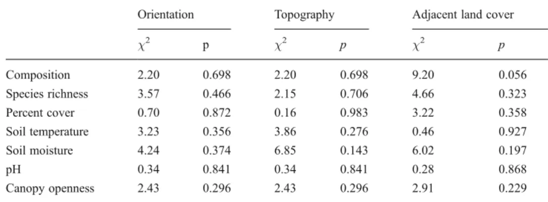
The proportion of the different models selected by the AIC weights for each variable did not vary significantly accord-ing to forest edge attributes (Table2).

3.5 Edge attribute relationship to slopes and DEI

Considering only linear models selected as best models by AIC weights, the parameters associated with distance-to-edge (i.e., slopes) were not significantly related to distance-to-edge attributes and forest patch size (Table3a).

For all variables, edge effects penetrated by about 18.5± 5.4 m in north edges versus 18.5±6.5 m in south edges. DEIs were 19.2±5.9 m in ascending edges versus 18.2± 6.1 m in neutral edges and 19.30±4.4 m in forest edges facing crops versus 17.8±7.8 m in forest edges facing meadows. DEIs were not related to edge attributes and forest patch size (Table 3b). Considering DEIs for each

Fig. 1 Best model selected for each biotic and abiotic variable overall transects (n=28). Models consisted in nonlinear mixed effects models with distance from the border, edge orientation, topography, adjacent land cover, and forest patch size as fixed terms and transect identity as random term

variable (Table4), we did not find any significant difference according to edge attributes or forest patch size (Table5).

4 Discussion

Using the continuous approach proposed by Ewers and Didham (2006b), we identified different patterns of responses to hard edges in forest understory vegetation and related environmental conditions. These patterns seem to depend on the spatial extent considered. On all transects, we observed a general trend towards a decrease in the variables, as the distance from the border increased. On a finer scale, a large part of the variables tested exhibited response patterns best fitted with null models. Contrary to expectations, we were not able to determine depth of edge influence in small forest fragments, and the determinants of variation in edge effects in highly fragmented forests remain unclear. These results combine to underline the value of investigating edge effects in highly fragmented forests for understanding better their impact on biodiversity.

Out of all the data, forest edges significantly influenced vegetation and environmental conditions. The linear model was often selected as the best fit to data. According to the literature, the structure and diversity of the communities are characteristically altered at habitat edges (Ewers and Did-ham2006b; Gehlhausen et al.2000). Plant species richness and percent cover are known to decrease, as distance increases from the border towards the forest interior (Brothers and Spingarn1992). In our case, species richness was constant (i.e., fitted by null model), whereas species composition changed up to a distance of 18 m. Plant com-munities were as rich near edges as towards the forest interior, but plant assemblages were different. This change in species composition may reflect the functional response of species. Indeed, forest habitat specialists are generally shade-tolerant and are known to avoid edges (Ranney et al.

1981). In addition, light availability is generally greater near forest edges advantaging light-tolerant species near the bor-der (Brothers and Spingarn 1992). However, we failed to detect similar trends in the main vegetation composition and canopy openness response patterns. Earlier studies have shown that soil moisture is lower near the edge than in the forest interior in relation to greater luminosity, higher air and soil temperatures, and lower air humidity at soil level (Kapos1989; Jose et al.1996). Here, soil temperature and moisture increased linearly along the transect towards the forest interior, whereas pH and canopy openness exhibited decreasing exponential patterns as the distance from the border increased. The edge might play the role of filter with respect to pollutants generated by human activities in the adjacent habitats (Weathers et al.2001), hence a higher pH at the edge. In contrast, the soil temperature pattern is more

T able 1 Number of best models selected by AIC weights for each variable. The mean R 2(min – max) and mean AIC (min – max) was given for each statistical model. In bold, the maximum number of selected model amongst the five statistical models tested. In brackets, the number of negative edge ef fects according to regression coeffi cients (sensu Ries et al. 2004 for logistic models) Nul l AIC Lin . R 2 A IC Exp. R 2 AIC Log. R 2 AIC Uni . R 2 AIC Composit ion 3 58.81 (55.31 – 65.01 ) 7 (7) 0.45 (0.22 – 0.74) 48.77 (35.09 – 69.33 ) 7 0.58 (0.25 – 0.84) 36.57 (27.05 – 54.54 ) 9 (0) 0.79 (0.40 – 0.95) 31.89 (10 – 85 – 59.64) 2 0 .8 1 (0 .7 4– 0 .8 8 ) 33.67 (33 .37 – 33.97 ) Richne ss 15 52.09 (43.91 – 64.28 ) 7 (5) 0.28 (0.1 1– 0.56) 100.8 9 (77.78 – 1 15.28 ) 1 0.33 102.66 3 (2) 0.47 (0.31 – 0.64) 1 0 0 .8 9 (2 1 8 .7 9– 2 2 3 .5 3 ) 2 0 .8 1 (0 .7 8– 0 .8 3 ) 92.98 (92 .09 – 93.88 ) Percent cover 17 2 2 7 .5 0 (1 9 9 .0 6– 2 4 1 .2 2 ) 4 (1) 0.31 (0.13 – 0.53) 181.8 7 (170.87 – 196.8 3) 2 0.52 (0.28 – 0.75) 155.77 (152.31 – 15 9.23) 5 (1) 0.58 (0.36 – 0.92) 1 6 1 .1 9 (1 3 3 .6 6– 1 8 6 .0 1 ) 0 – – T em perature 6 − 3.81 (− 22.32 – 1.83) 13 (3) 0.39 (0.09 – 0.72) − 14.53 (− 33.29 – 1.24) 6 0.67 (0.55 – 0.92) − 19.96 (− 33.9 – 0.47) 3 (3) 0.83 (0.76 – 0.92) − 1 8 .9 3 [− 2 0 .4 7– (− 1 5 .9 7 )] 0 – – Moist ure 16 76.14 (63.68 – 88.57 ) 7 (3) 0.29 (0.12 – 0.48) 92.92 (71.79 – 1 12.08 ) 1 0.46 78.54 1 (1) 0.87 77.55 3 0 .7 5 (0 .6 8– 0 .8 7 ) 67.1 1 (46.91 – 84.1) pH 1 1 1 1.94 (− 25.35 – 83.16) 1 1 (8) 0.32 (0.12 – 0.60) 7.91 (− 14.13 – 26.37 ) 6 0.58 (0.20 – 0.89) − 5.75 (− 16.04 – 7.78) 0 – – 0 – – Canopy open. 14 52.09 (43.91 – 64.28 ) 8 (8) 0.43 (0.23 – 0.85) 53.01 (44.37 – 69.33 ) 6 0.79 (0.54 – 0.95) 44.25 (35.81 – 51.9) 0 – – 0 – –

difficult to interpret and depends strongly on season and time of day. The forest interior is generally thought to buffer climatic fluctuations, but we cannot test this assumption here, as we measured soil temperature only once.

Addressing the edge effect response patterns per variable and per transect, we showed a great variability among biotic and abiotic data. Each of the five statistical models was select-ed at least once to describe variations in response to select-edge effect. This result corroborated our previous observations of discrep-ancies between vegetation response patterns and the hypothet-ical response pattern (Alignier and Deconchat2011). Given the great dispersion of the data leading to a great variability in the edge influence response patterns among variables and trans-ects, we recommend that care should be taken with edge effect studies using pool of transects (e. g., Chen et al.1992).

The most striking result was the preponderance of null and linear models selected to describe both vegetation and envi-ronmental response patterns. Despite our efforts to limit con-founding factors, i.e., edge aspect, this result contrasts with the literature on forest edges usually demonstrating positive or negative effects on biotic and abiotic factors (Harper et al.

2005). Our study was conducted in small fragmented forests, with an area of between 5 and 45 ha. We hypothesize that the

size of our forest patches was too small to guarantee the presence of a core habitat zone. In that sense, forest patches can be considered to be entirely under the influence of the edge (Laurance and Yensen1991) or of multiple edge effects (Fletcher 2005). Under these conditions, it can be assumed that the patterns of biodiversity response to edges in a highly fragmented context no longer obey the general trends ob-served in larger woods.

Conversely, we cannot exclude stochastic events induced by the fine scale of observation (i.e., spatial resolution). The weak relationship between habitat selection and habitat quality may result from the influence of nonvegetation habitat features (e.g., climatic fluctuations), nonequilibrium conditions, and the influence of stochastic variation, which are preponderant on small spatial and temporal scales (Campbell et al.2010). Stochasticity is rarely investigated explicitly as a determinant of habitat use patterns. Stochastic events may challenge the primacy of deterministic explanations, i.e., edge effect.

Contrary to our expectations, neither forest edge attrib-utes (orientation, topography, and adjacent land cover) nor did forest patch size significantly explain the observed var-iability in response patterns. Although our forest fragments pertained to the same native forest and were thus considered

Table 2 Summary of the chi-squared tests testing the effect of forest edge attributes on the number of the five statistical models selected for each variable

Orientation Topography Adjacent land cover χ2 p χ2 p χ2 p Composition 2.20 0.698 2.20 0.698 9.20 0.056 Species richness 3.57 0.466 2.15 0.706 4.66 0.323 Percent cover 0.70 0.872 0.16 0.983 3.22 0.358 Soil temperature 3.23 0.356 3.86 0.276 0.46 0.927 Soil moisture 4.24 0.374 6.85 0.143 6.02 0.197 pH 0.34 0.841 0.34 0.841 0.28 0.868 Canopy openness 2.43 0.296 2.43 0.296 2.91 0.229

Table 3 Summary of the linear mixed effect model (LMM) to analyze effects of edge attributes (orientation, topography, and adjacent land cover) and forest patch size on (a) the parameter of linear models

associated to distance-to-edge (i.e., slope) and (b) DEI overall variables and transects. Random terms consisted in transect nested in woodlot. F and p value (p) from ANOVA type III error tests are given

Value SE F value p

(a) Slope of linear models

Orientation (south) −0.12 0.12 0.05 0.223 Topography (neutral) −0.13 0.09 0.36 0.165 Adjacent land cover (meadow) −0.08 0.09 0.67 0.358

Woodlot area −0.002 0.002 0.35 0.299

b) DEI over all variables

Orientation (south) 19.73 2.37 0.05 0.828 Topography (neutral) −1.37 2.30 0.36 0.560 Adjacent land cover (meadow) −1.89 2.30 0.67 0.427

as equally suitable habitat, they may differ as a result of their recent management history. Brosofske et al. (2001) showed that the effect of disturbances may override the edge effects. The lack of consistency between our vegetation patterns and the hypothetical response pattern may correspond to a situ-ation where the distinction between plant communities near edges and towards the forest interior has not yet been made. Studies reported that vegetation may react with a delay to the recent creation of a discontinuity or disturbance, i.e., some species are still temporarily present even though the conditions favorable to their survival have disappeared (Vellend et al. 2006). However, this hypothesis is more debatable in the case of abiotic variables, which are assumed to be more reactive to recent disturbances.

Information on effective edge extent is critical for imple-menting different management measures on forest edges with a view to controlling their effects on the adjacent land cover and to maintaining biodiversity in the forest interior. Only a few responses fitted by logistic and unimodal models were found. The drawback of this result is that we cannot rigorously quantify the extent of edge effects in our study area or provide robust conclusions. As previously shown

(Alignier and Deconchat2011), it seems better to perform detailed analysis of edge response patterns in order to in-vestigate edge effects, rather than to quantify depth of edge influence.

With this study, we have evidenced a great variability in the vegetation and environmental data patterns in response to the edge influence, and shown that depth of edge influence cannot be well-defined in small forest fragments. With this work, we have moved beyond our earlier study (Alignier and Deconchat 2011), as we have analyzed the response patterns by characterizing the edge influence re-sponse patterns using a continuous approach; it has also provided empirical explanations, in most cases, for the dis-crepancies found with respect to the hypothetical patterns for both vegetation and environmental conditions. Our study is one of the few to have purposefully distinguished between confounding factors (such as edge attributes and forest patch size) to address the edge influence response patterns. With a view to managing biodiversity in the edge and assessing the influence that it may have on adjacent environments, par-ticularly through ecological services, studies are still re-quired in order to detail the relevant factors and mechanisms

Table 4 Mean ± SE depth of edge influence (DEI) for each variable according to forest edge attributes. DEI was obtained from second derivatives of logistic and unimodal models, even if they were not selected as best models

Orientation Topography Adjacent land cover

North (N=12) n South (N=16) n Upslope (N=12) n Neutral (N=12) n Crop (N=12) n Meadow (N=16) n Composition 22.3±6.4 6 16.0±8.0 8 17.2±5.4 5 19.5±9.1 9 18.3±4.7 7 19.1±10.5 7 Species richness 17.5±2.1 2 18.3±2.9 4 22.5±7.8 2 15.8±2.9 4 19.2±5.1 5 12* 1 Percent cover 14.0±1.4 2 18.2±2.9 5 15.0±0 2 17.8±3.6 5 18.2±3.4 4 15.3±2.5 3 Soil temperature 13.0±1.4 2 21.3±7.5 3 25.0±5.6 2 13.3±1.5 3 17.5±4.9 2 18.3±9.3 3 Soil moisture 18.5±2.1 2 20.5±3.5 2 – 0 19.5±2.6 4 19.3±3.2 3 20 * 1 pH 17.0* 1 – 0 – 0 17* 1 – 0 17* 1 Canopy openness – 0 28* 1 – 0 28* 1 28* 1 – 0 The number of DEI obtained (n) is mentioned in brackets. Asterisk indicates that SD cannot be computed because there is only one value of DEI

Table 5 Effects of forest edge attributes on the mean depth of edge influence for each variable. Results are for Wilcoxon rank tests (W) for edge attributes and Spearman correlation tests (rho) for forest patch

size. Tests were performed with DEI from logistic and unimodal models, even if they were not selected as best models by AIC weights

Orientation Topography Adjacent land cover Forest patch size

W p W p W p rho p Composition 35.5 0.155 18.5 0.640 19.0 0.522 0.12 0.662 Species richness 4.5 1.000 7.0 0.240 5.0 0.234 0.22 0.676 Percent cover 0.5 0.114 2.0 0.324 9.0 0.368 0.27 0.552 Soil temperature 0.5 0.236 6.0 0.138 3.5 1.000 −0.57 0.312 Soil moisture 1.0 0.667 – – 1.0 1.000 −0.45 0.552 pH – – – – – – – – Canopy openness – – – – – – – –

lying behind the response patterns of biotic and abiotic data in highly fragmented forests.

Acknowledgments We thank Laurent Burnel, Jérôme Willm, and Marc Fakorellis for their assistance in the field. We are also grateful to Alain Cabanettes and Michel Goulard for providing comments on statistical analysis. We thank Huw ap Thomas (Axtrad) for thorough editorial advice in English. We thank the three anonymous reviewers for their constructive comments. Funding for this study was provided by the French Ministry of Research and Education.

References

Alignier A, Deconchat M (2011) Variability of edge effect on vegeta-tion implies reconsideravegeta-tion of its assumed hypothetical pattern. Appl Veg Sci 14:67–74

Andrieu E, Ladet S, Heintz W, Deconchat M (2011) History and spatial complexity of deforestation and logging in small private forests. Landsc Urban Plan 103:109–117

Brosofske KD, Chen J, Crow TR (2001) Understory vegetation and site factors: implications for a managed Wisconsin landscape. For Ecol Manage 146:75–87

Brothers TS, Spingarn A (1992) Forest fragmentation and alien plant invasion of Central Indiana old-growth forests. Conserv Biol 6:91–100 Campbell SP, Witham JW, Hunter ML Jr (2010) Stochasticity as an alternative to deterministic explanations for patterns of habitat use by birds. Ecol Monog 80:287–302

Chabrerie O, Jamoneau A, Gallet-Moron E, Decocq G (2013) Matu-ration of forest edges is constrained by neighboring agricultural land management. J Veg Sci 24:58–69

Chen JQ, Franklin JF, Spies TA (1992) Vegetation responses to edge environments in old-growth Douglas-fir forests. Ecol Appl 2:387–396 Ewers RM, Didham RK (2006a) Confounding factors in the detection of species responses to habitat fragmentation. Biol Rev 81:117–142 Ewers RM, Didham RK (2006b) Continuous response functions for

quantifying the strength of edge effects. J Appl Ecol 43:527–536 Ewers RM, Didham RK (2008) Pervasive impact of large-scale edge effects on a beetle community. Proc Natl Acad Sci 105:5426–5429 Fletcher RJ (2005) Multiple edge effects and their implications in

fragmented landscapes. J Anim Ecol 74:342–352

Fonseca CR, Joner F (2007) Two-sided edge effect studies and the restoration of endangered ecosystems. Restor Ecol 15:613–619 Gehlhausen SM, Schwartz MW, Augspurger CK (2000) Vegetation

and microclimatic edge effects in two mixed-mesophytic forest fragments. Plant Ecol 147:21–35

Gonzalez M, Ladet S, Deconchat M, Cabanettes A, Alard D, Balent G (2010) Relative contribution of edge and interior zones to patch size effect on species richness: an example for woody plants. For Ecol Manage 259:266–274

Harper KA, Macdonald SE, Burton PJ, Chen JQ, Brosofske KD, Saunders SC, Euskirchen ES, Roberts D, Jaiteh MS, Esseen PA (2005) Edge influence on forest structure and composition in fragmented landscapes. Conserv Biol 19:768–782

Honnay O, Verheyen K, Hermy H (2002) Permeability of ancient forest edges for weedy plant species invasion. For Ecol Manage 161:109–122

Johnson JB, Omland KS (2004) Model selection in ecology and evolution. Trends Ecol Evol 19:101–108

Jose S, Gillespie AR, George SJ, Kumar BM (1996) Vegetation responses along edge-to-interior gradients in a high altitude tropical forest in peninsular India. For Ecol Manage 87:51– 62

Kapos V (1989) Effects of isolation on the water status of forest patches in the Brazilian Amazon. J Trop Ecol 5:173–185 Laurance WF, Yensen E (1991) Predicting the impacts of edge effects

in fragmented habitats. Biol Conserv 55:77–92

McCollin D, Jackson JI, Bunce RGH, Barr CJ, Stuart R (2000) Hedgerows as habitat for woodland plants. J Environ Manage 60:77–90

Murcia C (1995) Edge effects in fragmented forests: implications for conservation. Trends Ecol Evol 10:58–62

Nakagawa S, Schielzth H (2013) A general and simple method for obtaining R2from generalized linear mixed effects models. Meth-ods Ecol Evol 4:133–142

Pellissier V, Bergès L, Nedeltcheva T, Schmitt M-C, Avon C, Cluzeau C, Dupouey J-L (2013) Understory plant species show long-range spatial patterns in forest patches according to distance-to-edge. J Veg Sci 24:9–24

Pinheiro J, Bates D, DebRoy S, Sarkar J and the R Development Core Team (2012) nlme: linear and nonlinear mixed effects models. R package version 3.1-104.

Prodon R, Lebreton J-D (1981) Breeding avifauna of a Mediterranean succession: The Holm oak and cork oak series in the eastern Pyrenees, 1. Analysis and modeling of the structure gradient. Oikos 37:21–38

R Development Core Team (2008) R: A language and environment for statistical computing. Vienna, Austria

Ranney JW, Bruner MC, Levenson JB (1981) The importance of edge in the structure and dynamics of forest islands. In: Burgess R.L. and Sharpe D.M. (Eds), Forest island dynamics in man-dominated landscapes, Springer Verlag, pp. 67–95.

Ries L, Fletcher Jr RJ, Battin J, Sisk TD (2004). Ecological responses to habitat edges: mechanisms, models, and variability explained. Ann Rev Ecol Evol Syst 35:491–522

Ries L, Sisk TD (2010) What is an edge species? The implication of edge sensitivity to habitat edges. Oikos 119:1636–1642 Tutin TG, Burges NA, Chater AO, Edmondson JR, Heywood VH,

Moore DM, Valentine DH, Walters SM, Webb DA (1993) Flora europaea, Cambridge Univ. Press, 581 p

Vellend M, Verheyen K, Jacquemyn H, Kolb A, Van Calster H, Peterken G, Hermy M (2006) Extinction debt for forest plants persists for more than a century following habitat fragmentation. Ecology 87:542–548

Weathers KC, Cadenasso ML, Pickett STA (2001) Forest edges as nutrient and pollutant concentrators: potential synergisms be-tween fragmentation, forest canopies, and the atmosphere. Con-serv Biol 15:1506–1514

Williams-Linera G (1990) Vegetation structure and environmental conditions of forest edges in Panama. J Ecol 78:356–373