A design procedure utilizing crossfeeds for coupled multiloop systems,

T -577

A DESIGN PROCEDURE UTILIZING CROSSFEEDS FOR COUPLED MULTILOOP SYSTEMS

by

PAUL S. BASILE

B. S. E. Princeton University (1970)

SUBMITTED IN PARTIAL FULFILLMENT OF THE REQUIREMENTS FOR THE

DEGREE OF MASTER OF SCIENCE

at the

MASSACHUSETTS INSTITUTE OF TECHNOLOGY

May 12, 1972 Signature of Author Certified by Accepted by

Arc

ves

rc

JAN 1 9 1973

Department of Aeronautics and A $cnautics, May 12, 1972

Thesis Tupervisor

V

Chairman, Depa tmental/ Graduate Committee

This report was prepared under DSR Project 55-23890, sponsored by the Manned Spacecraft Center of the National Aeronautics and Space

Administration through Contract NAS 9-4065 with the Draper Laboratory. The publication of this thesis does not constitute approval by the Charles Stark Draper Laboratory or the National Aeronautics and Space Administration or the conclusions contained herein. It is published only for the exchange and stimulation of ideas.

A DESIGN PROCEDURE UTILIZING CROSSFEEDS FOR COUPLED MULTILOOP SYSTEMS

by Paul S. Basile

Submitted to the Department of Aeronautics and Astronautics on May 12, 1972 in partial fulfillment of the requirements for the degree of Master of Science.

ABSTRACT

A design procedure is proposed for the analysis and synthesis of general coupled multiloop systems. Qualitative rules, resulting from the study of a two-output, two-input system, are generated to assist in the successful application of the design procedure to a variety of plant dynamics. Crossfeeds between controls are presented as a means of wholly or partially decoupling the outputs. The potentially conflicting demands made on the crossfeeds to reduce coupling while maintaining other desirable plant characteristics are investigated for a three-output, two-input system, and insights are developed for the successful choice of crossfeeds. Rules for the frequency domain design of feedback compen-sations to complete the crossfed system are presented. The design procedure is applied to the problem of designing a lateral cruise control system for the space shuttle orbiter. The degree of coupling in this system, as well as the effects of gust disturbances, are evaluated.

Thesis Supervisor: Renwick E. Curry, Ph. D. Title: Assistant Professor of Aeronautics and

ACKNOWLEDGMENTS

The author is indebted to his thesis supervisor, Prof. R. E. Curry, for guidance, support, and encouragement throughout this research. Also, thanks go to Dr. Robert F, Stengel at the Draper Laboratory for his many helpful suggestions and comments.

The generous contributions of interest and expert advice from Alexander Penchuk are greatly appreciated. Also, the investments of time

and care by Joan Whittemore in typing the manuscript deserve acknowl-edgment.

A special note of appreciation is extended to the Charles Stark Draper Laboratory for providing its research facilities, for supporting the author's graduate study at M. I. T., and for providing extremely valuable and rewarding research experience.

TABLE OF CONTENTS

Chapter

1. INTRODUCTION

2. _{THE GENERAL TWO-INPUT TWO-OUTPITT COUPLED} SYSTEM

2.1 Introduction

2. 2 The Design Procedure

2. 3 A Summary of Qualitative Applications of the Design Procedure

2.4 Numerical Examples

3. CROSSFEEDING TO ELIMINATE OR DECREASE PLANT CROSS-COUPLING

3. 1 Introduction

3. 2 First Attempt - Crossfeeding Between Error Signals

3.3 Crossfeeding Between Controls

3.3.1 Design Procedure for the "New Plant"

3.3. 2 _{Choosing the Crossfeeds H12}

and H21

4. DESIGN PROCEDURE FOR A THREE-OUTPUT TWO-INPUT SYSTEM

4.1 Introduction

4. 2 Deriving System Transfer Functions

4. 3 Design Procedure for a General 3 x 2 System 4. 3. 1 Designing Feedback Compensations 4. 3. 2 Evaluating Couplings

4. 3. 3 _{Choosing the Crossfeeds H}

1 2 and H2 1

Chapter

5. APPLICATION OF THE DESIGN PROCEDURE FOR CRUISE CONTROL OF THE SPACE SHUTTLE ORBITER

5.1 Introduction

5. 2 Specifications for Lateral Control of the Space Shuttle Orbiter

5. 3 Design Procedure for the Space Shuttle Orbiter

5. 3. 1 _{Choosing the Crossfeeds H}

1 2 and H2 1

5. 3. 2 Designing Feedback Compensations 5. 3. 3 Evaluating Couplings

6. SUMMARY AND CONCLUSIONS

Appendix

A. MULTILOOP ANALYSIS - USING "COUPLING NUMERATORS"

B. PARAMETER PLOT

C. LATERAL AERODYNAMIC DATA FOR THE NASA MSC 040A SPACE SHUTTLE ORBITER

D. THE "IDEAL" LATERAL AIRPLANE

REFERENCES 95 104 107 115 Page

CHAPTER 1

INTRODUCTION

The intelligent design and analysis of complex multivariable

systems has been the subject of many investigations over the past several years. As more and better techniques have been developed, systems with greater complexity have appeared. Furthermore, these systems possess, in general, more demanding design objectives than simpler

systems. This has resulted in a desire for techniques which might simplify the analysis somewhat. The problem of synthesizing and ana-lyzing a complex multi-input multi-output system is by no means, then, a completely solved one.

Undoubtedly the major complication inherent in multivariable systems over single variable systems is the additional consideration of

interaction or coupling among output variables. Many of the measures of performance for single loop systems - stability, realizability, sensi-tivity, etc. - are equally valid for multiloop systems. However, the evaluation of some of these quantities is made difficult by the complexities of loop couplings.

Study of these couplings has given rise to an analysis and synthesis technique developed by Systems Technology, Inc. (see Ref. 1) which

utilizes so-called "coupling numerators". These are unique to mutli-variable systems and are developed briefly in Appendix A. Use is made of coupling numerators at various points in this thesis.

While each specific system will have different desired results, the generally acceptable design objectives for multivariable systems are usually not much different than for single variable systems. That is, it is desired to achieve a good closed loop frequency response. In addition, it is desired that the system achieve a specified degree of decoupling.

Both of these objectives will be satisfied by the design procedure presented. However, the last objective is the central consideration of this thesis. The "desired degree of decoupling" changes, of course,

from system to system. If it is desired, for instance, that there be

complete decoupling, then a one-to-one correspondence will exist between input and output variables. That is, each output will be governed by only one input. However, since cases where the number of outputs exceeds the number of controls is fairly common, each control may regulate more

than one output variable.

A common procedure in current use is to employ matrix techniques to analyze multivariable systems. For example, the designer might

make use of cascade compensation in order to diagonalize - and hence decouple - a system matrix. Kavanagh (1956) has developed in some detail matrix methods for the analysis and synthesis of linear multi-variable control systems. The central concept is cancellation

compen-sation, or cancelling the undesired dynamics and replacing them with desired closed loop dynamics. The technique depends, to a large extent, upon knowledge of the matrix of desired closed loop dynamics. Rather than study that matrix, in this thesis each loop in the multiloop system is examined separately and sequentially.

Cox (1965) uses matrix partitioning schemes to directly control the system interaction. His synthesis technique, directly applied to the interaction, concentrates on achieving nonexact low interaction. Complete decoupling (no interaction) is investigated by Morse and Wonham (1970). Use is made in their study of dynamic compensation (an important element of this thesis) in addition to state variable feedback.

A satisfactory multiloop analysis and design procedure should satisfy several requirements. It should provide clear physical appre-ciation for the analysis, as well as revealing design-oriented insights and intuitions. It should clearly separate the open loop plant character-istics in order that the effects of both may be evaluated separately. Also it would be desirable if use could be made of existing well-developed graphical analysis techniques - so that a "good" system can be achieved by an experienced designer with a minimum of iterations. The "good"

system will respond quickly and accurately to commands, be well-damped, and will suppress disturbances. The design procedure presented in this thesis is intended to satisfy all of these requirements.

This thesis examines one possible means of decoupling a system

-the use of crossfeeds between loops. It is hoped, in attempting this procedure, that the crossfeed signal between two loops will cancel, or at least reduce, the plant coupling between the two loops. This idea can be viewed as a kind of compensation, where the intent of the compensation is to reduce or eliminate a plant coupling transfer function.

The analysis begins with a presentation of the general two-input, two-output system in Chapter 2. The design procedure to be followed throughout this thesis is outlined and rules are given for the evaluation of coupling effects. Chapter 3 introduces the possibility of crossfeeds to reduce couplings. Generality is increased in Chapter 4 with systems having three outputs. Crossfeeds are designed, in a general qualitative way, for this 3 x 2 system. Finally, in Chapter 5, the entire design procedure, with crossfeeds, is applied to the lateral atmospheric control of the space shuttle orbiter.

CHAPTER 2

THE GENERAL TWO-INPUT TWO-OUTPUT COUPLED SYSTEM

2.1 Introduction

In order to begin the analysis and design of coupled multiloop systems, a two-input, two-output system will be studied. While this system is relatively simple, it is complex enough to include most of the elements necessary to develop a design procedure. It will be used as a basis for the procedure to evaluate the degree of plant coupling and to design a good closed loop system.

The Laplace-transformed linearized equations of a system may be written as

A(s)x(s) = B(s)u(s) + C(s)x (s) (2. 1)

where x(s) and u(s) are the vector output and control vectors, respec-tively, and x (s) is the disturbance input vector. A(s), B(s) and C(s)

are matrices dependent on plant characteristics. Transfer functions for control or disturbance inputs can be obtained from Eq. (2. 1) by Cramer's rule. The system could then be equivalently represented as

x(s) = G(s)u(s) + Gd(s) xd(s) (2. 2)

where G(s) is the matrix of control input transfer functions and G d(s) is the matrix of disturbance input transfer functions.

In this chapter, both G(s) and Gd(s) are (2 X 2). The design procedure to be utilized throughout this paper is described and the various

The Design Procedure

The two-dimensional transfer function matrix is

G (s)

G

11

(s)

G

(s)

G

(s)

and, according to Eq. (2. 1), the system equations are (dropping the nota-tional dependence on s)

x1 G _{1 1} u1 + G1 2 u2 + G d _{d + G12d x2d}

(2.3)

x_{2 G2 1 u1 + G}

2 2u2 +G21d _{d + G22d 2d}

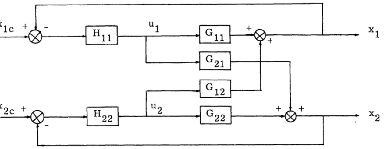
This open-loop system may be represented as shown in Fig. 2. 1.

X, 1dX2 d 1d G11] G 21d u1 _{G 11++} 1 u _ x + G(s) 1

The Open Loop Plant 2. 2

u 2 _.

2-o

The design is carried out in the frequency domain. To simplify matters for the time being, disturbance inputs are neglected. The intent

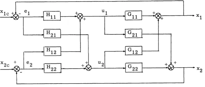
for this two-output two-control plant is to design two feedback loops as shown in Fig. 2. 2, where x- - xic _{is referred to as loop #1 and x2 ~ 2e}

as loop #2. The effect of one loop upon the other due to plant couplings is investigated in some detail, and it is decided whether this effect has bear-ing on the design of compensators H and H22'

1c + - _{H1 uG}

'_1 ₊

G21

G2

2c + H2 ₂₂ u2 _u22 , G ₂

Figure 2. 2 General Two-Loop Control System

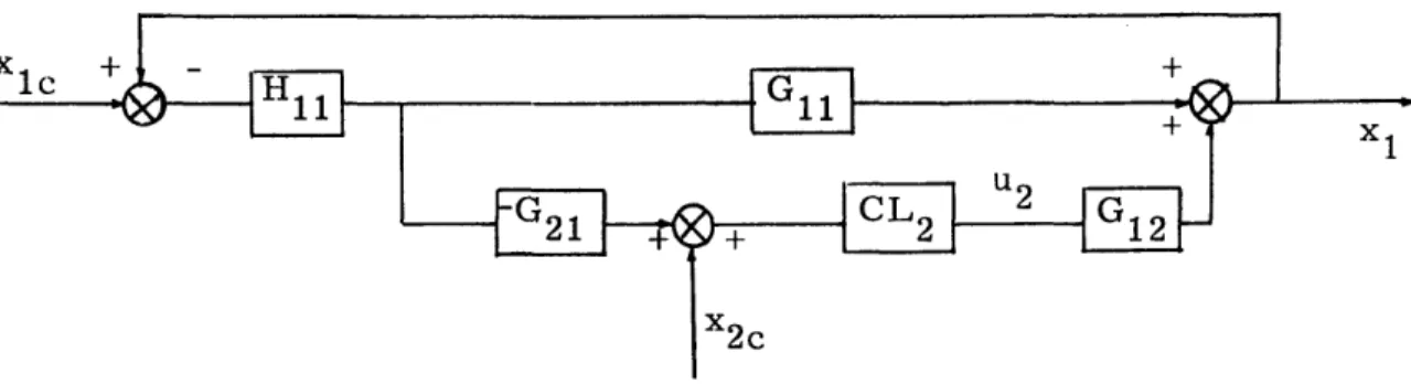
A convenient way to look separately at the coupling effects of one loop upon the other is afforded by Figs. 2. 3 and 2. 4. Fig. 2. 3 shows best the coupling effects of loop #1 on loop #2 while Fig. 2.4 shows best the effects of loop #2 on loop #1.

Figure 2. 3 Block Diagram of Loop #2 Showing Coupling from Loop #1 6

x1c +

x_2c

Figure 2. 4 Block Diagram of Loop #1 Showing Coupling from Loop #2 In Figs. 2. 3 and 2. 4,

H1 1 H2 2

CL = H and CL = 22 .

1 14H_{1 1} G_{1 2 1+H}

2 2 G2 2

The design procedure is as follows: a) Close loop #1

Design H so that the closed loop system follows the signal over a desired frequency range (generally from zero frequency up to some desired frequency), i. e., so that

1_ _{H 1 G}

T= 1 (2.4)

x1e _1+H

1 1 G1 1

over the specified frequency range. The "frequency range" referred to here is generally defined as zero frequency up to the bandwidth (WB, the half-power frequency for the closed loop) of that particular loop. The approximation that the crossover frequency (W , the frequency where the

open loop magnitude equals one) is nearly equal to the bandwidth will be used here. An additional specification for H11 is that there be adequate open loop gain margin and phase margin.

b) Analyze and design loop #2 with loop #1 closed

The closed loop transfer function for loop #2 is (see Fig. 2. 3)

2_ _{H22 (G22 - G12 L1 G21}

-(2. 5) x2c 1+H 2 2 (G2 2 - G1 2 CL G2 1)

In designing H2 2, first neglect the plant cross-coupling - the term that

represents the signal x2 passing through loop #1. The transfer function

then becomes

2 H 22 G 22 _{T (2.6)}

X2c _{1 + H}

2 2 G2 2

Design H 22' using Eq. (2. 6), to achieve the desired closed loop response for loop #2. Then, after H2 2 is designed, compare the relative sizes of

the "direct" term G22 and the coupling term -G1 2 CL 1 G2 1. Since all

transfer functions possess magnitude and phase, one must compare their vector magnitudes over the frequency range of interest. The "parameter plott" given in Appendix B is useful in this regard. An advantage to fre-quency domain design is that in doing frefre-quency, or Bode plots for the

transfer functions involved, the information regarding magnitude and phase as functions of frequency needed for the parameter plot is readily available. By using the parameter plot it can be determined whether the coupling can be neglected. If not, then it may be necessary to redesign H22 using the more complicated Eq. (2. 5).

c) Determine the effect of loop #2 on loop #1

With both loops now closed, return to loop #1 and determine the effect on x1 of the coupling caused by the closure of the second loop.

This coupling term appears in the two-closed-loop expression (from Fig 2. 4)

x1 _{H1 (G11 -G21 CL}

2 G1 2) (2. 7) 1c 2CL 1+H (G 1 - G21 CL2 G12

Analogously to b) compare, by using the parameter plot, G 1 1

and G2 1 CL 2G1 2 - the effect on loop #1 of loop #2. In many applications,

the coupling term is quite a bit smaller in vector magnitude than Gi 1, and

The notation x InCL will be used wherever there is possible ambiguity to indicate that the quantity x is being written for the system with n loops closed.

H 1 as already designed is satisfactory. However, if the coupling is large, a redesign of H1 1 using Eq. (2. 7) may have to be considered.

d) _{Determine the effects of x2c on x and x 1c on} x2

Besides coupling due to the signal of one loop passing through the other loop, there are couplings in each loop due to command inputs in the other. Of course, both these types of couplings result basically from the cross coupling plant transfer fanctions. The two closed loop "coupling" transfer functions are, again using Figs. 2. 3 and 2. 4:

x 1 _G 1 2 CL 2 (2. 8) 2c _{1 + H1 G 1 - H 1 G21CL2G12} x2 _{G 21CL 1} (2.9) X1C 1+ H _{2 2}G_{2 2} - H_{2 2}G_{1 2} CLIG _{2 1}

It will be observed throughout this paper that all transfer functions can be written in slightly different forms, each of which reveals different insights into the factors involved in the transfer functions. For instance, by simple algebra on Eq. (2. 8)

1 _{G12 L2} G x cH11G 1+GH 2c2CL 1 + G12 CL 2 2C _- H 11G211 G_{1 2} CL2 H - _{(2. 10)} H _{1 + G} H

To determine whether either of the coupling transfer functions Eqs. (2. 8) or (2. 9) is large, the form of Eq. (2. 10) is helpful. That is, if at the frequencies of interest, G - i.e., G1 2 CL2 - is much greater

than H - i.e., _L H G - H 1 1 G 2 1) - then x G12 CL 2 X2 c 1 --, which is small. H 1 "

If G << -, then - z 1. This is no surprise since G represents the

H

c plant coupling.

e) Determine the effects of disturbance inputs x ₁ and x2 on x1 and

x₂

The easiest way to obtain the transfer functions for the two-closed-loop system needed for this step in the design procedure is to use the method described in Appendix A. More will be mentioned of this method

in later chapters. Here it is sufficient to say that by this technique, the following transfer functions for disturbance inputs can be obtained:

xl d 2CL G 1d + H 22 (G2 2 G 1d -G12G21d 1 + H _{1 G 1 +} H_{2 2}G_{2 2} + H 1 1 H2 2(G 1 1 G2 2 - G1 2G2 1) Similarly, 2d 2CL x 2CL 2CL G11d _{- G} 1 2 CL ₂ G 2 1d 1 + Hi ₁ Gu 1 - H_{1 1} G1 2 CL 2G2 1 G12d _{- G} 1 2 CL 2 G 2 2d 1 + H11 _{G1 - H 1 G12 CL2 G21} G2 1d - G21 CL1G1 1 + H _{2 2}G_{2 2} - H_{2 2}G_{2 1}CLI G ₁₂ (2. 11) (2. 12) (2. 13)

loop transfer functions Eqs. (2. 11) - (2. 14) will very likely be small. But of course, if G1 1 d, G1 2 , G2 1d, and G22d are small, disturbances

will present no problem in any case. Notice that the denominators of Eqs. (2. 11) - (2. 14) (as well as the denominators of Eqs. (2. 8) and (2. 9)) will be large at low frequencies. That is, the denominators will be, at

low frequencies, approximately 1 + H 1 1 G 1 1 or 1 + H 22 G22 which, for

properly designed H_{1 1} and H_{2 2}, are large. This result contributes to making the two-closed-loop disturbance transfer functions small.

In order to get a broad view of possible types of plant dynamics and thus generate rules for making more specific predictions about couplings, the design procedure was applied to a variety of different plant dynamics. The following parameters were varied:

1. _{ratios of bandwidths of G 1 and G22} 2. _{relative magnitudes of G 1 and G22} 3. _{ratios of bandwidths of G12 and G21} 4. _{relative magnitudes of G12 and G21}

Also, it should be remembered that it is necessary to achieve small coupling only in the frequency range of interest. This range is generally from zero frequency up to the bandwidth of the loop in question. At much higher frequencies then the loop bandwidth, coupling is immaterial.

It might be of some benefit here to choose one sample case of plant dynamics - i. e., one set of parameters listed above - and apply the design procedure to it. The conclusions which will be drawn from this one qualitative case have been verified by applying the same procedure, as noted above, to many other combinations of parameters.

Consider a 2x2 plant with one high bandwidth transfer function, one low bandwidth transfer function, and two coupling transfer functions which both have moderate gain at all frequencies. Following the design procedure:

x 2G - 22 d- G 21CL1G 12 d( 2 CLG 2 (2. 14).4 2 Cd 1 + H2 2 G2 2 - H2 2 G2 1 CL1 G1 2

These transfer functions should be small in the frequency ranges of interest for a well designed system. There are several possible ways to determine whether they are large or not.

One procedure is to compare the two numerator terms in each transfer function by means of the parameter plot over the frequency range of interest (which is the frequency range of interest for the output

variable). Or, the method of Appendix A may be used to obtain the numer-ical values for the transfer functions Eqs. (2. 11) - (2. 14). This can be done fairly quickly and easily, and then frequency responses for the entire function may be done. Either way, these transfer functions do not lend themselves easily to the kind of qualitative insight as was possible in steps a) - d).

2. 3 A Summary of Qualitative Applications of the Design Procedure It would definitely be desirable if the designer, given a plant, could know whether the couplings as described previously would be large or not. This a priori information can give clues for desirable loop

clo-sure sequence.

By means of just a brief examination of the relevant transfer functions, one fortunate occurrence may be noticed. Often the plant couplings G1 2 and G2 1 appear as a product. If either one of them is

small at the right frequencies, the term containing the product will be small.

One unfortunate occurrence can also be easily recognized. It is impossible to generalize - without knowing the particular plant dynamics

-as to the size of the disturbance input transfer functions. Partially this is because each transfer function is dependent on two open loop disturbance transfer functions. One obvious conclusion is that, if the open loop

transfer functions, G 1 1 , G12 , etc. are small, then the

a) Close loop #1

Design H1 1 to be a high gain at low frequency (w <

w

H1 =K1/s.c

b) Analyze and design loop #2 with loop #1 closed

Design H2 2 to be a high gain at low frequency (w <

wc 2).

H22 K 22/s. Next, use Eq. (2. 5) to determine the effect of the coupling due to loop #1 on loop #2. _{That is, compare G2 2 and -G1 2 CL}

1 G2 1' H at low frequency (w < wc) CLH 11 L 1+H _{1 1 GH} 1 1 at high frequency (w > w c

The coupling term -G12CL1G21 is small at frequencies less than the loop #1 crossover if G 1 has large magnitude in that region. The desire here of course is that the coupling be small over the frequency range of

interest for x2, that is for W <W c . So CL should be small in this range.

This indicates that it is desirable nat c >c - that is, that the first loop have a higher bandwidth than the second. In other words, G 1 should be the high frequency transfer function of the plant, and G22 the low fre-quency transfer function. Also, it is helpful if the magnitude of the first loop (G1I) is large at low frequencies so that CL1 = /G1 1 is small.

Also, as succeeding loops are closed, the dominant factors of the denominator tend to move toward lower frequency. This, of course,

contributes to a reduction in bandwidth for each successive closure. Thus, the first loop closed should be the highest frequency loop. All of these considerations, if satisfied, will make a redesign of H2 2 unnecessary.

c) Determine the effect of loop #2 on loop #1

CL2 = H2 2 1 + H_{2 2G22} at low frequencies (w < w

)

The coupling term -G2 1 CL2 G1 2 should be smaller than G at frequencies

less than the loop #2 crossover. However, if - as was tentatively con-cluded above - Wc > , then the frequency range of interest includes higher frequencies than w c2. _{At these higher frequencies (w c<W c} CL2 ~ H22 and, since H2 2 is designed as high gain at low frequency

(W < Wc2), H2 2 may be small in this range. Also, it would be beneficial,

in order to ensure small coupling, if G22 were large at low frequency so that CL2 ~ 1/G 2 2 could be small at these frequencies. Thus, if G is large at low frequencies, then the coupling term -G2 1 CL 2 G1 2 should be

small - relative to G at least - in the frequency range of interest for x and H11 will not have to be redesigned.

d) _{Determine the effects of x2c on xI and x 1c on x}

2

From Eq. (2.8), 1 will be small if G is

x2c 1

2CL

frequencies of interest for x1(W <Wc ), assuming the sma

as discussed above.

small at

llness of CL₂ x2

From Eq. (2. 9), 2 will be small if G is small at 121

2CL

frequencies of interest for x2(w <Wc ), assuming the smallness of CL₁

The conclusions resulting from repeated applications of the design

procedure (such as the sample one just presented) for several different

combinations of plant parameters may be summarized as follows.

1.

If at least one of G12 or G

is small, or both are moderate in

magnitude, and if the "direct" transfer function G 1 is large at frequencies

of interest, then coupling can generally be neglected in the design

proce-dure. * The only notable (and symmetrical) exceptions are the following:

a)

If G21 is large and has high bandwidth, then

-

regardless of

c

b)

If G12 is large and has high bandwidth, then

-

regardless of

G

/x

c

2.

The highest frequency loop should be closed first, so that succeeding

outer loops

-

whose bandwidths are somewhat altered by inner loop

closures

-

may have as large bandwidths as possible.

3.

The "direct" transfer functions should have large magnitudes over

their respective frequency ranges of interest.

In addition, several observations can be made which would indicate

rules for a desirable loop closure sequence.

This type of conclusion is not

easy to draw and results only from insights gained from repeated

quali-tative applications of the design procedure.

1.

Since inner loops alter the dynamics of outer loops, those loops

requiring extensive compensation should be made outer loops. In this

way, the inner loops may assist in the compensation.

2.

Undesirable quantities may be suppressed by being made inner

loops. These quantities never appear outside the system

-

they are

effectively nulled by well-designed inner loops.

If any of these conditions are not met, a redesign of H

or H

may

3. The outputs of most interest - the outputs for which there will be command inputs - should appear as outer loops.

2. 4 Numerical Examples

Admittedly the application of the design procedure in the last section was a qualitative and approximate one. Here, a very simple

numerical example will be done using the design procedure. As in Section 2. 2, the plant considered has a high frequency transfer function, a low frequency transfer function, and coupling transfer functions that have moderate gain at all frequencies. Consider this plant as

G_G 1 1 G= G 21

20

The design procedure: a) Close loop #1

For H1 1 G 1 1 to have large low frequency gain, design

Hi

1

Then

T=

at low frequencies. This #1 at WB I 10 rad/sec, H _{1 1 G} 1 1 1 +H11G 100 s2+ os + 100

choice for H 1 1 also puts the bandwidth of loop

keeping this loop a high frequency loop.

b) Analyze and design loop #2 with loop #1 closed

First, neglecting coupling, design H22 so that H22G22 has a large low frequency gain. Thus

H 2 1

22

Then

T H2 2 G2 2 1

1+ H22G22 s + s +1

at low frequencies. H2 2 is designed so that WB C= 1. That is, loop

2 .2

#2 remains a low frequency loop. For this plant, an increase in the gain of H2 2 would effectively increase the bandwidth of loop #2, if desired.

Now consider the effects of loop #1 on loop #2. The coupling term is G CL G = CL = 5(s+10)

12

1 21

1

₂

_os

_{+ 100}

This coupling is fairly large at low frequency, yet H2 2 as designed for

G 22 alone is still adequate. This is evident in Figs. 2. 5a and 2. 5b which compare the frequency plots of H_{2 2} G2 2 and H2 2(G2 2 - G1 2 CL G2 1). In

these plots - and in all the frequency plots in this thesis - magnitude is plotted in decibel units (dB), where

I G(jw)IdB -

IG(jw)I

s-plane poles and zeros - contributes -180* of phase angle at dc. The coupling has the effect of reducing the crossover from C = . 80 (no coupling) to = . 50 (with coupling) and of reducing the phase

2

margin from 57* to 40*. Similarly, the bandwidth is reduced from 1. 3 to 1. 2. To reduce the coupling, it would be desirable for CL1 to be

1 -4-- -+-

r6j

log (frequency), log (w)

2. 5a Frequency Plot of H22G22

log (frequency), log (w)

Fig. 2. 5b Frequency Plot of H22(G22 - G1 2CL1 G 21

18

Lai

CL

II-smaller at low frequencies. Since CL 1 1

/G

conclusion of Section 2. 3 that G 1 1 be large at low frequencies is verified.

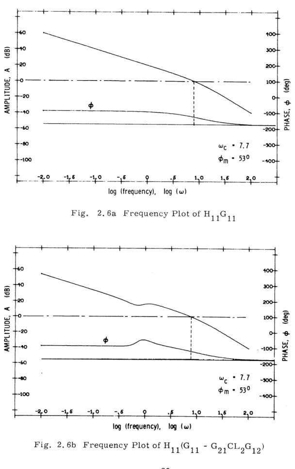
c) Determine the effect of loop #2 on loop #1 From Eq. (2. 7) the coupling term is

G2 1 CL 2G1 2 = CL 2 s2s + 1

So that

(G1 1 - G2 1 CL2 G1 2) 19s2 + 9s + 10 (2. 17) (s + 10)(s2 + s +1)

While the coupling here is fairly large, G1 1 is large enough so that there

are no difficulties. The crossover frequency and phase margin are virtually unchanged by the addition of coupling. At W = 0, G 1 1 = 2 and

the coupling term G2 1 CL2G1 2 = 1. Frequency plots comparing H11 G 1 and H1 1(G1 1 - G2 1 CL 2 G1 2) are presented in Figs. 2. 6a and 2. 6b and

indicate that the coupling is not large enough to warrant a redesign of H

1 1.

d) Determine the effects of x2c on x1 and x 1c on x2

From Eq. (2.8)

G CL s + 1

12 _{2 s2 + s + 1}

which is considerably smaller than H1 1 G1 1 at low frequencies. Thus,

the coupling effect of x2c on x1 compared to x 1c on x can be neglected

at low frequency.

From Eq. (2. 9)

G 2 1 CL 5(s + 10)

- -H-- i +___-4__ i --- i i--- -- _--

-~+io

log (frequency),

Fig. _{2. 6a Frequency Plot of H 1 G 1}

log (frequency), log (w)

Frequency Plot of H 1(G 1 - G21 CL2G12 100+ -10 L---a -20 Jc- 7. 7 <m 530 Fig. 2. 6b -300-. WO 200--1 . 1 2 0

which is considerably smaller than H2 2 G22 at low frequencies. Thus,

the coupling effect of xlc on x2 compared to x2c on x can be neglected

at low frequency.

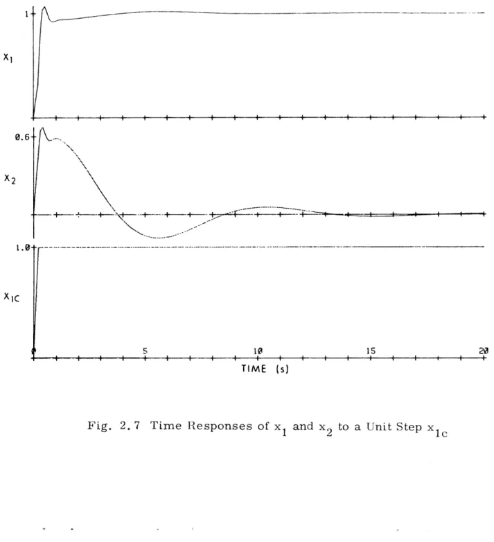
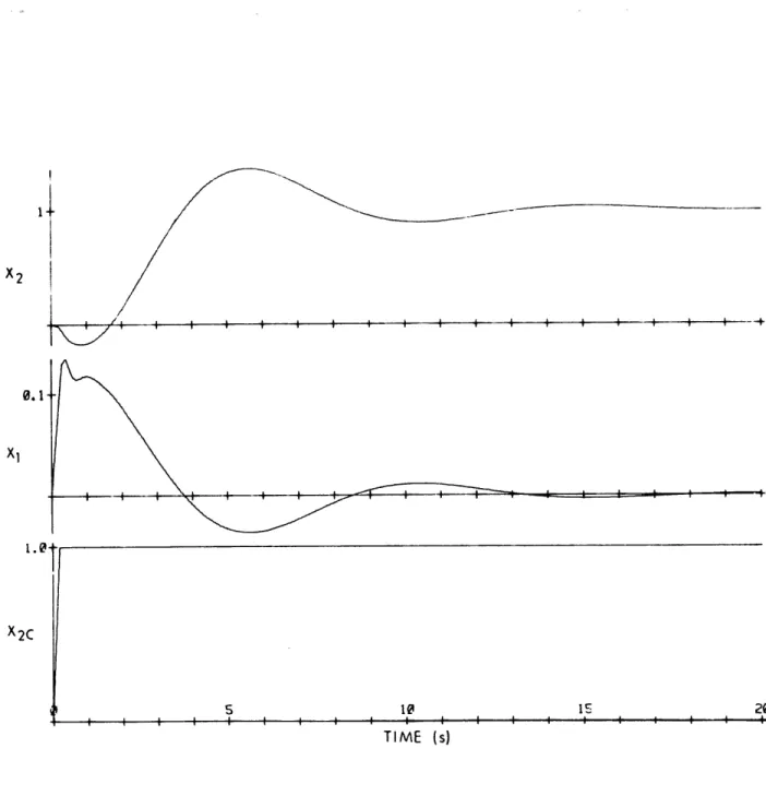
Further evidence confirming this analysis can be found in Figs. 2. 7 and 2. 8, which compare the time responses x1(t) and x2(t) due to unit step

commands x lc and x 2c* It is seen that, at steady state, the response in each loop to a command in that loop is good - i. e., the command signal is accurately reproduced. In addition, the response in each loop to a

command in the other loop is very small (zero at steady state) - indicating the small amount of coupling at low frequency.

Consider now a slightly altered plant so that G 1 1, as

has larger gain at low frequencies.

G12

G22J

The design procedure, followed in a just concluded, is recommended,

100

S+10

(2. 18)

completely parallel way to the example

a) Close loop #1 H i = 1 Then H 11 11 1, _{1 +H11G} 100 s2+ los + 100

at low frequencieswhich is exactly the same as the previous example. b) Analyze and design loop #2 with loop #1 closed

_1 H 2 2 s G=G .G 21 F--J1.

xl I I I 1 I I I I I I I i I I 0.6 X2 + - | -|-- -- + A- +-+-T I IL I - I I Xic 5 10 15 22 i 1 I I I I I I I I I I I I I I TIME (s)

Fig. 2. 7 Time Responses of x1 and x2 _{to a Unit Step x}

120

TIME (s)

Then

T - H22 G 22

2 _{1 + H22 G22}

1

s2+ s + 1

at low frequencies. The frequency plot for H2 2G2 2 is unchanged from

the first example.

The effects of loop #1 on loop #2 are the following.

G_{1 2 CL} 1G2 1 =CL -(G2 2 - G1 2 CL 1 G2 1) s + 10 s2 + 10s + 100 90 - s (s+1)(s2 4 1os + 100)

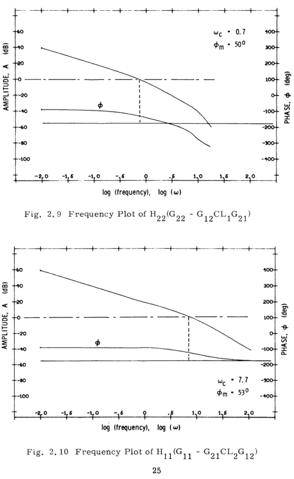
A frequency plot of H2 2(G2 2 - G1 2 CL1 G2 1) is given in Fig. 2. 9. H 22G22

is the same as in the above example, so Fig. 2. 9 may be compared with Fig. 2. 5a. This comparison indicates that the open loop transfer function for loop #2 is not significantly altered by the coupling from loop #1. The

increase in magnitude of G 1 has made the coupling term so small as to be virtually negligible, as clearly indicated in Fig. 2. 9.

c) Determine the effect of loop #2 on loop #1

G_{2 1} CL _{2 G} 1 2 = CL2 _{s ++ 1} So that (G 11 - G2 1 CL 2 G1 2) 99s2 + 89s + 90 (s + 10)(s2 + s + 1)

A frequency plot for H 1 1 (G 1 1 - G2 1 CL2 G1 2) is given in Fig. 2. 10. A

comparison of this plot and Fig. 2. 6a - which is a plot of H1 1 G 1 1 for

this example also - shows that the coupling is indeed small enough to neglect when designing H _{1 1}.

So that

(2. 19)

- -- -+-- -H---I---1---F---+-Wc * 0.7

#m

fl-4

fl-

log (frequency), log (w)

Fig. 2. 9 Frequency Plot of H 22(G22 - G 12CL G21

-60 oo--40 300--20 200- 10 0- -100-I N wm 7.1

O~m

530

log

(frequency), log

-200-

-300-

-400-Fig. 2. 10 Frequency Plot of H 1(G - G21 CL2 G12

-- 20

-60

-so

d) Determine the effects of x2c on x1 and x1C on x2

The only change from the conclusions of the above example is that CL 1 is now smaller and thus the effect of x 1c on x2 is even smaller than

previously. That is,

G CL S+ 10

21 1 _{s2 + 1os + 100}

which has a dc gain which is 1/10 of the dc gain of G2 1 CL1 in the first

example.

It should be noted that these examples are nearly "worst case" situations - the couplings are large and enter at all frequencies. The success of the design procedure for these examples is therefore quite encouraging.

CHAPTER 3

CROSSFEEDING TO ELIMINATE OR DECREASE PLANT CROSSCOUPLING

3. 1 Introduction

In certain cases of plant dynamics, as noted in Chapter 2, the coupling between loops may be significant. So that the designer may have more control over the crosscouplings than through just the design com-pensators H 1 and H2 2, crossfeeds between loops are introduced. This

is effectively compensation for the open loop coupling transfer functions G12 and G2 1. The addition of crossfeeds to the system is the major

advantage of the design procedure as presented in the remainder of this thesis. It gives the designer greater potential in eliminating unwanted couplings between loops.

In this chapter, the design procedure is expanded to include cross-feeds. Also, the factors involved in choosing effective crossfeeds

-including potentially conflicting system specifications and tradeoffs -are explored.

3. 2 First Attempt - Crossfeeding Between Error Signals

One possible means of using crossfeeds between loops to reduce plant coupling is shown in the diagram of Fig. 3. 1. Here, the error

signal of each loop is fed to the control of the other. The proposed design procedure for this system is to design the compensators H 11 and H_{2 2},

after which the crossfeeds H1 2 and H2 1 would be selected to improve

system performance and reduce coupling.

This particular scheme presents a number of obstacles and complexities which eventually result in its abandonment. First, with two-loops closed the system transfer functions are already relatively complex. It is at this point that the crossfeeds H1 2 and H2 1 are to be

122

j

Figure 3. 1 Crossfeeding from Errors to Controls in the Two-loop System

chosen. Second, the choice of the first crossfeed, whether it is H12 or H21, affects the choice of the second crossfeed. That is, the sequence of crossfeed closure is important. Furthermore, the transfer functions for the system with three loops closed are very difficult to obtain. And once determined, the transfer functions are so complex as to be not readily adaptable to the qualitative insight necessary for intelligent selection of crossfeeds.

In particular, it is found that, for three closed loops - i. e., only one crossfeed chosen - the "direct" transfer functions xi/X1c and x2 2c are in a form in which criteria for the choice of either H1 2 or H2 1 are

apparent. For example, if H12 is the first crossfeed selected, there is an obvious choice for H to improve the transfer function

-12 _{rx1c 3CL}

If this choice for H1 2 is made, however, the coupling transfer function

- _{is affected adversely.} x2c 3CL

Perhaps the degree of complexity in this scheme which makes analysis impractical for real problems can be demonstrated by an example

transfer function. One of the transfer functions for the entire system -Hi, H22, H12 and H2 1 all closed - can be written as

x 1 _ N/D X1c 4CL 1 + N/D where N/D=H G -H CLG H_{1 2} N/D = H G1 - H G12 CL2 G21+ 1 CL 2 G21 H 22 1121 H1₁₂H_{2 1} C - CL2 G1 2 + 1 H L2 G22 (3.1) H_{2 2 H11H22}

While it is apparent in Eq. (3. 1) that the first term is the "direct" term and the latter four are coupling terms, it is not obvious what the best designs for H12 and H21 are. Also, from the observation above for

the three closed-loop system, one might suspect that a good choice (in terms of Eq. (3. 1)) for H12 and H21 might cause difficulties to arise in coupling transfer functions such as - . In short, the

complex-X2c 4CL

ities - in algebra alone - inherent in this scheme for crossfeeding are sufficient to make it impractical for use in analysis and design.

3. 3 Crossfeeding Between Controls

3. 3. 1 Design Procedure for the "New Plant"

An alternate procedure to that described in the previous section is to crossfeed the control signal of each loop to the control signal of the other. Also, if the crossfeeds are chosen first, before any loops are closed, this may simplify some algebraic complexities. Ignoring for the moment disturbance inputs, this new system appears as Fig. 3. 2.

The control signal inputs to the plant are still u1 and u2'

How-ever, u₁ and u2 are now modified by the crossfeeds H12 and H21 in

the following manner:

It may be of interest to note that the H12 and H21 of the previous section are just H221 12 and H 11 H 21 respectively, here.

Two-loop System with Crossfeeds

ui = ulc + H12 u 2c

u 2 =H _{2 1u1 + u 2c}

where u lc and

equations (2. 3)

u2c are as shown in Fig. 3. 2.

may be rewritten as:

Therefore, the system

1= G 11 u1 + G12u 2 G 11 (u1e 4 H_{1 2} u₂c ) + G1 2(H2 1u1e + u2 (G 1 + H_{2 1}G_{1 2})u₁e + (G_{12 + H12 G 1)u2e} x2 = 21UI + G 22u2 = G2 1(u1e + H1 2u

)2c

Eqs. (3. 3) and (3. 4) indicate that u lc and u2c could be considered as inputs to a "new plant", which is just the original plant modified by the

crossfeeds. From these equations it is apparent that the "new plant" open loop transfer functions may be defined as:

G 1'1= G_{1 1 + H} 2 1 G1 2 G21' = G21 4 H21G22 (3. 5) G_{1 2 G1 2 + H} 1 2 G1 1 G 22'= G_{2 2 + H} 1 2 G2 1

where the control inputs to the "new plant" are u lc and u 2c. (The dis-turbance transfer function matrix Gd of course remains unchanged with crossfeeds between controls. )

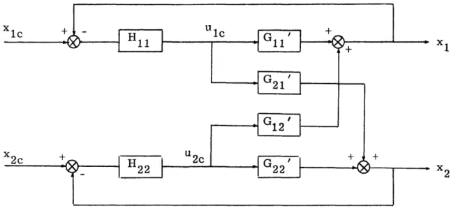
The two loop system, with crossfeeds, is now:

1c +

Figure 3. 3 Two-loop System for the "New Plant"

Before loop #1 can be closed, the designer must choose values for H12 and H2 1 which will achieve a desired degree of decoupling. Once this

is accomplished, the design procedure as outlined in Section 2. 2 is followed. The only alteration is, of course, that the new plant is used. That is, G 1 1 ,

G2 11, G1 2 ', and G2 2 ' replace Gi 1, G2 1, G1 2, and G2 2 respectively.

Also, by repeating this replacement in Figs. 2. 3 and 2. 4, those diagrams can continue to be useful in the analysis. If the crossfeeds are designed well, there is justification for expecting the design procedure for the new - and hopefully improved - plant to be very successful.

3. 3. 2 _{Choosing the Crossfeeds H}

1 2 and H2 1

Obtaining qualitative criteria for the purpose of choosing H1 2 and

H2 1 is a rather complex problem of weighing various - sometimes

con-flicting - factors. Each transfer function of the new plant is the sum of a transfer function of the original plant plus the product of a crossfeed and another original plant transfer function (see Eq. (3. 5)). The effect of the

crossfeeds on the plant in terms of frequency response is not immediately obvious. However, some conclusions about H12 and H21 can be drawn

from a knowledge of the desired amount of decoupling.

One possible choice for the designer in choosing crossfeeds is the complete elimination of any plant crosscoupling. (However impractical this may seem to be, for the purposes of this analysis one may proceed with this intent in mind. ) That is, G = G21' = 0. The crossfeeds are thus chosen so that:

G 12' G12 + HG = 0 => H 12 (3.6)

G 11

G21' G _{2 1} + H _{2 1}G _{2 2} = 0 == 21 ~ (3. 7)

G 22

This choice of crossfeeds is referred to herein as "exact decoupling". For the 2x2 case, exact decoupling completely decouples the two loops, which may then easily be designed as two separate loops.

If exact decoupling is not desired for a particular system, generally it is advantageous for the crossfeeds to at least reduce the plant cross-coupling. Thus, H12 and H21 should be designed so that G12 and G21 are altered in the direction of exact decoupling. In other words, it is desirable that G 12' < G12 and G 21' < G21 over frequencies of interest.

The crossfeeds should then be chosen so that

H 21 G22 < G21

and _{H1 2 G}

1 1 < G12

It should be remembered that the transfer functions, and in gen-eral the crossfeeds, possess both magnitude and phase. Therefore only their vector magnitudes can legitimately be compared. The parameter plot (Appendix B) is useful here. In fact, it indicates that, for instance, if the difference in phase (0 ) between G21 and H21G22 is less than 900, then G21 and H21 G22 should be of opposite sign to reduce G 21 Con-versely, if 90' < 0 < 180', then G21 and H21 G22 should have the same sign to achieve the desired reduction in coupling. These consider-ations determine the signs of H12 and H_{2 1}.

One further caution should be added here. The transfer functions and crossfeeds are generally all frequency dependent, and the design is carried out in the frequency domain. Therefore, it is necessary to satisfy the above specifications concerning vector magnitudes only over the frequency range of interest. If care is not shown in this regard it may happen that, for instance, if H21 is chosen so that G 21' < G21 at zero frequency, the magnitudes and phases ot G21' U22 and H21 change

so that G21' > G21 at higher - and still operating range - frequencies. Of course, all of the above remarks concerning G21, G 22 and H21 apply

exactly to G12, G I, and H12 _{respectively, by a symmetric change of} subscripts.

The frequency range of interest for each loop plays an important role in the choice of crossfeeds. Some of the factors summarized in Section 2. 3 help determine what the frequency range of interest is for

each loop. Low frequencies are generally of interest - the steady state response is often specified. Also, in terms of restrictions imposed on frequency ranges due to couplings:

1. If G21' is large at frequencies near the loop #2 bandwidth (WB2) then x2/ 1 0 may be significant.

2. If G 12' is large at frequencies higher than the loop #2 bandwidth (CB2), then x1/x2c may be significant.

These observations assume that, according to the conclusions of Section

2. 3, WB > WB2. Thus the relevant frequency ranges of interest (due to coupling considerations only) may be summarized as:

1. For x2, H2 1 should be chosen so that G 21' remain small

at frequencies up to the loop #2 bandwidth.

2. For x1, H1 2 should be chosen so that G1 2 ' remain small

at frequencies up to the loop #1 bandwidth.

Since G12' and G21' often appear as a product, one or the other should be small up to the highest bandwidth.

The above criteria might be simplified to state that the desire really is to make G_{1 2}' or G21' low pass in nature. That occurrence, coupled with reasonably high gains at low frequencies for G 1 ' and G22 will result in the design procedure virtually guaranteeing low frequency decoupling. Condition 2. is actually the most critical, as can be seen by considering the transfer function

x - _G

1 21CL 2 _(3.8)

x 2c 1 + H _{1 G 1 ' - H 1 G21' CL2 G12}

Since loop #2 is the lower bandwidth loop, then at higher frequencies than WB2, G2 2 ' is small. So, at these higher frequencies - which may

be less than WB1

H2

Since H22 is designed to make H 22G 22' large, H22 may very well be large at high frequency, for instance, if it supplies only phase lead. In

that case, CL 2' will pass high frequencies (i. e., frequencies above WB ' But, for the above transfer function, the frequency range of interest 2 extends beyond WB2 to WB . So unless G 12' is low pass (passing signals only up to W 2), the high frequency signal will cause the coupling Eq. (3. 8) to be very large at frequencies near the loop #1 bandwidth.

Although the crossfeeds are designed to eliminate or reduce

crosscoupling, it is apparent from Eq. (3. 5) that they also affect the direct terms G11 and G2 2. In fact, it may sometimes occur that the above

requirements on the crossfeeds conflict with some limitations on the cross-feeds derived for desirable values for G 1' and G 22'. For instance, in order for H21 G22 < G21, H21 may be of such sign and magnitude that, when H_{2 1} G_{1 2} is added to G₁i, right half s-plane zeros may appear in the resulting G 1' That is, H2 1 may be such that H21G12 > G1,

which could possibly change G 1 1 to a most undesirable G 1 1 '. The signs,

magnitudes, and phases at relevant frequencies of all terms involved must be considered in order to predict potential conflict between requirements on G 21' and G 1' _{These comments apply in a symmetric way to H}

1 2'

G12' and G22' of course.

The avoidance of right half s-plane zeros in G 'and G 22' is not their only requirement on the crossfeeds. High bandwidths and high gains are generally desirable for G1 ' and G 22' If possible, the crossfeeds should increase, or at least not decrease, both the open loop crossover frequencies and low frequency gains of G 1 and G22. High open-loop gain is especially important in view of the need to have 1 + H 1 G 1' and 1 + H2 2 G2 2' very large over low frequencies for good closed loop response.

If G 1' and G22' are large, then H11 and H2 2 will not necessarily be

This G_{1 1}' is "undesirable" because the presence of right half s-plane zeros indicate possible instability. This type of factor adds phase lag to the transfer function, thereby contributing to the possibility of reaching a phase of -180' while the magnitude is greater than one. That is, it may cause the solution of 1 + Hi G i' = 0 to be an s-plane position that has negative damping - i. e., a divergence in the time response.

designed to have excessively large magnitudes in order for 1 + H 1 G 1' and 1 + H2 2 G2 2' to be large. This desirable situation is in fact fairly

important in coupling transfer functions (see Eqs. (2. 8) and (2. 9)) where CL 1 ' and CL 2' should be small. This is of course because CL 1

/G

and CL 2' 1/G2 2' in the low frequency range.

In choosing crossfeeds, then, care should be taken not only to

ensure that the coupling transfer functions are reduced, but also to avoid

damaging and, if possible, to improve the direct transfer functions.

CHAPTER 4

DESIGN PROCEDURE FOR A GENERAL THREE-OUTPUT TWO-INPUT SYSTEM

4. 1 Introduction

In preceeding chapters, the design procedure was developed for a general two-input, two-output system. The addition of one more output variable to the system in this chapter lends, by itself, considerably more generality to the multiloop analysis. For instance, the implications of two output variables being governed by the same control are revealed. Also, the system - now 3X2 - is not amenable to matrix inversion tech-niques. Each loop closure and each possible coupling is considered sep-arately. It should be noted that the design procedure as presented assumes a knowledge of the plant.

The design procedure is presented in slightly expanded form for the three-output, two-input system. Factors involved in choosing feedbacks, evaluating couplings, and choosing crossfeeds are discussed. Conclusions are drawn from the design procedure as to exact demands to be made on

the crossfeeds.

4. 2 Deriving System Transfer Functions

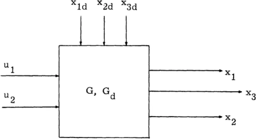
The general 3X2 plant to be considered is shown in Fig. 4. 1. For generality, it is assumed that there is a disturbance in each output

variable, i.e., that

xld

xS = ( ₂d

-2d

x3d

In order to design this system using techniques developed for the 2X2 system, it must be assumed that two of the outputs are related in some

meaningful way - by a constant factor perhaps, or by simple dynamics. It will be assumed in this chapter that x3 is closely related to x2 so that

both of them may be governed by the same control u2' 1d x2d _X3d

u 2 G, G d ' 3

x₂

Figure 4. 1 The Open Loop 3x2 Plant

For the purposes of designing feedback compensations and to keep the analysis and block diagrams relatively uncomplicated, the disturbance

inputs will, for the time being, be neglected. The effects of disturbance inputs on the system will be considered later in this section.

The system will be designed so that x1 and x2 are controlled

directly by u1 and u2' respectively, with minimum coupling. It is

assumed in doing this, as noted above, that x3 is related to x2 in such

a way that by controlling x2 with u2' x3 is also directly controlled. This

procedure allows the use of techniques developed above for the 2x2 plant. However, the presence in the system of the third output x3 implies

addi-tional considerations in the design procedure. These additional consid-erations and complexities will be examined at this point.

As developed in Chapter 3, the crossfeeds between controls u and u2 are chosen first, resulting in the new plant. Besides their affect

3 = G_{3 1} u₁ + G_{3 2 u2}

G31 (ue + H12 u2c) + G32 (u2c + H_{2 1} u1

(G3 +H 2 1 G3 2)u + (G3 2 +H 2 G3 1 )U2

Therefore, the two new plant transfer functions for x3 are

(4. 1)

G_{3 1}' G_{3 1 + H21 G32}

(4. 2) G32' _{= G32 + H12 G31}

In Fig. 4. 2 is seen the entire control system with crossfeeds chosen. There are now three loops to design.

X1c

3c

In order to proceed with the design procedure, transfer functions are needed for the complete three loop system. These transfer functions

are rather complex and the techniques used to derive them will be presented. Two methods were used to derive the transfer functions contained in this thesis. The first of these methods is basically the block diagram approach of Sections 2. 2 and 3. 3. 1. The second method (Ref. 1), referred to herein as "Multiloop Analysis" for lack of any other name, is much simpler -especially numerically - and faster and is described in detail in Appendix A. In addition, the so called "flow graph" rules could be used. However,

for this complex system this method offers no simplifications over the two previously mentioned methods.

For the first method, Fig. 4. 3 may be used. Analogous to the procedure of Sections 2. 2 and 3. 3. 1, equations for each of the output variables x, x2, and x3 can be obtained in terms of the command inputs

- x1c' x2c and x3c. It is still helpful to neglect the disturbance inputs.

Figure 4. 3 Block Diagram of 3X2 System Showing Coupling Paths

The process of using Fig. 4. 3 to obtain the overall system equations may be outlined as follows.

1= X1 G11 Gy 'ue uic +G G1'Ue4G12 u2c

x2 = G21 ule + G22 ' 2c S3 =G ₃ 1 'uIc _{+ G}

3 2' u2c

(4.3)

Then, using Fig. 4. 3,

u1e = H 1 1 x1c -H 1 1 (G 1 1' u1c + G1 2' u2e)

U2c _{CL2 x2c - CL}

2' G2 1 u 1

(4.4)

(4. 5)

It was found to be somewhat easier to continue this process considering only two loops closed, or H32 = 0. In fact, some of the two-closed-loop transfer functions generated in this way will be helpful in design. Later,

since x2c = H 32 (X3c - x3), it will be straight-forward to convert to

three-closed-loop expressions for the output variables.

Continuing by substitutina Eq. (4. 5) into Eq. (4. 4),

U1e = H 1 x1c - H_{1 1}G'1 1 u1 - H1 1 G1 2' [CL2 2c

CL

' G

'

u

l

(H