CONTROL SYSTEM DESIGN
USING H. OPTIMIZATION
by Robert Playter
B.S.A.E., Ohio State University
(1986)
SUBMITTED TO THE DEPARTMENT OF AERONAUTICS AND ASTRONAUTICS IN PARTIAL FULFILLMENT OF THE
REQUIREMENTS FOR THE DEGREE OF MASTER OF SCIENCE
at the
MASSACHUSETTS INSTITUTE OF TECHNOLOGY
June 7, 1988
( Robert Playter 1988
The author hereby grants to M.I.T. and the C.S. Draper Laboratory, Inc. per-mission to reproduce and to distribute copies of this thesis document in whole or in part. Signature of Author Certified by
K>
Cprtifpe hv Acceptedby-Department of Alronautics and/Astronautics
I / June 7, 1988
John it. Dowdle, Ph.D. Technical Staff The Charles Stark Draper Laboratory, Inc. Wallace ri. Vander Velde PrQfeslor of Aeronautics and Astronautics
Professor Harold Y. Wachman -. hairman, Departmental Graduate Committee
i SMMSASETS Immm OFTE4OLOOY SEP 07 1988 - , I A·--- -- ' I· 18 T 1 WItHRkWNr " £- we -i MA-T~~ ---JVVI Y JI
CONTROL SYSTEM DESIGN USING Hoo, OPTIMIZATION
by Robert Playter
submitted to the Department of Aeronautics and Astronautics in partial fulfillment of the requirements for the degree of Master of Science
ABSTRACT
The practical application of Ho, optimization to control system design is inves-tigated. Two solutions of the Ho, optimal control problem are presented within a general framework for control system synthesis. The synthesis approach is amenable to optimal control system design using the H2norm (LQG optimal
control) or the Ho, norm. The most recent solution to the Ho optimal control problem is significantly easier to apply than the previous solution, making the new solution a viable alternative to established multivariable control system design methodologies.
Weighting functions augmented to the open-loop system provide the nec-essary design freedom to achieve system requirements with the Ho procedure. In this thesis, system performance is achieved through singular value response shaping of the closed-loop transfer functions. Singular value inequalities are pre-sented that provide tight bounds for the response of closed-loop transfer func-tions in terms of the H,, norm and the singular value response of the weighting functions.
H, optimization is included in a control system design procedure for
large-scale interconnected systems. In a design example, the procedure is applied to an interconnected, multivariable system.
Technical Supervisor: John R. Dowdle, Ph.D.
Title: Technical Staff
The Charles Stark Draper Laboratory, Inc. Thesis Supervisor: Wallace E. Vander Velde
ACKNOWLEDGEMENT
I would like to thank the many people who have helped with the research of this thesis and, more generally, provided me with in-spiration and encouragement during my education thus far.
Dr. John Dowdle provided me with the opportunity to study at Draper Laboratory. His interest in Ho optimal control theory provided the impetus to begin my research on this topic. John's expertise, interest, and patience were invaluable to the successful completion of this project.
I thank my parents, for their ever present support, their counsel and their friendship.
I would like to thank a few special friends, and you know who you are, for providing me with the intellectual challenge and sup-port of our unique friendship. It has been, and I hope will continue to be, an inspiration to me to keep learning, and striving for the betterment of myself and those about me.
Finally, I would like to thank Eftihea. Her strength, encourage-ment and love, have been instruencourage-mental in my education in every respect.
I hereby assign my copyright of this thesis to The Charles Stark Draper Laboratory, Inc., Cambridge, Massachusetts.
Robert Playter
Permission is hereby granted by The Charles Stark Draper Lab-oratory, Inc. to the Massachusetts Institute of Technology to re-produce any or all of this thesis.
Contents
Abstract
Acknowledgement Contents
List of Figures
Notation and Abbreviations 1 Introduction 1.1 Motivation ... 1.2 Background ... 1.3 Organization ... 2 Mathematical Necessities 2.1 Function Spaces. ...
2.2 Riccati Equations and Factorizations . 3 Summary of the Solution Approach
3.1 Motivation ... 3.2 Problem Statement ... 3.3 Youla's Parametrization ... 3.4 The Generalized Distance Problem 3.5 Best Approximation ... 3.6 Summary ... 4 Problem Statement 4.1 Internal Stability ... 4.2 Youla's Parametrization ... 14
...
.16
. . . 18 ... .19...
.20
. . . 22 . ... . . . ... .224.3 Linear Fractional Transformations: Several Faces of One Problem 4.4 H, Optimization as a Generalized Distance Problem ... 4.5 Summary ... 24 25 27 28 31 34 1 2 3 3 5 5 8
5 Optimal Solutions 5.1 The H2Problem 5.2 The Ho Problem . 5.3 7--Iteration . 5.4 A Simpler Solution 5.5 Summary ...
6 Control System Design Using H-Infinity Optimization 6.1 System Definition...
6.2 Frequency Response Shaping . . 6.3 Weight Selection ...
6.4 Examples ... 7 Design Example
7.1 A Pointing and Tracking Model 7.2 Performance Bounding ...
7.2.1 Kalman Filter Bounding 7.2.2 Wiener-Hopf Bounding. 7.3 Decentralized Control Design . .
7.3.1 Stabilized Platform . . . . 7.3.2 Gimbal.
7.3.3 Fast Steering Mirror . . . 7.3.4 Performance
7.4 Ho, Design.
7.4.1 Plant Definition ... 7.4.2 Weight Selection ... 7.5 Design Examples ...
8 Conclusions and Suggestions for Further Research
35 36 37 40 44 48 49 50 52 55 56 76 77 82 82 82 84 86 86 86 91 93 93 95 98 117 . . . . . . . . . . . . . . . . . . . .
...
...
...
...
...
. . . .-...
...
...
...
...
...
...
...
...
...
...
...
...
List of Figures
3.1 Solution Methodology ... 3.2 Control System Structure ... 3.3 Standard Control Configuration ... 4.1 Standard Control Configuration ... 4.2 Modified System ...
4.3 'Subsystem of Ft(P, K)...
4.4 Modified System for Stability Analysis ...
4.5 Ft(J,Q)...
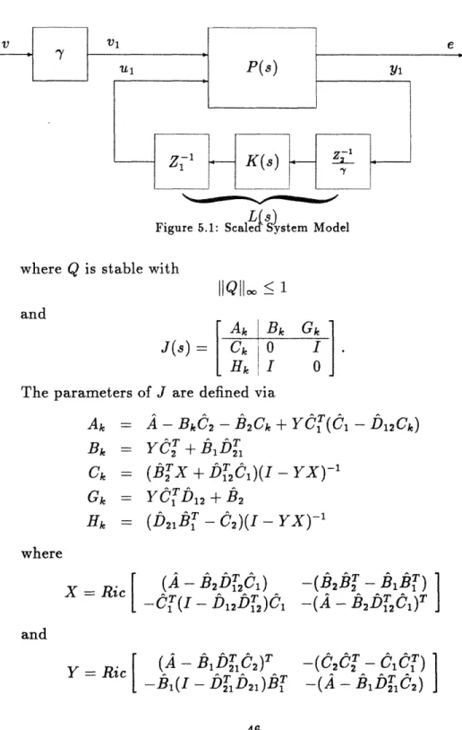
5.1 Scaled System Model ... 6.1 Control System Structure ... 6.2(a-e) Example 1 Plots . 6.3(a-e) Example 2 Plots . 6.4(a-e) Example 3 Plots . 6.5(a-e) Example 4 Plots . 6.6(a-e) Example 5 Plots .
. . . 50
...
59-61
...
62-64
...
65-67
...
68-70
...
71-73
7.1 Pointing and Tracking Model ...
7.2 Block Diagram: Pointing and Tracking Model 7.3 Loop Gains: Wiener-Hopf Controller ... 7.4 Stabilized Platform Loop ...
7.5 Stabilized Platform Loop Gain and Phase . . . 7.6 Gimbal Loop ...
7.7 Gimbal Loop Gain and Phase ... 7.8 Fast Steering Mirror Loop ...
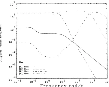
7.9 Fast Steering Mirror Loop Gain and Phase . . 7.10 Hoo Transfer Functions.
7.11 Weighted Transfer Function .. ... 7.12 Example 5-Control Loop Gains ... 7.13(a-e) Design 1 Plots ... 7.14(a-e) Design 2 Plots ...
14 16 17 24 25 26 26 29 46 77 79 85 87 88 89 90 91 92 95 96 97 99-101 102-104 . . . . . . . . . . . . . . . . . . . . . . . . . . . . . . . . . . . . . . . . . . . . . . . . . . . . . . . .
7.15(a-e) Design 3 Plots ... 106-108 7.16(a-e) Final Design Plots ... .... 111-113 7.17(a-d) H2Design Plots ... ... 115-116
NOTATION AND ABBREVIATIONS
R the real numbers C the complex numbers X complex linear space
Re(f) the real part of the complex function f Rp proper, real-rational functions
Rn xm real matrix of dimension n x m
A- 1 inverse of the matrix A
At the generalized inverse of the matrix A
A1 the orthogonal complement of the matrix A
AT transpose of the matrix A
A* Hermitian conjugate of the matrix A A > 0 the matrix A is positive definite
A O0 the matrix A is positive semi-definite Ai (A) the ith eigenvalue of the matrix A
oi(A) the ith singular value of the matrix A
a(A) the maximum singular value of the matrix A r(A) the minimum singular value of the matrix A
G'(a) := GT (-s)
the Banach space of essentially bounded matrix valued functions, F(s), with norm
IIFIIoo = e sup,, [F(jw)]
Ho: the subspace of functions F(s) in Loo which are analytic and bounded in Re a > 0
RH,o real rational functions in Ho
L2 the Hilbert space of vector valued functions with norm
IIfll2 = [o f*(jw)f(jw)dw]1 <
and inner product
< f,g >= fo f (jw)g(jw)dw
H2 the subspace of functions f(s) in L2
which are analytic and bounded in Re > 0 H,2 the orthogonal commplement of H2in L2 PH, the orthogonal projection from L2to H2
HP- the orthogonal projection from L2to H# 11112 L2 / H2 norm
IlGlloo Lo / Hoo norm
IIMII
the operator norm of MMG the multiplicative operator generated by G E Lo
MG]H2 the Laurent operator, MG, restricted to the
space of H2functions
HG the Hankel operator generated by G E Loo
Ft(P, K) the linear fractional transformation of P and K
A B ] D + C(sI - A)-'B (shorthand notation for transfer functions)
rcf right coprime factorization Icf left coprime factorization SISO single-input/single-output MIMO multiple-input/multiple-output LQG Linear Quadratic Gaussian
FDLTI finite dimensional, linear, time-invariant GDP generalized distance problem
Chapter
1
Introduction
Fundamental in the design of an optimal control system is the selection of the performance measure. This measure is generally a mathematical norm that quantifies the response of the closed-loop system. Whether or not the optimal system has desirable properties depends upon the selected norm and how pertinent it is to design goals. The H, norm is the maximum singular value over all frequency of a stable matrix transfer function. This norm provides a measure of system response that arises naturally in a broad class of input-output situations. Closed-loop systems that are Hoo optimal will thus have application to a range of important situations including the design of optimal feedback systems and ro-bustly stable systems. Another asset of Ho optimal control design is the flexibility of the framework used to define the solution ap-proach. This framework is very general and encompasses a variety of feedback problems and optimization methodologies making the approach a valuable and versatile tool. Finally, the H~ optimal control methodology offers the capability to perform explicit mul-tivariable frequency response shaping, a useful characteristic. For these reasons H,, optimal control theory is potentially an impor-tant addition to multivariable control system design methodolo-gies.
1.1 Motivation
In his seminal papers [35,36], Zames pursued the idea of H~, norm optimization of a weighted sensitivity function in order to avoid the restrictions of schemes using quadratic norms. Optimization with respect to quadratic norms, such as Wiener-Hopf and Lin-ear Quadratic Gaussian (LQG) optimal control, hinge upon the description of a particular power spectrum of the disturbance sig-nals. Performance of systems designed with this criteria tends to be sensitive to modest changes in the signal power spectrum and plant model [13,26]. The Ho norm arises when optimization over a broader class of input signals is considered, thus making
H, optimal control systems more robust to input uncertainty.
The maximum singular value has been recognized as a suffi-cient, although conservative, measure of stability in the presence of plant uncertainty [23]. The conservatism arises because of the inability to easily incorporate any known structure of the uncer-tainty. However, H, optimization, combined with the structured singular value, denoted [15], provides necessary and sufficient conditions for robust stability and performance in the presence of structured uncertainty [5]. The names i--synthesis [5] and Causal-ity Recovery Method [24] have been coined for this current topic of research.
As mentioned previously, the framework used to solve H, control problems is very flexible and can be applied to a broad class of problems. It also illustrates the inherent similarities between several different optimal control methodologies. The solution ap-proach first parametrizes all finite dimensional, linear, time invari-ant (FDLTI) compensators which stabilize a given plinvari-ant, also re-quired to have these characteristics, using Youla's parametrization. This leads to a parametrization of all stable closed-loop systems from which the optimization problem is derived. Several other op-timal control design methodologies, Weiner-Hopf or H2, which
minimizes the RMS response, and L1 [6,7] which minimizes the
maximum response, employ this general approach. The optimal solutions to H2and H, control problems are also strikingly similar.
They each require the solution of two remarkably similar Riccati equations; H2requires a single solution of two Riccati equations
while Hoo solves the Riccati equations as part of an iteration to find the optimum norm.
Finally, H,o optimization offers a capability for explicit loop shaping, and thus systematic design of closed-loop performance. Weighting functions, which act as design parameters, become, within limitations, frequency response shaping functions for selected closed-loop [25] and open-closed-loop [28] transfer functions.
1.2 Background
The H/ optimization approach to control design was introduced by Zames in [35] and developed for single-input/single-output systems by Zames and Francis in [36] where the impetus was control design in the face of disturbances and plant uncertainty. Multivariable ex-tensions of the theory have depended upon complex mathematical tools including Nevanlinna-Pick interpolation theory [9], the oper-ator theory of Sarason [29] and Adamjan, Arov, and Krein [1,2], and the geometric theory of Ball and Helton [4]. Developing a the-ory for robust stabilization with structured uncertainty has been the impetus for the Ho optimization work of Doyle and Chu who have led the practical extensions of the theory to state-space meth-ods [5,13,14,15]. These solutions are dependent upon the theory of Hankel operators and the state-space algorithms of [20]. A re-cent development by Doyle and Glover has led to a solution of the
H.o optimal control problem [16] that obviates a great deal of the
cumbersome mathematics previously necessary. It requires only the solution of two Riccati equations in an iterative procedure.
1.3 Organization
This thesis presents two solutions of the Hoo optimal control prob-lem. Application of the theory to control system design is moti-vated by a disturbance rejection problem. However, the flexibility to address different control problems is emphasized. The theory is applied to a multivariable example where solutions have been obtained using both the solution of [5] and of [16]. Design exam-ples focus on applications of the theory to shape singular value
responses of closed-loop transfer functions.
The organization of this thesis is as follows: Chapter 2 presents mathematical necessities for the solution of the Hoo optimal con-trol problem. The factorization approach of [5] is very lengthy and complex; therefore, Chapter 3 summarizes the definition of the op-timization problem and the solution approach. Chapter 4 describes the problem statement in detail. In this chapter, successive trans-formations reduce the optimization problem to a more tractable form, which is then solved in Chapter 5. A new, significantly simpler solution [16] of the H,o optimal control problem is then presented at the end of Chapter 5. Many of the complex factor-izations required for the approach of [5] are not necessary for this simpler approach, although the latter solution is presented within the same framework as the solution of [5], discussed in Chapters 3, 4 and 5. The general application of H/e optimization is discussed in Chapter 6 where the focus is on frequency response shaping of closed-loop systems. A design example for a multivariable sys-tem is included in Chapter 7, where Ho, optimization is included within a methodology for designing compensators for large-scale interconnected systems. Finally, Chapter 8 presents conclusions and suggestions for further research.
Chapter 2
Mathematical Necessities
Much of the challenge of learning H, optimization techniques is in mastering the notation and the mathematical manipulations which are used to render the problem soluble. This chapter introduces the mathematical concepts required for understanding and solv-ing the H, optimal control problem. First, the function spaces that provide the foundation of the optimization problem are de-fined. Next, matrix coprime factorizations, which are essential to this solution, are presented. Finally, solutions to Riccati equations which yield state-space formulas for the desired factorizations are discussed. The notation and properties presented in this chapter will be used throughout this thesis.2.1 Function Spaces
The H, paradigm is dependent upon the theory of Hilbert and
Banach spaces for the proof of some of its most important elements.
Two illustrations of this fact are,
* The parametrization of all stabilizing compensators for a given plant is given in terms of an unknown function Q. As long as Q is stable, i.e. belongs to to the Banach space H,, the closed-loop system is stable.
* The optimization of the H, norm of a transfer function is posed as the orthogonal projection of a function from the
Hilbert space H2to its complementary space H2L. The in-duced norm of the operator that performs this projection is the norm to be minimized.
The concepts of norm, completeness, and inner product are ad-dressed first and then used to define the desired function spaces. It is assumed that the reader is familiar with the concept of a linear space. The remainder of this section is largely taken from [18]. For a more detailed discussion of the subjects presented in this section see [11,18].
Let X denote the linear space over the complex numbers, C. A
norm on X is a function, xIIll, which maps X to the field of real
numbers, R, and has the following four properties: 1. 1111 0,
2. x11 = 0 iff x= 0,
3. Ilcxll = IclIxlJ, c E C, 4. Ixa + yll < 1l~l + IIYll.i
Completeness of a linear space is defined with the aid of a norm: a sequence {xkh} in X is said to converge to its limit, x, also in X, if
the real numbers {IIxk - x11} converge to zero as k - oo. If all the
sequences in X which tend towards convergence do so in X, then X is complete.
A Banach space is a normed linear space which is complete. There are many norms defined for a linear space populated by complex transfer function matrices. We wish to minimize the
Ho norm, (jw), the maximum over frequency of the maximum
singular value of a complex transfer function matrix. Associated with this norm are the following two Banach spaces:
Definition 2.1
Lo : The Banach space of essentially bounded (bounded
ev-erywhere ezcept possibly at a finite number of singularities) matriz valued functions, F(s), with norm
IIFIloo
= ess sup &[F(jw)].Definition 2.2
H, : The subspace of functions F(s) in L,, which are analytic and bounded in Re s > 0.
We will be working primarily with the real, rational functions in
Hoo. These matrix functions compose the subspace RH, C H,.
The definition of a Hilbert space includes the additional concept of an inner product. An inner product on the complex linear space, X, is a function denoted < , y > which maps the space X x X to the set of complex numbers C having the following properties
1. < x, x > is real and nonnegative, 2. < ,x >= Oiff =0,
3. the mapping of y to < ,y > is linear,
4. < x,y >*= < y, >,
where * denotes complex conjugate transpose.
The inner product on X may be used to define a norm,
II xI =< X,X >/2.
A Hilbert space is a normed linear space which has an inner
product and is complete.
The Hilbert spaces which we will use are now defined.
Definition 2.3
L2 : The Hilbert space of vector valued functions with norm
IIlf 112 [f, f*(jW)f (jw)dw] ' <
a)
and inner product
< f,g >=
f
f*(jw)g(jw)dw.
Definition 2.4
H2 : The subspace of functions f(s) in L2which are analytic
The H, norm is related to the H2 norm through an important and useful property. The maximum singular value is a measure of the frequency dependent gain of a transfer function matrix that is multiplied by an H2 vector. This is an induced norm of the matrix [18]. The supremum over frequency of this gain is the H, norm of the matrix. More precisely, if F E H,, then
IlFloo
= sup{llFgll2 :g E H2, 11912 < 1}.The inner product on a Hilbert space, X, also defines the con-cept of orthogonality. Two vectors x,y in X are orthogonal if < z, y > = 0. If S is a subset of X then S is the set of all vectors orthogonal to the vectors in S. If S' is closed then it is called an
orthogonal complement to S.
2.2 Riccati Equations and Factorizations
The solution of the H, optimal control problem depends heavily on transfer function matrix factorizations. The appeal of the present solution is largely due to the fact that it can be solved using state-space formulas. The relationships between solutions of Riccati equations and the desired factorizations provide this state-space capability.
The solution of certain Riccati equations are used to obtain
coprime factorizations, necessary for the parametrization of all
stabilizing compensators (Chapter 4). Special forms of coprime factorizations, inner-outer and outer-inner factorizations, are also
used to yield the generalized distance problem (Chapter 4). Finally,
spectral factorizations are necessary to solve the best approzima-tion problem (Chapter 5), the last step in the H,. optimal control
problem. The theorems of this section establish the relationships between Riccati equations and the required factorizations.
Consider the concept of coprime factorization. It is a fact [14,32] that every proper, real-rational matrix, G E Rp ( denotes the set of proper, real-rational matrices), has a right-coprime factorization
(rcj). Denote this factorization as G = NM-1. By duality a
left-coprime factorization (Icf) also exists such that G = M-lN. Definitions of right and left coprimeness follow [14,16]:
Definition 2.5 (Right Coprimeness)
Two matrices, N, M E RHo. with the same number of columns, m, are right coprime if there ezist X, Y E RHo. such that
XM + YN = Im.
(2.1)
Definition 2.6 (Left Coprimeness)
Two matrices, N, E RH,, with the same number of rows, p, are left coprime if there eist X, Y E RH.o such that
MX + NY = Ip.
(2.2)
The above definitions are equivalent to saying that the combined matrices
N
andhave a left, and respectively, a right inverse in RH.. The utility of these coprime factorizations is their capability to express every proper, real-rational matrix as a function of stable, or Hoo, factors. Equations 2.1 and 2.2 are called Bezout or Diophantine identities. The solution of certain Riccati equations will be employed to com-pute the coprime factors of Eqs. 2.1 and 2.2.
In the following, denote the transfer function matrix
G(s) = D + C(sI -A)-B
by
A B
Consider the Riccati equation
ETX + XE- XWX + Q
(2.3)
where E,W,Q E Rnn,W = WT > 0, and Q = QT with the associated Hamiltonian matrix
Denote the necessarily symmetric solution of the Riccati equation as
X =
Ric(A).-The following theorems hold [14,16].
Theorem 2.1
Let W = GGT. Then the stabilizability of (E,G) and the requirement that AH has no purely imaginary eigenvalues are both necessary and sufficient for the existence of a unique solution to Eq. 2.3 which stabilizes (E - WX).
Theorem 2.2
Let A, B, P, S, and R be matrices of compatible dimensions such that P = pT, R = RT > 0 with (A, B) stabilizable and (A, P) detectable. Then
1. The parahermitian rational matrix
(s)-[BT(_8I
- AT)-'I]
[
P
S [
(sI
-
A)-'B ]
ST
R
I
satisfies r(jw) > w. 2. For(a) E = A - BR-ST
(b) W = BR-1BT and(c) Q = P - SR
-'S
Tthere exists a unique, real, symmetric X satisfying Eq 2.3 and (E - WX) is stable.
3. There exists an M E Rp such that M- 1 E RHO and
r(s) = M*(s)RM(s).
One such M is
where F = ( + BX)
Note that 3 above provides a mechanism for performing spectral factorizations.
Next, a characterization of inner transfer functions will lead to inner-outer factorizations via the solution of a Riccati equation. Let G
[-C-
D-].
Then G is inner if G*G = I and co-inner if GG* = I. (Note that G does not need to be square.) This definition means that the singular value response of an inner or co-inner function is constant and equal to 1. An all-pass func-tion is a constant matrix times an inner (or co-inner) funcfunc-tion. If G E RX m, (p > m) is inner then G. E R(P - m) is called acomplementary inner factor if [G Gi] is square and inner. The fol-lowing result characterizes inner functions in terms of the solution of a Lyapunov equation.
Theorem 2.3 (Inner Functions)
Let G = C[
]
e Rpxm. Suppose there exists a symmetricX RnXn satisfying
1. ATX + XA + CTC = O and
2. BTX + DTC = O
Then G is inner if
3. DTD =I
The next theorem characterizes coprime factorizations with the solution of a Riccati equation.
Theorem 2.4 (Coprime Factorization)
Suppose that G =
C
- , where (A, B) is stabilizable and(A, C) is detectable. A state feedback gain, F, stabilizing
the matrix (A + BF), yields a right coprime factorization,
G = NM- 1 where
A BF BZ
[
F Z (2.4)(The notation used above means that M and N have identical
'A' and 'B' matrices but different 'C' and 'D' matrices.) A state
feedback gain, F, can be found by defining the well recognized terms of a linear quadratic regulator for Eq. 2.3:
E=A
W = BR-1B T
Q = CCT
then
F
=-R-1BTX
By duality, an output injection gain, H, which stabilizes (A+ HC), yields a left coprime factorization G = M-1N where
[ ] [A+HC H B+HD
(2.5)
[M
]
ZC Z ZD (2.5)When the requirements for an inner function are combined with a realization for coprime factorizations, a formula for an inner-outer factorization results. A function M(s) E RH, is inner-outer if M- 1 exists and is stable and proper. The next two theorems apply to stable systems. Denote by R /2 the square root matrix such that (R1/2)TR1/2 = R (or R1/2(R1/2)T = R) and let DI be any
orthogonal complement of D such that [DR- 1/2 Di] is square and
orthogonal.
Theorem 2.5 (Inner-Outer Factorization)
Assume thatG=
[
D E RHPX m (p m) is a minimalrealization of G. Then there exists a right-coprime factor-ization G = NM-', with N inner and M outer if and only
if G*G > 0 on the imaginary axis, including at infinity. A particular realization is
[
A + BF BR-1/2F
R
-1/2(2.6)
N
C + DF DR
- 1/
2R = DTD > O
F =
-R-l(BTX
+ DTC)
and
X
=
(A - BR-Ric 1 DTC) -BR-1BTCT(I -
DR-' DT)C -(A
- BR-'DTC)T
Theorem 2.6 (Complementary Inner Factor)
If p > m in Theorem 2.5, then there exists a complementary inner factor N1 such that [N N±] is square and inner. A
particular realization is
N1 =
A
+ BF
-XtCTDI
C +
DF
Di
where t denotes a generalized matrix inverse.
An outer-inner factorization is dual to the inner-outer factorization and may be determined by applying the above result to GT(s) resulting in G = /1-- 1N
Finally, an Icf with an inner denominator will be needed to perform spectral factorizations.
Theorem 2.7
There exists an Icf, G M-N, such that M is inner if and only if G has no poles on the jw axis. A particular realization is
A±HC
CH B
I D__ whereH = -YCT
andY = Ric
-A
-A
With the above theory serving as background we next turn at-tention to the Hoo optimal control problem.
Chapter 3
Summary of the Solution
Approach
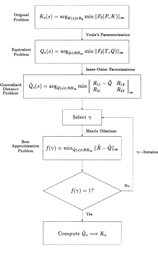
This chapter motivates the H~ optimal control problem and sum-marizes the solution. The methodology consecutively reduces the complexity of the problem until it reaches a soluble form (see Fig-ure 3.1). There are several steps in the problem reduction, and the mechanics at each step are complex. First, a general model is defined which can address a broad class of systems. The optimiza-tion problem is then stated as the minimizaoptimiza-tion of the Ho norm of a weighted closed-loop transfer function subject to closed-loop stability. The optimal compensator is denoted K,. Next, the com-pensators which stabilize the system are parametrized in terms of the stable matrix Q using the so-called Youla parametrization. This yields an equivalent but simpler representation of the closed-loop system. Employing a factorization approach, this optimiza-tion problem is transformed to a generalized distance problem. Finally, the generalized distance problem is reduced to a special form, the best approximation problem, which is solved iteratively using 7y-iteration. Once the iteration procedure has converged, the stabilizing compensator that achieves the minimum norm can
be computed. The details of these steps are found in subsequent chapters.
(Note: Most of the functions we deal with are frequency depen-dent, however the explicit dependency on s will often be suppressed for convenience).
-Iteration
Figure 3.1: Solution Methodology Origi Prob. Equiv Prob Generalized Distance Problem Appro Pr
3.1 Motivation
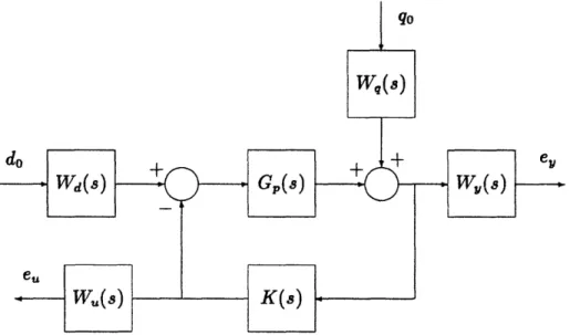
The seminal work [35,36] of Hoo optimal control addressed the min-imization of the H norm, or maximum singular value over all frequency, of a weighted sensitivity function. In Figure 3.2 this corresponds to minimizing the Hoo norm of the closed-loop trans-fer function from q to e. The equation for this is written,
e = Wy(S)S(S)Wq(S) qo
where the sensitivity transfer function is defined as
S(s) = (I + Gp(s)K(s))
-'
This problem statement allows the designer to shape the
sensitiv-Figure 3.2: Control System Structure
ity response through the choice of the weighting functions Wq and
Wy. However, it does not allow a direct method for considering
disturbance rejection or control limitations.
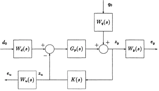
An alternative problem definition is to consider the transfer from the external signals v = [ ° ] to the weighted performance
e ]. This equation is written e,
WSWq
WuKSWq WySGpWd V. W,,KSGpWd . (3.1)Observe that with Wd and W, zero the minimization of this trans-fer function includes the original problem as a special case. A block diagram of such a system is given in Figure 3.3. This fig-ure represents the general configuration of plant and controller common to the study of Ho optimal control. All linear, lumped, time-invariant systems of interest can be expressed in this form. The plant augmented with weighting functions is denoted by P(s) and the compensator is K(s). For the systems to be considered in this thesis, the measurements, y, and the controls, u, are defined by the plant while the exogenous signal, v, consists of disturbances. The performance variable, e, defines the key variables for system optimization and evaluation.
Figure 3.3: Standard Control Configuration
In [35,36] Zames argues that minimizing the H,~ norm of the closed-loop transfer function of Figure 3.3 is preferable to mini-mizing a quadratic norm as in LQG and Wiener-Hopf optimal control. The H2 norm, a quadratic norm defined in Chapter 2, of the closed-loop system arises in two practical optimization prob-lems [5]:
1. when the input signal, v, is stochastic with a fixed power spectral density and it is desired to minimize the variance of e, and
2. when v is a fixed signal, such as the impulse response of a sta-ble transfer function, and it is desired to minimize the L2norm
of e.
These norms depend upon precise descriptions of the input signals; thus systems that are H2 optimal tend not to be robust to modest changes in the input signal.
The Hoo norm, as a measure of system response, applies to a broader class of physical circumstances, making it useful in design for performance and for robust stability. Three cases where the Hoo norm of the closed-loop system is a useful measure of optimal-ity are [5]:
1. if the input is any L2function and it is desired to minimize
the worst case L2 norm of the response, e,
2. if the input is a sinusoid and it is desired to minimize the
worst case amplitude of the response, e,
3. if robust stability is required for a nominally stable closed-loop system with plant perturbations.
In the first two cases, the set of input signals is very general and
Ho optimization minimizes the worst possible response. The last
case is important in the design of robustly stable systems.
3.2 Problem Statement
Figure 3.3 corresponds to a partitioning of the plant transfer func-tion by input and output dimensions as
P21(s ) P2()
]
(3.2)where the input-output relationships are
e(s) = P1 1(s)v(s) + P1 2(s)u(s) (3.3)
with
Pij(s) =
Di
+ C,(I - A)-'Bi.
(3.5)
The control signal is generated via feedback compensation as
u(s) = K(s)y(s).
(3.6)
The following notation will be adopted to represent the Pij in a convenient state-space format
A B1 B2
P(s)= C D .D12 (3.7) C2 D2 1 D2 2
When Eqs. 3.6 and 3.4 are used in Eq. 3.3, the closed-loop transfer function from v to e can be written as a linear fractional
transformation,
e = (P
11+ P
12K(I - P
2 2K)-P
2 1) v.
(3.8)
ore = Ft(P, K) v
The goal of the Ho optimal control problem is to design a com-pensator which minimizes the Hoo norm of this transfer function subject to internal stability of the closed-loop system:
Ko(s)
= argK(,)EnR min IFt(P, K)[oo.In what follows this optimization problem will be restated in sev-eral equivalent forms until it ultimately reaches a form that can be solved iteratively.
3.3 Youla's Parametrization
The first simplification of this problem identifies the form of the compensator to within one unknown dynamic transfer function, Q. This is the Youla parametrization of all stabilizing compensators [10,31]:
K(s) = (U + MQ)(V + NQ)
-1
(3.9)
where U, V, M, N, and Q E RH,.Youla's result states that any FDLTI compensator for an FDLTI
P(s) can be represented in the form of Eq. 3.9. The matrices
U, V, M, and N are coprime factors (Eqs. 2.1 and 2.2) of,
respec-tively, some arbitrary stabilizing compensator and the plant, P(s). Then as Q ranges over RH,, all stabilizing compensators are re-alized. (In subsequent chapters a realization of K as a function of
Q
will be found using observer and state feed-back theory. Equa-tion 3.9 can be rewritten as another linear fracEqua-tional transforma-tion which will be useful with the simple solutransforma-tion of sectransforma-tion 5.4:K = Ft(J, Q)
=
J + J
12Q(I
-
J
22Q)1J
2(3.10)
An important advantage of Youla's parametrization is that the closed-loop transfer function can be cast as a linear function of Q. When Eq. 3.9 is used in Eq. 3.8 the following linear fractional transformation results:
FI(T, Q) = Ft(P, K) = T11+ T12QT21 (3.11)
Now the objective is to find an optimal Q which minimizes the
H, norm of FI(T, Q):
Qo(s) = argQERH. min ijFt(T, Q)j,.
3.4 The Generalized Distance Problem
Further simplification of the problem utilizes the properties of
inner-outer factorizations. The Tij of Eq. 3.11 are functions of the
coprime factors U, V, M, and N. Coprime factors are not unique (see Eq. 2.4), so they can be selected such that T12 and T2l have inner-outer and outer-inner factorizations given by
T12 = N12z 12 (3.12)
and
T21 = 021N21, (3.13)
where N12 and N2l are inner and co-inner respectively and 812 and
021 are outer functions; in fact, the outer functions are constant. (Recall from Chapter 2 that an inner function is a function G(s)
such that G*G = I and an outer function is a function F(s) such that F-l(s) is stable and proper.) Additionally, the
complemen-tary inner factors NL and N can be found such that
[N12 N]
and
N21
are square and inner. The utility of these factorizations is derived from the fact that multiplication by an inner function preserves the H2and Hoo norms [14,16] and thus the norm of the closed-loop
transfer function can be rewritten as
IFt(T,Q) 11 = ]F(T, Q) [N.*
When the factorizations of T12 and T21 are applied to F(T, Q)
significant cancellations occur and the norm can be written as
IFe(T, Q)1l00 [ R11-Q R12 (3.14)
where Q is a simple function of Q. The minimization of this norm is a generalized distance problem (GDP). The name is derived from the notion of minimizing the 'distance', in an Lo, norm sense, from
R, which is an anti-stable matrix (all unstable poles), to Q which is
a stable matrix. Note that here the Lo norm is appropriate rather than the Hoo norm because the matrix is no longer stable. For the case in which R is a real-rational matrix an optimum solution is known to exist [14,16]. However, the proof of existence does
not yield computable formulas. Thus the final step in solving the problem is to reduce the generalized distance problem to a best (or
Hankel) approximation problem.
3.5 Best Approximation
The generalized distance problem is reduced to solving a series of best approximation problems [1,2,20,29] using matrix dilation
theory in a process called --iteration. The optimization problem is written as
min R1 1-Q R1 2
1
~(o)¢/RHo R21 R22 ]|'
The iterative procedure is initialized by using an estimate of the optimal norm, 7. Then applying the properties of matrix dilation [8,14] to Eq. 3.15 the following 'one-block' problem results:
f(y) min IR - 0lloo (3.16)
0(a)ERH0 0
where R is a function of the Rij in Eq. 3.15 and -y. The initializing y is less than yo if and only if f(y) < 1. If y is selected to be exactly equal to the optimum norm then the one-block problem will yield f(7y) = 1. Thus yo can be found from the zero crossing of the function f ()- 1. is updated, using bisection for example, according to the value of f ().
Equation 3.16 is called a 'best approximation' problem because we are approximating an antistable matrix, R, by a stable matrix, Q, while minimizing the L, norm of the difference. Clearly this is a special 'one block' case of the generalized distance problem. The approximation is equivalent to a projection using the Hankel
operator. Therefore, f(y) is equal to the Hankel norm of R. Once
the optimum cost is known, a Q, which achieves the L norm, can be determined using state-space methods [20]. Then Q,, Qo and
Ko are computed by inverting the necessary transformations. The
resulting frequency response of FI(P, K) has constant maximum singular value response equal to 7y.
3.6
Summary
This chapter has described the solution to the H, optimal control problem at a very high level as the minimization of the H, norm of FI(P,K)over all stabilizing compensators in Rp. The Youla parametrization, the generalized distance problem, 7--iteration,
and best approximation problems were presented as key steps to-ward obtaining an Ho optimal compensator. In the chapters which
follow, details of the computational procedures required in carrying out these steps are presented.
Chapter 4
Problem Statement
This chapter contains the detailed statement of the H~, optimal control problem. Requirements for internal stability and 'optimal' performance are set forth. The optimization problem itself can be represented in several distinct forms; equivalent representations will be employed which sequentially reduce the complexity of the problem until a soluble form is reached. The major results of this chapter are quickly previewed.
The configuration of plant and compensator that will be used is shown again in Figure 4.1. The goal of H~ optimization is to find
Figure 4.1: Standard Control Configuration
the closed-loop transfer function, Ft(P, K). Youla's parametriza-tion yields a linear fracparametriza-tional transformaparametriza-tion, FI(J, Q), for all lin-ear, time invariant, finite dimensional compensators which stabi-lize the given system. Then a linear fractional transformation for the closed-loop transfer function that is linear in Q, FI(T, Q), is derived. Special forms of coprime factorizations, namely inner-outer and inner-outer-inner factorizations, then allow the optimization problem to be cast as a generalized distance problem. State-space formulas for the required steps are provided.
4.1 Internal Stability
To aid in the definition of internal stability, introduce two fictitious signals wl and w2as in Figure 4.2. To insure that the transfer
func-Figure 4.2: Modified System
tion from v, wl, and w2to u exists and is proper, (I-P 22(oo)K(oo))
must be invertible [5,14]. This condition for well posedness is as-sumed in the remainder of this thesis. If the transfer functions from wl, w2, and v to e, u and y are stable then the system is
considered internally stable. Alternatively, let v be set to zero in Figure 4.1. The system is considered internally stable if the state vectors of P(s) and K(s) tend to zero from every initial condition. (This is the usual definition of asymptotic stability.)
It is a fact [5,14] that the system of Figure 4.1 is internally stable if and only if the system of Figure 4.3 is internally stable. This becomes intuitive when v is set to zero as previously described;
in this case the only feedback loop involves P22 and K. In the
following, the system of Figure 4.3 will be used to characterize closed-loop stability for the entire system.
Figure 4.3: Subsystem of Ft(P, K)
Consider the system of Figure 4.4. The input-output relation-ships for this system are given by
[
-P22 I
[:e2
=
[:
(4.1) This system is internally stable if and only if the following transfer function matrix is stable:
I
-K
1_
I + K(I
-
P22K)-1P22
K(I
-P
22K)-1
-P
2 2=
(I - P
22K)-P
2(I -
P
22K)-1
(4.2) Therefore, the closed-loop system of Figure 4.1 is internally stable if and only if the matrix of Eq. 4.2 is an element of RH. Youla's parametrization provides an equation for the compensator that insures that this requirement is satisfied.
4.2 Youla's Parametrization
Youla's parametrization is presented here in a general form; it re-quires knowledge of the plant and some arbitrary stabilizing com-pensator. The result is an equation, with one free transfer ma-trix, Q RH,, that defines all compensators which stabilize the
closed-loop system. In the next section a particular form of Youla's parametrization is defined using gains derived from observer and state feedback theory.
Recall from Chapter 2 that every proper, real-rational matrix has a right and left coprime factorization [14]. Begin with right and left coprime factorizations of P22 and Ka, some stabilizing
compensator:
P22
= NM
-1= -1 N
(4.3)
Ka
= UV-1 =
fV-1U(4.4)
Substituting these expressions into the left hand side of Eq. 4.2 results in
o
]
-
=
]
-0
(4.5) For the system of Figure 4.1 to be internally stable, both of the block matrices on the right hand side of Eq. 4.5 must be in RH,. The right-most matrix of Eq. 4.5 is clearly stable by virtue of the fact that coprime factors are stable.
When the factorizations of Eq. 4.3 and 4.4 simultaneously sat-isfy Bezout identities (Eqs. 2.1 and 2.2) the following equation, often called the double bezout identity, holds:
[U
M
N
V
f
[
I
]
(4.6)
or
V
-t
e = N V
From this expression it can be immediately deduced that the in-verted matrix on the right hand side of Eq. 4.5 is stable by the inverse defined in Eq. 4.6, again because the coprime factors are
stable. Therefore, any Ka and P22 combination whose coprime
factorizations satisfy Eq. 4.6 yield an internally stable system. If instead of using the coprime factorizations of Eq. 4.4, we use
Uo=-U+MQ
V =V+NQ
UO= U+QM
VzV + N
then the double bezout identity of Equation 4.6 is still satisfied for any Q C RH,,. By using the above characterization of the coprime factors of K, the parametrization of all stabilizing compensators is given by the following right and left coprime factorizations
K = (U + MQ)(V + NQ)
-1 = (X/ + QN)-(U + QMT) (4.7)
which is the desired result.
4.3 Linear Fractional Transformations: Several
Faces of One Problem
The previous section utilized coprime factorizations to show that all stabilizing compensators can be parametrized by one simple formula, Eq. 4.7. This section uses that form to show that the compensator and the closed-loop transfer function can both be rep-resented by linear fractional transformations. Realizations of these equations will be given using the state-space formulas of Chapter 2.
Recall that the closed-loop transfer function is given by the linear fractional transformation,
Ft(P, K)
= P11+ P12K(I
-P
2 2K)-P
2,
1.
(4.8) Youla's parametrization led to an expression for all stabilizing com-pensators, which is itself a linear fractional transformation. It can be shown [14] that Eq. 4.7 can be written asor
K = FI(J, Q) = J11 + J12Q(I -
J
22Q)-J 21 (4.9) whereJ = UV-
(4.10)-V"'N
The linear fractional transformation for the compensator is repre-sented pictorially in Figure 4.5. A stabilizing compensator may be
Figure 4.5: Ft(J, Q) found by computing the coprime
the realization of P22,
factors of Eq. 4.10. Begin with
P =
A
22P22=[C2 D22
A stabilizing state feedback gain, F, and output injection gain, H, yield right and left coprime factorizations via Eqs. 2.4 and 2.5:
P
22= NM-
1=
M-1N
+]
[
A + B
2F
B2 C2 + D22F D22 A + HC2 C2IH
I
B2+ HD22 (4.11) (4.12) D2 2 piB V-]The factors of Eq. 4.10 are derived from the model based com-pensator associated with F and H, which is realized by the state equations
= A +
B
2u + H(C
2+
D
22u
-y)
u = F.
This compensator has the state-space representation
K.
A + B2F+HC2
+
HD22F -H
F
0]
To identify an rcf and an Icf for this compensator define
A
= A+B
2F+HC2 + HD
22F
b = -H
C = F
1D = 0 tF = C2 + D22Ft = -(B
2+
HD
22)
Then, using Eqs. 2.4 and 2.5, the coprime factorizations of the model based compensator are identified in terms of the state-space parameters of P2 2:
A±B
2F -H
C2 + D22F I (4.13)
F 0
[V ~] = [ A +
HC2-(B
2+ HD
2) -H
(4.14)
With these factorizations available, a realization of J, and thus of all stabilizing compensators, is immediate. When Eqs. 4.11, 4.13, and 4.14 are applied to Eq. 4.10, the following representation of J results:
A
+
B
2F + HC
2+ HD
22F -H B2 + HD
22J=
F
0
I
We can go one step further with the approach of linear frac-tional transformations. Using Eqs. 4.3, 4.6 and 4.7, the following expression for the closed-loop transfer is obtained:
FI(P, K) = (P
11+ P
12UIUMP
2 1) + (P
12M)Q(MP
21).
This is itself a linear fractional transformation. The importance of this particularly simple form for the closed-loop transfer function is that it is linear in Q:
F
t(P, K) = FL(T,
Q) = T
1+ T
12QT
2 1 whereT=[P1
+ P
12UMP
21P
12M
MP21 °
Realizations of the Tij can be found from the realizations of the Pj and the coprime factors of P22 and K0
[5].
After muchsimplification, the Tij can be represented as
A + B
2F
-HC
2-HD21
Tn =
0
A + HC
2B + HD21
(4.15)
C1 + D12F C1 Dll T12 = C A[ z D+ 2 12F (4.16) and A + HC2 B1 +HD2 1 T21= [ C 2 D2 1 (4.17)4.4 Ho Optimization as a Generalized Distance
Problem
In the previous section a particular realization of Youla's parame-trization of all stabilizing compensators was used to derive state-space formulas for all stabilizing compensators, F(J, Q), and all stable closed-loop systems, Ft(T,Q). A state feedback gain, F, and an output injection gain, H, for the subsystem P22 were used
on the derivation of F and H yield forms for T12 and T21 of Ft(T, Q) that are particularly useful. These are an inner-outer
fac-torization of T12 and an outer-inner factorization of T21. They allow
the optimization of the transfer function, FI(T, Q), to be stated in terms of a generalized distance problem.
The inner-outer factorization of T12 is given by T12 = N12Z17
-The complementary inner function, N±, is also found such that
T12 = [N1 2 N]
[
]
where
[N12N]
is square and inner. The outer function Z1 is a constant matrix.
Similarly, the outer-inner factorization of T21 and the complemen-tary inner function, N1 are found such that
1 = [Z1 0o]
[21
whereiN21
is square and inner and Z2 is a constant. The utility of these
fac-torizations lies in the fact that multiplication by an inner function is norm preserving [14,16]. Thus
F(T,Q)11.
=[
12
FI(T, Q) [2
1N]
Using the inner-outer and outer-inner factorizations of the Tij the argument simplifies to the form of the generalized distance problem,
IIFt(T, Q)l = R11 -Q R122 I (4.18)
where
R1 = N;2T11N2 (4.19)
R2 = N;T 11N*1 (4.21)
R22 = NjT
11Ni
(4.22)
and
Q
= -ZlQZ_ -. (4.23) The convenience of the constant outer functions is apparent when Q needs to be computed from a realization of Q. For the case of constant outer functions, the required inversions are very simple. State-space realizations of the required factorizations result from Theorems 2.5 and 2.6.If T12 is an n x r matrix and n > r then the complementary
inner factor, NL, may also be found. Applying Theorems 2.5 and 2.6 gives the following form for an inner-outer factorization of T12
with complementary inner factor:
Tl2 = [N12 N]
[
(4.24) Z1 = (DTD- 12) 1/2 (4.25)[N
12N]
[
A+B
2F
B
2Z
1 XC (4.26) withD±DT = I - D
12ZlZ[
D2
(4.27)
F is given byF = -Z
1Z[ (BX + DT2C)
(4.28)
andX
=Ric [ A-
B2Z1 ZTDTC -B2Z 1ZTBT-CTDIDTC
1-(A - B
2Z
1ZTDC
1)
T (4.29) Note that D12 must be full rank so that Zl is non-singular.Duality principles may be applied to obtain the outer-inner fac-torization of T21 E RXm, p < m. If p < m the complementary
inner factor, N1 can also be found:
Z2 = (D21D21 A+HC 2 B1 Z2C2
-DLBTYt
bTb =
I
- DZT:Z
2D2 1 -H is given byH
= -(YC
2+ B,
1D:)Z
212~luZ
2 and - B1DTZT Z2C2)T -B 1DTDB BT -C2Z2 Z2C2-(A - BDTZTZ2C)
'
(4.35) Similarly, D21 must be full rank so that Z2 is non-singular.4.5 Summary
Using the results of this chapter, all FDLTI stabilizing compen-sators are parametrized by a linear fractional transformation. In addition, the closed-loop transfer function is parametrized by a sin-gle linear fractional transformation that is linear in Q. This latter expression allows the optimization problem to be cast into a gener-alized distance problem. State-space formulas for the computation of all necessary transformations have been provided.
The solution of the generalized distance problem is the subject of the next chapter.
N 2 1i L N with + HD2 1 Z2D21
Dl
(4.31)I
(4.32) (4.33)Y= Ric (A
(4.34)Chapter 5
Optimal Solutions
Youla's parametrization and the factorization approach of Chap-ter 4 have allowed the optimization problem to be cast as a gen-eralized distance problem. This chapter is devoted to the solution of this problem.
All the transformations of the problem to this point are actu-ally independent of whether the H2 norm or the Ho, norm is cho-sen as the measure of optimality for the GDP since both norms are invariant to transformations by inner functions. Therefore, the framework of this procedure can be used to solve either
optimiza-tion problem. Considering this generalizaoptimiza-tion, the GDP is stated as the minimization of
1FI(T, Q)11a - R 1 1- R12
R
21R22(5.1)
where a equal to 2 or oo refers to the H2 or Ho, optimization prob-lem. The H2 optimization problem is equivalent to solving a Linear Quadratic Gaussian (LQG) problem with, potentially, frequency dependent weighting functions [3,21]. Its solution is particularly simple at this point and is equivalent to solving a projection prob-lem. There is also an indication that this form of the H2 solution may obviate difficulties associated with the LQG/LTR (Linear Quadratic Gaussian with Loop Transfer Recovery) method, such as requiring infinite gains to adequately recover the target loop [30]. The Ho, solution being addressed here is more complex and involves the solution of a related best approximation problem.
In this chapter, the existence of a solution to the GDP will be discussed briefly. An abstract operator point of view is employed which utilizes the 'geometry' of the problem. This operator per-spective leads to a solution for a very special case of GDP, the 'one-block' problem. More general cases, two and four-block prob-lems, that result from Hoo optimization must be solved by itera-tively reducing the problem to a one-block problem in a process called 7--iteration.
This chapter concludes with a brief presentation of the latest solution to the H, optimization problem [16], which drastically simplifies the solution procedure. This is the solution that was most easily applied to the design example of this thesis (see Chap-ters 6 and 7).
5.1 The
H
2Problem
In order to demonstrate the utility of the generalized distance prob-lem formulation, we first consider the H2problem. The H2 norm
of the closed-loop system may be represented by
IIF(T, Q)12 = R -Q
-
R12R2 1 R2 2 2
The optimization of JIFt(T, Q)112 is particularly simple because
R1 1-Q R12 2 =-IR 11 2-QI+ R21 R22
R2 2 2 2
and the optimal Q is merely the stable part of R11 [16]. Since R11
is completely unstable Qo is equal to the constant part of R11:
Qo = Z1D12D1 1D2 1Z2.
The optimal Q is found by inverting the transformation of Eq. 4.23, which results in
Qo =
-D12DljD21-The optimal H2 compensator can now be found by employing the realization of F( J, Q) .
5.2 The Hoo Problem
We now consider utilizing the generalized distance problem formu-lation to solve the Hoo optimal control problem. Recall that the problem in its present form was obtained by factoring the linear fractional transformation,
F(T,
Q)
=T
11+
T 2QT21.A sufficient condition for the existence of an optimal solution is given below [17].
Theorem 5.1
The optimal Ho norm of FI(T, Q)is achieved if the matrices T12 and T21 are full rank for all frequencies.
(These conditions usually hold for well-defined problems.)
The optimization problem calls for minimizing the 'distance', in an Loo norm sense, from a stable matrix Q E Ho to the antistable matrix R E Lo,. (Note that the L,o norm is required because R is unstable.) Let us examine the simplest case first.
If T12 and T21 are both square and full rank, then so are their
inner factors, N12 and N21, which implies the complementary inner
functions Nl and Nj do not exist. In this case R11 is the only
non-zero element of R (see Eqs. 4.19-4.22). The Hoo optimization problem in this case is equivalent to the one-block problem given by
IIF(P,K)IIo = IIR1- Qll (5.2)
and a Qo that achieves the optimum is sought. This is the so-called best appoximation problem, and its solution is central to the solution of the general case. Therefore, we examine it in some
detail starting with the operator theoretic perspective.
H2is a closed subspace of L2; let Hjldenote its orthogonal
com-plement. The multiplicative operator associated with a matrix R1 E Lx is referred to as the Laurent operator and, when
operat-ing on a function f E L2, is denoted by MR,: