Cost Estimation of Functional and Physical Changes
Made to Complex Systems
by
Peter Nicholas Jeziorek
B.S. Mechanical Engineering
University of California, Los Angeles, 2003
SUBMITTED TO THE DEPARTMENT OF MECHANICAL ENGINEERING IN
PARTIAL FULFILLMENT OF THE REQUIREMENTS FOR THE DEGREE OF
MASTER OF SCIENCE IN MECHANICAL ENGINEERING
AT THE
MASSACHUSETTS INSTITUTE OF TECHNOLOGY
FEBRUARY 2005
C 2004 Massachusetts Institute of Technology. All rights reserved.
Signature of Author:
~~rtme~At of Mechanical Engineering
January 14, 2005
Certified by:
V 1
9
Ralph E & Eloise F Croyrofessor
Nam P. Suh
of Mechanical Engineering
Thesis Supervisor
Accepted by:
MWASSACHUSETT INSTrTUT
OF TECHNOLOGYMAY
5 2005
LIBRARIES
Lallit Anand
Professor of Mechanical Engineering
Chairman, Committee for Graduate Students
Cost Estimation of Functional and Physical Changes
Made to Complex Systems
by
Peter Nicholas Jeziorek
Submitted to the Department of Mechanical Engineering On January 14, 2005 in Partial Fulfillment of the Requirements for the Degree of Master of Science in
Mechanical Engineering
Abstract
Current cost estimation practices rely on statistically relating physical parameters of a system to historical cost data. Unfortunately, this method is unable to effectively communicate the increasing complexity of system design to cost data. Additionally, current cost estimation techniques have had a historical inability to produce credible and explainable results. It is often considered to be a "black art" with the recurring question: "Where did that number come from?" This thesis systematically links design and cost information together, and demonstrates the utility of that link by estimating the impact of functional and physical design changes on the life-cycle cost and determining key cost drivers. The ability to quickly estimate the cost impact of design changes is important for decision makers and serves as a medium of communication between customers and developers.
Credible estimation is gained by intimately linking the axiomatic design framework to the already existing costing unit (or component) domain and providing design traceability.
Development cost is predicted by determining the functional requirements (FRs) affected by a change in customer needs or constraints, then by determining the propagation of that change from FRs to design parameters (DPs) to costing units. The list of affected components and the magnitude of the impact on each component is found and then used to determine through a parallel iteration process model how much development labor will be necessary to implement those changes. The labor is directly related to development costs.
A formal method to designing operations using axiomatic design is presented in this thesis. Operations exist due to the time-variant combinatorial complexity of FRs. Operations implement reinitialization procedures in order to maximize the probability of success of FRs. This provides the way that axiomatic design can derive operations and the related cost parameters. This information could then be plugged into the cost impact model of a design change to determine the list of affected operations. A new method of estimating the change in cost parameters due to a design change will be the focus of future research.
Two main forms of key cost drivers are identified: the most expensive FRs and design iteration. A method of mapping estimates from the costing unit domain to the FR-DP map is suggested in order to cost out FRs. Design iteration as a key cost driver can be seen from two points of view. Axiomatic design identifies small design ranges, coupling and imaginary complexity as contributors tocoesfisign structvre matrices identify the most iterative set of tasks in the development process and offer procedures to reduce or speed up the iteration.
Thesis Supervisor: Nam P. Suh
Acknowledgements
The day I came in to interview for this project, I had absolutely no knowledge of axiomatic design whatsoever. Now after almost nine months, I am able to tackle such difficult design problems such as robustness and complexity. I would not have been able to grow as fast as
I had without the help of Professor Nam P. Suh and Taesik Lee.
I'd like to thank Professor Suh for overseeing this project. He has always been a strong
supporter of the project, and stood by the cost estimation method that I developed along with Taesik. His style of management has helped me to become an independent thinker and researcher.
I am not just regurgitating the ideas of others, but creating new ones. With just one short line
from Professor Suh like "Why don't you think about this a little more" or "That's it, huh?" I will add another ten pages to my thesis!
I'd like to thank Taesik Lee for all the discussions we've had concerning axiomatic
design and even various matters of life. Often I wouldn't even know what I was trying to say until
I tried conveying it to Taesik. He would sit there silent for five minutes and then give some very
powerful insight. Without Taesik, this project would have gone nowhere fast. Instead, we hit the ground running and though we slowed down midway, we will be ready to pick up the pace once again to finish the race in first place.
I'd like to thank Lockheed Martin for their support on this project: Robert Ford, Ray
Damaso, Chip Woods, Rich Freeman, and Gregory Kerhl. Constant dialogue between MIT and Lockheed has pushed this project forward, making it a very practical and cutting-edge cost estimation tool. I'd like to especially thank Chip Woods for all his correspondence and feedback.
I'd like to thank all the people at Axiomatic Design Solutions Inc. (ADSI): Matt Pallaver,
Christian Arangio, and Sung Hee Do. I appreciate all the discussions and the endless number of questions that you guys have.
Thank you Steven D. Eppinger for the presentation you made at ADSI and the discussion that we had thereafter. Your insight and work have been indispensable.
I'd finally like to thank all my lab mates Hrishikesh Deo, Beto Peliks, and AJ Schrauth,
for their constant cheer and rowdiness brought to the environment. Without them I would have been done several months ago, but it wouldn't have been half as fun. Thanks Hrishikesh for all your in-depth discussion about Axiomatic Design and Mechanical Engineering. I can always
count on you to know what I'm talking about within a few minutes and have good feedback. Thank you mom and dad. Thank you for your overwhelming support in whatever I do. I respect and love both of you. You are both champion parents and are capable of parenting even the most challenging sons: Alek and I!
Finally I'd like to thank Victoria Tai for all her love and support. She is main the reason I am here at MIT today, and is the reason I am continuing on for a Ph.D. Vicky instantly realized my potential, when I could not. She is an inspiration and an amazing person to spend all my time with. Thank you, Vicky!
I've learned so much, even about the process of learning itself. Learning floats vague ideas somewhere in the depths of your mind. Writing down the idea makes you realize all the problems. You address those problems with countless scribbles and thrown away scraps of paper. Finally, you present the finalized, internalized idea a hundred times. I hope to never stop learning.
Table of Contents
A BSTRACT ... 2
ACK NO W LEDG EM ENTS... 3
TA BLE O F CO N TEN TS ... 4
CH APTER 1 ... 6
IN TRO DUCTION ... 6
THE N EED FOR COST ESTIMATION ... 6
THE CURRENT STATE OF COST ESTIMATION ... 7
THESIS OBJECTIVE ... 8
COST BACKGROUND AND TERMINOLOGY ... 8
1. D evelopm ent ... 9
2. Production ... 9
3. Operation ... 9
SUMMARY ... 10
CH APTER 2 ... 12
ENHANCING THE CREDIBILITY OF COST ESTIMATION WITH AXIOMATIC DESIGN...12
AN INTRODUCTION TO AXIOMATIC DESIGN ... 12
CONNECTING DESIGN AND COST INFORMATION ... 15
TRACEABILITY ... 15
SUMMARY ... 17
CH APTER 3 ... 19
QUICKLY ESTIMATING THE COST IMPACT OF A DESIGN CHANGE TO DEVELOPMENT ... 19
IDENTIFY THE COMPONENTS AFFECTED BY A FUNCTIONAL CHANGE... 19
DETERMINE THE DEVELOPMENT LABOR COST ... 25
ESTIMATE THE COST IMPACT OF A DESIGN CHANGE ... 29
SUMMARY ... 33
CH A PTER 4 ... 35
O PERA TIO NS CO ST ... 35
AN INTRODUCTION TO COMPLEXITY ... 35
AXIOMATIC DESIGN OF OPERATIONS ... 38
COST OF OPERATION ... 39
SUMMARY ... 43
CH APTER 5 ... 44
K EY CO ST DRIV ERS ... 44
THE COST OF FUNCTIONAL REQUIREMENTS ... 44
DESIGN ITERATION ... 45
Axiomatic D esign -D iscussion on D esign Iteration ... 45
D esign Structure M atrices -D iscussion on D esign Iteration ... 49
SUMMARY ... 50
CH APTER 6 ... 52
SUGGESTIONS FOR FUTURE RESEARCH ... 53 G LO SSA RY O F TER M S ... 55 A PPEN D IX - M A TLA B C O D E ... 56 MAINSCRIPTA ... 56 CREATEPOSSIBLEM ATRICESM ... 58 DETERMINESEQUENCESM ... 60
EXPECTEDN UMBERO FITERATIONS.M ... 61
Chapter 1
Introduction
One of the largest difficulties in developing complex systems is managing and estimating the cost. Life-cycle cost is a measure of the total cost of a system in each phase of its existence: development, production and operation. By knowing the life-cycle cost of a product one can make a decision on whether to proceed with the development of the system or not. This
knowledge of the life-cycle cost is invaluable, and can determine the future success or failure of a system. The following examples illustrate the current need for accurate life-cycle cost estimates in complex systems.
The Need for Cost Estimation
In early 1969, Ingalls Shipbuilding Company, by far the largest shipyard in the world, received a contract from the United States Navy to build nine amphibious assault ships (LHAs) for a firm fixed price. The LHA is 20 stories high and the length of three football fields and is capable of deploying 2000 fully-equipped Marines and 200 combat vehicles via landing craft and
30 large helicopters. By the Navy's standards, the LHA was "the largest, fastest and most
versatile vessel in the history of American amphibious warfare." In the mid 1970s, Ingalls received another contract from the Navy to produce 30 DD963 Spruance-class destroyers. Ingalls more than doubled its workforce to take on both programs. At the onset of each project, the Navy had only given Ingalls performance specifications of each ship. As a result, at each phase of Ingalls' development process, the Navy interfered by suggesting hundreds of design changes that caused an increase in the amount of work needed to be accomplished, and whose ripple effects seriously slowed down the project. By 1977 Ingalls had filed against the Navy for over $2.7 billion in unsettled claims. What was the mechanism that caused all the delays and cost overrun? How could the cost have been properly estimated? This situation could have been avoided if the Navy and Ingalls Shipbuilding Company had been at an understanding and agreement as to the cost impact of the changes being made.'
In 1993, the Big Dig, hailed as the most complex construction project ever attempted in the United States, was a grand plan to revitalize a traffic-plagued Boston. An elevated highway opened in 1959, called the central artery, ran through the heart of Boston, comfortably holding
75,000 passengers per day. By the early 1990s, the highway was squeezing 200,000 passengers
per day with 10 hours of standstill traffic. The Big Dig was initiated in order to alleviate the congestion. The concept, originally estimated to cost $3.4 billion, was to replace the central artery with an underground 8-10 lane highway that would culminate in a 14 lane highway and two bridges that would cross the Charles river. In 2004, though construction has nearly finished, the cost of the Big Dig has soared close to $15 billion, repeatedly facing unexpected cost overruns and scrutiny from the Massachusetts residents and state government, as well as the federal government. Why were there so many unpredictable cost overruns? If the decision-makers had known of the actual life-cycle cost of the system, they might have sought cheaper and better alternatives or they might have tried to reduce the costs considerably.2
In the mid 1970s, the space shuttle program, the most complex engineered system ever attempted at that time, was conceived to be a replacement of expendable launch vehicles as a cheaper alternative. Today, the cost per unit weight for the shuttle is far higher than expendable launch vehicles. During the 1990's, when comparing other heavy launch vehicles price per pound,
See reference [8].
the space shuttle tops the list at $4,729 per pound. Other expendable heavy launch vehicles include European Ariane 5G at $4,162 per pound, Chinese Long March 3B at $2,003 per pound, the Russian Proton at $1,953 per pound, and the Ukrainian Zenit 2 at $1,404 per pound. The only advantage of the space shuttle is that it can transport 20,000 lbs more than any of the competitors is manned. The initial intent of the space shuttle program to become a cheaper replacement has been lost. The cost to operate and maintain the space shuttle has proven to be more of a cost penalty than a cost savings. Why couldn't they properly predict the cost of operation far down the line?3
On January 14th, 2004, President George W. Bush announced a new and bold vision for
NASA. Four goals were outlined by the President:4
1. Complete the International Space Station by 2010.
2. Develop and Produce a Crew Exploration Vehicle (CEV) for testing by 2008 and conduct the first manned flight with the CEV by 2014.
3. Return to the moon by 2020, as the launching point for missions beyond.
4. Manned space flight to Mars.
The one thing on everyone's mind is how much will these items cost? Are we willing to pay that much? The current state of cost estimation tells us, that without action, we will not surprisingly be in for huge cost overruns and disappointments. The CEV and continued space exploration systems promise to be the most complex system ever developed and the most costly. We should take care as to develop credible methods of cost estimation that will fully account for the life-cycle cost.
The Current State of Cost Estimation
The root of the problem of cost estimation is that it is part art and part science. There is a degree of subjectivity in estimation. This means that each estimate and methodology can be and is argued over and misunderstood. Parametric estimating methodologies are by far the most
prevalently used. Parametric estimates utilize statistical relationships between historical costs and other project variables such as system physical or performance characteristics, contractor output measures, manpower loading, and weight. However, historical costs cannot always predict future costs, since new problems of increasingly larger magnitude continue to surface. The system variables, too, can be very subjective.
Another problem is the "throw it over the wall" behavior between design engineers and cost estimators. The term "throw it over the wall" was made famous over the past few decades by design engineers who would design a product and then give it to manufacturing engineers to "just make it." Frustrated manufacturing engineers would find many faults in the way the product was designed that made it prohibitively expensive to manufacture. As a result, manufacturing engineers and design engineers would enter into many quarrels. Now new methods of designing, such as design for manufacturing, have emerged that ensure that design and manufacturing work hand-in-hand to produce an effective product that is capable of being fabricated. The same situation is occurring today with cost estimators. As long as cost estimators have some type of number to plug into their model, they are happy. The design engineers really have no care for the overall cost estimate; only caring to design the most cost effective and high performance system possible. Cost estimates are too loosely tied to the actual design of a system and the scope of the cost estimation is not well understood. Design engineers are simply throwing numbers over the wall to satisfy the cost estimator. These numbers are not effectively communicating the actual mechanism that is causing cost overrun, and failed estimations.
3 See references [12] and [17]. 4 See reference [11].
In the case of the Ingalls Shipbuilding company, cost overruns occurred due to excessive design changes made by the Navy. Therefore, a quick way of assessing the cost impact of a change to a design must be developed. With such a tool conflicts could be avoided or attended to before any money has been spent and better decisions can be made.
Finally, key cost drivers must be easily identifiable and quantifiable. Key cost drivers are the most significant contributors to the life-cycle cost of the system. By quickly identifying key cost drivers, one can devise strategies on how to minimize the cost impact of these cost-increasing mechanisms.
New ways of estimating cost should be pursued in order to grapple with the new challenges presented to us. These new methods should be concerned with the problems of subjectivity and the lack of communication of the design to the cost estimate. It should provide a quick way of determining the impact of a design change. Finally, it should be able to quickly identify the key cost drivers of a system. The results should be easily communicable and easily understood.
Thesis Objective
With this setting as the background, this thesis is a step forward in the development of an accurate and effective cost estimation model for complex systems. The objective of this model is to facilitate and improve the task of cost engineering to aid in decision making. The model will enhance the credibility of cost estimations and increase utility of the cost information. In particular, this model will accomplish the following tasks:
1. Enhance the credibility of cost estimation by creating the cost model based an Axiomatic Design FR/DP map
2. Quickly estimate the cost impact of changes introduced to a system
3. Identify key cost drivers
This is done by systematically linking three branches of information: system architecture map (FR/DP map), costing-unit interaction model, and process model.
Cost Background and Terminology
It will serve well to first introduce some terms and background information that will be consistently used throughout this thesis.
What is cost? Who is responsible for this cost? Life-cycle cost is a useful all
encompassing definition. It is the total cost incurred from the initial development of a system until withdrawal and disposal, and it is the ultimate goal of the cost engineering effort. It includes all the costs due to development, production and operation. Development cost is paid by the developer of the system and typically includes design, testing, and evaluation. Production cost is paid by the producer, who is often the developer or contracted by the developer. This cost
includes the cost to manufacture a number of components, including labor, materials, and facility costs; but it does not include the development of those manufacturing systems, which is
accounted for in the development cost. Operation cost is paid by the user of the end product. This cost can include the cost of maintenance, energy, time, and disposal. In mathematical lingo, the life-cycle cost is the sum of the development, production and operation costs, seen in Equation 1.
Life Cycle Cost = $Development + $Production + $Operation
Equation 1
To further illuminate what development, production and operation means, consider the following example of the life-cycle of an airplane:
1.
Development
A company first determines what type of market exists for the airplane. They may spend
time researching the current and future trends in passenger flow, including average time and distance flown, how often a person flies, current hot locations, and current Federal Transportation Administration (FTA) regulations. They then begin to lay out requirements in order to meet the customer needs that they want to fulfill. During the conceptual design, these requirements after some work become actual engineering parameters. Engineers diligently work out solutions, exchange information and then iterate, until finally a flyable aircraft that is able to be
manufactured is designed. Note that iteration is caused by two phenomena: (1) the exchange of information between people working on dependent tasks, and (2) the correct sequence of tasks is not known before beginning work. Prototypes may be built that test and validate the
aerodynamics, structural stability, and avionics. If any faults are discovered, engineers re-iterate and introduce fixes to the design. Meanwhile, the developers search for contractors who can provide certain parts required to produce the system. The company develops the means of producing the desired number of aircrafts. Also, marketing directors attempt to sell the finished product with airlines and foreign nations. A final prototype, which looks like the real airplane, is built and tested before released to the public. Now with many customers waiting for orders, the company is ready to produce the desired lot of airplanes. The cost of development included everything up to this point from the very initial research considerations to the last test flight. Development costs included both labor and material costs accrued during the development phase.
$Development = $Labor + $Material Equation 2
2. Production
The company produces a lot of seventy-five airplanes to satisfy the orders that it has received, and promises delivery by a certain date. The cost of production then is associated with running the already existing manufacturing line. Some improvements may be made to the manufacturing line at this time that improve productivity or lower the cost per part. This cost should really be considered development costs. Maintenance, labor, material, and facility costs are included in the production cost.
$Production = $Labor + $Material + $Facility + $Maintenance
Equation 3
3. Operation
An airline company made an order for 10 airplanes. Before they received the airplanes, they spent several months negotiating deals with airports to buy gates and also began hiring new pilots, stewardesses and mechanics. They ran new advertising campaigns, outlining their new flights and prices. The airline prepares itself to use all 10 airplanes to maximize the profit that it can gain from its operation. Finally, once the airplanes are delivered to their respective locations, the airplanes enter normal operating conditions with several flights a day. It maintains a regular schedule of maintenance, with regular tests of its engines, wings and avionics. Finally, after a couple decades of service, the airline company decides that it is more cost-effective to buy a new airplane than maintain the one it is currently operating. As a result, the airline sells, stores, or disposes of the airplane. The cost of operation is the cost of all these activities.
An interesting point to note is that life-cycle cost does not include the benefits gained during the operation of the system, though this is extremely important to the system's
marketability. The buyer of the system wants to know exactly how much they will have to pay and what will be the benefits of its use. Life-cycle cost is only concerned with the cost and not the benefits of operation, but life-cycle cost estimates are used in conjunction with the benefits of operation in order to make a product sellable.
Life-cycle cost is also used by the developer to determine how much profit it can gain by continuing with development and production. Making a change to the production phase may make parts cheaper to produce, but it may also reduce the quality of the system during operation. One could spend more money in development, in order to make operations cheaper, and thus make the product more sellable to the customer. These types of games are played by the decision-makers among the developers. In order to make the best decisions possible, they need to be able to see the cost impact of their decision at each stage of the life-cycle.
Summary
Life-cycle cost is the most important measure of the cost during each phase of existence. The three phases of the life-cycle are the development, production and operation stages. The development phase includes all design, testing and evaluation activities from the system
conception to directly before the manufacturing of the system. The production phase includes all the activities associated with manufacturing the system with the fully developed manufacturing processes in place. The operation phase consists of all activities that the user of the system must perform in order to properly use the system. These activities include maintenance and using the functions. The cost of each phase is the cost of performing these activities, including all resources, like labor, material, and facilities, required to perform those activities. An example of the cycle of an airplane was given to aid in drawing the lines between the three phases of the life-cycle. Life-cycle cost estimates serve in aiding decision makers on whether or not to implement a change to a program. Different scenarios can be posed to see what effect a change can have on each phase of the life-cycle cost. Life-cycle cost does not concern itself with the benefits of operating the system. However, both life-cycle cost and the benefits of a system are important in justifying the final price and worth of the system.
Several examples from industry were highlighted to illustrate the current state of cost engineering. In the 1970s, The Ingalls shipbuilding company received two contracts from the Navy to build state-of-the-art warships. Ingalls was originally given performance specifications
by the Navy, but as the design progressed, the Navy interfered with hundreds of design changes.
Ingalls, as a result, ran over the allotted budget from the Navy and sought legal reparations in order to pay for the loss. If a method existed in which Ingalls and the Navy could evaluate the impact of each change before they were made, then perhaps the Navy would be more careful in making changes and the project would have been within budget. The Big Dig is the largest and most complex construction project ever undertaken in the United States, and is riddled with cost overruns. It was originally forecasted to cost $3.4 billion, but instead cost $15 billion. What was the mechanism that caused these cost overruns and why was it not estimated correctly? Now the United States boldly states its space exploration goals for the 21s' century, of using the moon as a
launch pad to the rest of the solar system and manned exploration of Mars. This will be the most difficult and challenging engineering project ever attempted, and will likely be the most costly. Before embarking on such a journey, proper cost estimating techniques should be developed that would prevent the problems experienced by Ingalls and the Big Dig and countless other firms that engineer large complex systems.
The problems with current cost estimating practices are the following:
1. Cost estimation is a "black art," consisting of one part science and one part art. The art of an estimate comes from a certain level of subjectivity in the estimate.
2. Cost estimation today is based on historical data linked to physical parameters of a design. On one hand, historical cost data that reflects past problems in designing systems cannot always predict the cost of future problems. On the other hand, the physical parameters that attempt to describe a design do not embody the actual design and have a degree of subjectivity.
3. As a result, a "throw it over the wall" syndrome that was associated with design and
manufacturing engineers in the past is now present among design engineering and cost estimators. The cost estimator only cares to receive the number he needs to plug into his model, while the design engineer only cares to design the best performing and cost-effective system possible. The communication that currently exists is not sufficient in communicating the foreseeable and unforeseeable problems that can exist in the design. This results in the cost estimates not accurately reflecting the problems occurring in the design.
4. Key cost drivers must be quickly and easily identified for the purpose of cost minimization.
5. The results must be easily understood and justified.
With these problems evident in current cost estimation practices, the goal of this thesis is to:
* Enhance the credibility of cost estimation by creating the cost model based on the FR/DP map
" Quickly estimate the cost impact of changes introduced to a system " Identify key cost drivers
These goals are accomplished by using the Axiomatic Design Framework along with a Process-Based Model. The method is expounded upon in subsequent chapters.
Chapter 2
Enhancing the Credibility of Cost Estimation with
Axiomatic Design
Enhancing the credibility of cost estimation is the first goal of this model. Recall from Chapter 1 that there exists an information exchange between designers and cost estimators. Currently, this exchange takes the form of the passing of different types of physical variables that loosely describe the design and relate to historical cost data. Unfortunately, this communication is not adequate enough to transfer the design information. Key mechanisms such as design coupling and iteration are not represented clearly in the cost domain in a way that reflects the true design. Additionally, the cost information solely resides in the physical domain. Only parameters such as power, torque, weight, number of gear teeth, etcetera are collected and then translated into costs. Customer needs, functional requirements (FRs), and design parameters (DPs) are in no way
currently connected to the cost information. This chapter outlines how these vital aspects of the design are joined to the cost domain. The key element is the Axiomatic design framework with the addition of the Costing Unit domain. Additionally, this chapter demonstrates how axiomatic
design improves the traceability of a design. Cost estimation that is based on a traceable design will be more credible.
An Introduction to Axiomatic Design
Axiomatic design is a design methodology that is useful in guiding the design process. It was developed in order to formalize the oftentimes haphazard procedures of design commonly practiced in industry. Axiomatic design states that a design develops from customer needs into FRs. Each FR must be satisfied by a single DP. The relationship between each FR and DP is
captured by the design matrix. The independence axiom states that each FR must be independent of the other FRs. The information axiom states that the information content of a design should be minimized. By using these two axioms along with a rigorous process for design, one can design a system that best satisfies all the FRs, without unnecessary iteration.
A product is developed solely to satisfy a customer's needs. The customer is willing to
pay for his/her satisfaction, so that the developer can earn a profit. Therefore, the start of every design is in the customer needs (CN) domain. Depending on whom the customer is this process could be quite involving or easy. In the case of designers in the aerospace industry, they may only have one customer, such as NASA or the Department of Defense. This one customer may clearly states its needs. In other cases, when there are many customers, marketing research must be performed in order to gain insight into what the customer's needs are.
From the CN domain, a designer must unravel the minimum set of independent FRs required to meet each CN. Thus, the designer must create a map from the CN domain to the FR domain. The first design axiom, the Independence Axiom, states that the designer should maintain the independence of the FRs. Similarly, as each FR is defined, a design parameter (DP) must be defined in order to satisfy that functional requirement. That design parameter may have certain functional requirements of its own, therefore, requiring further breakdown. This process is called zigzagging because the design progresses by jumping between both the FR and DP
domains, as seen in Figure 1. FRs can also be subject to certain constraints that limit the range of possibilities of that FR. Constraints can be either introduced into the system by the designer, or can be inherent, like the laws of physics.
Functional Domain
Physical Domain
FR1 0 DPI
FRI11F1 DPI11D1
FRI11 F R12 FR2 DP111 DP1 12 1 P2
Figure 1. Axiomatic Design process creates a hierarchical description of a system by zigzagging between the functional and physical domains.
The relationship between FRs and DPs is represented by the design matrix. Ideally, each DP should only affect a single FR. The design matrix of such a system is said to be uncoupled (Figure 2a). Having one DP affect multiple FRs causes many problems. The design matrix of such a system is said to be decoupled (Figure 2b) or coupled (Figure 2c). Notice in Figure 2b that if DP3 is changed, then it affects FRI, FR2, and FR3. A decoupled design must be performed in a certain sequence in order to prevent iteration. A coupled design requires multiple iterations in order to satisfy the functional requirements. The X at ijth position of the matrix in the design
matrix denotes that a relationship between the i6 FR and the jth DP exists. Also, Aij can be a
variable relating FRj and DPj. 'FR
1
1'X
O DPI FRI 'X 0 0 DPI FRI 'X X X DPFR2 =0 X 0 DP2 FR2 = X X 0 DP2 FR2 = X X X DP2
FR3 0 0 X DP FR3 \X X DP3 FR3 X X XI DP3
(a) uncoupled (b) decoupled (c) coupled
Figure 2. Varying degrees of coupling in design matrices. (X's mark a relationship, 0's mark no relationship)
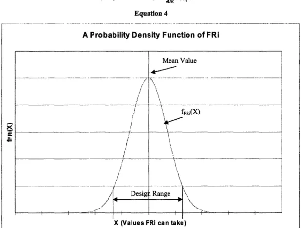
The complexity of a design is measured in the uncertainty of the DPs ability to satisfy the FRs. In a time-invariant design, the uncertainty is the probability that an FR will be successfully fulfilled. This probability is captured by the overlapping of the design range and the system range. The design range is the acceptable range of values in which an FR can reside. The system range is the range of values in which the FR actually resides. For example, suppose that a FR is satisfied on the design range of 0.125. +/- 0.03125 and the FR actually remains uniformly distributed on the system range of 0.109375+!- 0.015625. This system range is entirely within the design range, and therefore that FR has a 100% probability of success. Suppose that, instead, the FR's system range was 0.25 +/- 0.125 with uniform probability. This determines that the probability of success of that DP satisfying that FR is 0.03125/0.25 or 12.5%.
In general, the design range is the acceptable range of values that an FR can take, and the
density function, seen in Figure 3. The probability of success is the area underneath the curve of the probability density function,fFR, of the FR on the design range (DR). This relationship is captured in Equation 4.
P(FR Successful) = R fFR, (x)dx
Equation 4
X
A Probability Density Function of FRI
Mean ValueDesign Range
X (Values FRi can take)
Figure 3: Probability Density Function of FR
The uncertainty can also be represented in another way, called information. The information of the uncoupled FRi is defined in terms of the probability Pi of Satisfying FRi, as seen in Equation 5.5
I, =-log2 i
Equation 5
The information axiom states that the designer should minimize the information content of the design. The best design therefore is the one with the least information content, or in other words, the best design is one that has the highest probability of satisfying all the FRs. Information content, therefore, becomes a useful measurement of the complexity of a system, which can also be defined in terms of uncertainty of being able to fulfill all the FRs of the system.
Thus, the design information is completely captured in the Axiomatic Design framework, from the customer needs domain, to the functional and physical domains. The complexity of the design is captured by the uncertainty in fulfilling all the FRs.
Connecting Design and Cost Information
In order to connect the design description of the system with cost information, another domain is created. This new domain is termed as the costing unit domain. The costing units (CUs) are physical entities that represent the actual system. To some degree, it is equivalent to the bill of materials (BOM), list of components, or work breakdown structure (WBS). CUs are not the same as DPs, since DPs can be variables or characteristics that are not necessarily physical parts. For example, a beverage can has 12 FRs and 12 corresponding DPs, but only three CUs - integrated physical components. The design of the main body of the can should satisfy the FRs of containing radial and axial pressure and withstanding impact from a 2m height by modifying DPs like the material, thickness, radius, length, and convex shape of the bottom of the can.6 In our model, FRs, driven by customer needs, are mapped into DPs, and DPs are mapped into CUs. This chain of information enables us to assess the impact of the FRs on cost. Thus, information that historically has resided in two separate domains is now integrated together, as seen in Figure 4.
Functional Physical Cost
Domain Domain Domain
FRI DPI
I-i-I$
ull.
C ,$ -CU12, $
FRI1 FR12 DPI DPI
CU13 $
FR11i HR1 F.121 FR122 DP 11
~
t D PFR11M M2 R1211 R121 OP11 DP11 MP2 DPI2 U2$
Figure 4: FRs and DPs are connected to CUs, naturally linking design and cost information together. The FR-DP structure in our model is hierarchical. As the design matures from conceptual solutions to detailed solutions, the FR-DP map develops deeper levels of hierarchical structure. Since the cost information is closely tied to the FR-DP map in our model, it naturally produces a system design cost breakdown from the top-level to leaf-levels. This cost breakdown, along with the hierarchical design description, offers a good way to manage cost information. In the next chapter, one example of the utility of this link will be shown. The framework will be used to track the propagation of a design change to a functional requirement into the cost domain.
Traceability
Traceability is being able to track the relationship between requirements and the solutions that satisfy those requirements. How does Axiomatic design aid in traceability? Refer to Figure 5 and Figure 6. Notice that the design parameter, DP121 affects FR121, FR122, and FR123.
Suppose that we need to determine the impact of a requirement change to FRI21. In order to satisfy the change in that requirement, DP 121 will have to be changed. Because DP 121 affects FR122 and FR123, then those requirements may not longer be satisfied after DP121 is changed. This, therefore, implies that DP122 and DP123 must change as well. Note that a change to DP123 will propagate to the lower levels FR1231 and FR1232. Therefore, traceability is obtained by identifying which solutions are likely to change due to a requirement change and then see what 6
other requirements may be affected. The design matrix provides an easy way to determine which requirements and design solutions will be affected by a change.
Figure 5: A Requirement and Solution Decomposition
FRI FRFO I MPDPI,0 A~F1 FR1 I OR3F R27 I F F I 0 F R0 000 O JO * 00. Ft: FR1.:F -FR11:FR1 o o o oo o o3 FR1 .22: FR2 2 FR .2.3: FR123 o . 0 0 0 o -FR.2..: FR123 00 0 0 0 0 0 -FR1.2.3:FR123 o 0 0 & 0 9-FR2:FR2 00000000O O FR2.1: FR21 00 M000 0 0 0 FR2.2:FR22 0 0 0 0 0 0 0 0 0 0 FR2.:FR23 ooooo 0 Q 0
Figure 6: A matrix highlighting the relationship between solutions and requirements. The current process of capturing traceability in the industry lacks DPs and their
relationship to requirements. Instead only requirements and their related hierarchy are captured. Suppose that a design had the same situation as described by Figure 5. Following the industry's
SR I SR 2
SR1
F
SR2
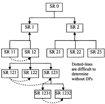
SR 11 SRI12 SR 21 SR 22 SR 23 Dotted-lines are difficult to SR 121 SR 122 SR 123 determine without DPs SR 1231 SR 123Figure 7: A hierarchial system requirement (SR) decomposition of the same design as in the previous two Figures.
In order to provide an adequate amount of traceability (the same as provided when design parameters are used), SR 11 should link to SR 12, SR 121 should link to SR 122 and 123, and SR 1231 should link to SR 1232. These links are represented by the dotted-lines in Figure 7. This would provide the same result as that from the previous two figures. The way that these links are typically determined is through design parameters. So whether or not design parameters are recorded, the links are established by design parameters. There would be no other way to determine how two seemingly unrelated system requirements are related. It is only by determining an intermediate parameter that affects whether both requirements are satisfied. Design parameters are inherently in the design process, but are typically not recorded and related to functional requirements. Axiomatic design requires the designer to record design parameters and their relation to requirements. Traceability, therefore, is inherent in the Axiomatic design process.
The credibility of a cost estimate is enhanced by traceability because it provides
additional information about the design that was not available before. For example, when a design change is introduced, it will become immediately apparent which functional requirements, design parameters, and costing units are involved in that change. This helps to define what the scope of the design change should be. When a design change is introduced, without traceability it is difficult to determine which costing units will be affected. As a result, the actual list of costing units that will be affected by a change may be different from what is identified and, therefore, the scope of the design change could be incorrect. A cost estimate based on an incorrect scope, no matter how accurate the cost estimating tools used, will still be incorrect. The next chapter shows how traceability is used to define the scope of a design change.
Summary
Current cost estimation practices do not adequately take into account all aspects of the design, including customer needs, functional requirements, design parameters, and complexity. They solely rely on physical parameters of a design like weight, power, number of gear teeth, etc to determine cost information. Historical data attempts to fill in the gap by taking into account
past trends in design complexity and iteration. Our model enhances the credibility of cost estimation by linking design and cost information together.
The axiomatic design framework provides a good description of the design. It maps the customer needs into functional requirements (FRs), and then to design parameters (DPs). The relationship between FRs and DPs is represented by the design matrix. The design matrix is essential in revealing the complexity of the design, which is defined as the uncertainty in fulfilling all the FRs. This uncertainty is measured in terms of the overlap of the design and system ranges. The design matrix also uncovers the coupled nature of the design. This coupling can either be eliminated through developing a better design or can be dealt with properly by varying the DPs in the correct sequence or through design iteration. When used correctly, axiomatic design becomes a great tool to aid in the designing process and results in a solid description of the design.
Design and cost information are linked together by linking the FR and DP domains to a new costing unit domain. A costing unit (CU) can be thought of as a component of the Work Breakdown Structure (WBS) and is the typical object of the cost estimation efforts. The link occurs by mapping DPs to the respective CUs. Since the cost information is closely tied to the FR-DP map, it naturally produces a system design cost breakdown from the top-level to leaf-levels. The utility of this link is shown in the following chapter in determining the cost of a design change.
Traceability is being able to track the relationship between requirements and the solutions that satisfy those requirements. The axiomatic design process requires the designer to record all the design solutions and their relation to FRs. By doing so, the designer is inherently increasing the traceability in the design. Traceability aids in defining the scope of a design change. Without traceability, a team of experts must come together and try to identify the requirements and solutions that will be affected by the change. The team of experts can potentially include unaffected requirements and solutions and exclude others that are affected. The result is that the scope of the cost estimate is erroneous. With traceability, it immediately becomes apparent which FRs, DPs and CUs will be affected by the design change. The scope of the design change is clearly and correctly defined, adding credibility to the cost estimate.
Chapter 3
Quickly Estimating the Cost Impact of a Design Change
to Development
How does a design change affect the life-cycle cost of a system? First of all, it will help to define what a design change is. A design change is usually implemented by a designer either because the customer needs or constraints have changed, or because the functional requirements (FRs) directly have been changed. Design parameters (DPs) are then modified in order to meet the changed FRs. Also, technical advances or roadblocks may encourage the use of a different DP. The general procedure in determining the cost impact of a design change should start with
determining which DPs must change. Then a magnitude of the change to each DP should be determined. This magnitude should then translate into an increase or decrease in life-cycle cost.
This chapter focuses on determining the cost impact of a design change to the
development cost. The general method of determining the cost impact of a design change applies here. A set of FRs are identified as changed, thereby requiring certain DPs change. The set of DPs that must change are determined from the design matrix. Now, in order to estimate the
development cost, the affected components, or CUs, are identified by a DP-CU, and CU-CU matrix and the time required to complete the design changes for each component is determined using a Task-based model. This procedure takes into account the physical interactions between components, in order to determine how the change propagates through the system. The additional iterations required to make the change are determined by a Task-based model, which quantifies the coupling of tasks. Once the additional time required to finish each component after a design change is determined, the time directly translates into labor costs. Historically, the development labor cost is approximately directly proportional to the total development cost, which includes material and labor costs. The total development cost due to the design change, then, is estimated.
Once the model is constructed, all that is required is the input of several parameters in order to determine the cost impact of a design change. This model once encoded into software, therefore, is an extremely quick and useful tool that aids in the management process as design changes are being considered for implementation. Typically, it takes organizations several weeks to determine what the actual impact of a design change will be to the design and life-cycle cost. Their analysis is not always guaranteed to be complete either. Instead, this model outputs the affected components, how they are affected, and what the cost impact will be. The output from this model also serves as a medium of discussion about design changes for organizations like Ingall's and the US Navy. The implications of this model, therefore, are of interest to not only cost estimators, but to the system-developing organization as a whole.
Identify the Components Affected by a Functional Change
The Axiomatic design framework provides a mapping from customer needs into FRs, or the set of functions that the product must perform in order to satisfy the needs of the customer. FRs are then mapped into DPs, or specific engineering parameters that are varied in order to perform the desired functions.7 By doing this, a clear connection is established between the
customer's needs and the actual product being designed. The relationship between FRs and DPs, as seen in Figure 8, is of special interest. There are three FRs and three DPs that are related to each other by this matrix. FRI is affected by DP1, FR2 is affected by DP2 and FR3 is affected by DP2 and DP3. Or in other words, if DPI is changed, FRI will be affected, if DP2 is changed, FR2 and FR3 will be affected, and if DP3 is changed, FR3 will be affected. Later, this
information will be used to identify which DPs will be necessary to change in order to satisfy a change to a functional requirement.
DPI DP2 DP3
FR1 X
FR2 J
FR3 X X
Figure 8: The FR-DP Relationship
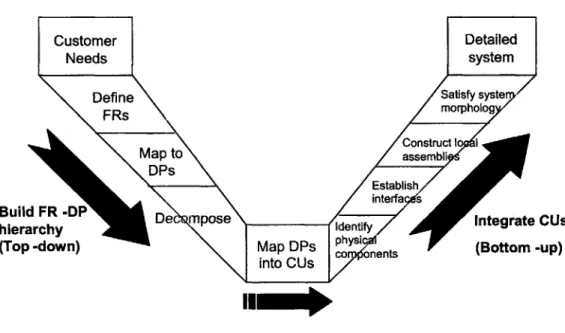
The V-model, shown in Figure 9, illustrates how the design process works. The left-hand part of the V shows the top-down axiomatic design approach, which was described at length in Chapter 2. FRs are developed from customer needs. DPs are then created that can satisfy those FRs. The decomposition process unravels more details of the design. Once this process is completed, all the physical components, or costing units (CUs), must be identified. CUs are the objects of the cost estimation, and the physical artifacts generated from the design. For the beverage can, the three physical components of the can would be the three CUs. Each DP can be embedded in multiple CUs and each CU can embody multiple DPs. The reason one DP can map to several CUs originates from the fact that designers create CUs that are at a lower level than the available DPs. For example, one FR may state "Provide fuel to the engine" and the corresponding DP would be a Fuel Delivery System. This may include CUs such as a fuel tank, fuel pump, fuel lines. This higher level DP would correspond to these three CUs in the absence of further decomposition. After full decomposition, this problem will no longer occur. The relationship between DPs and CUs can be seen in the example in Figure 10. CUI contains DPI and DP2; CU2 contains DPI, DP2 and DP3; CU3 contains only DP4. Finally, once all CUs have been identified, these CUs must be integrated into a complete system.
Customer Detailed
Needs system
Define Satisfy syste
F~s morpholog Construct I I Map to assembli D~s Establish/ interfa s
Build FR -DP Dec mpose ntegrate CUs
hierarch dni
(Top -down) Map DPs physi (Bottom -up)
into CUs co net IINM
cul
DP1 X DP2 DP3 DP4 CU2 CU3 X X X X XFigure 10: The DP-CU Relationship
With the FR-DP and DP-CU matrices, we can determine the list of components that are affected by a functional change. Suppose that the following design matrix, in Figure 11, was
under consideration for a significant design change. In order to best satisfy the customer needs, a
manager decides that FRI will have to change. Consequently, in order to satisfy FRI, DPi will
also have to change. Because DP 1 also affects FR6, DP6 will have to be changed in order to
compensate for the change in DP 1 and still satisfy FR6. The result of the change to FRI is that DPI and DP6 will have to change.
FR change Off-diagonal ter Indicates FR6 is affected by DPi 'FRi FR2 FR6 FR9 m change x x x rX X xX X X 1X X* X X X X X X LM: X X X
DPI
DP2 DP6 DP9 DP6 to respond FR6 effectFigure 11: A change to FRI requires a change in DP1 and DP6
From the DP-CU relationship, seen in Figure 12, we can find the CUs (components) that will be affected by the changes to DPI and DP6. Reading from left to right and then up, we can identify CUl and CU3 as the components that will need to be changed as a result of the change to FRI. Thus the output from the DP-CU matrix is a list of components affected by the functional
changes.
Development CUi CU2 CU3
DP2
DP2
DP6 4FIX
0
x
x
x
DPn 0 X 0I
.--
a
Figure 12: A change in DP1 and DP6 necessitates a change in CU1 and CU3.
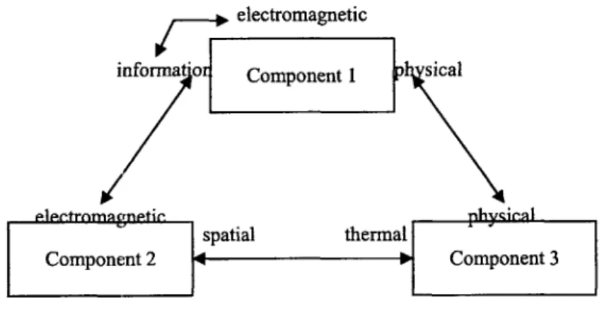
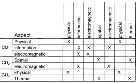
This list of affected components only takes into account functional interactions between DPs. Many components interact with each other physically as well as functionally. However, this information is typically not captured by a design matrix. Instead, a new CU-CU matrix was created in order to capture physical interactions between CUs. Imagine a set of components that physically interact with each other, as in Figure 13. Five examples of component attributes that can interact with other components are physical, spatial, thermal, information and
electromagnetic. The physical attribute indicates that this component physically integrates with another component, for example, by a mount or tubing. The spatial attribute specifies size or location of the component. The thermal attribute marks the presence of heat exchange or
generation. The information attribute is the flow of information into and out of a component. The electromagnetic attribute is the transmission of an electromagnetic signal into or out of a
component. A component can interact with its neighbors through any combination these five attributes. For example, In Figure 13, the physical attribute of Component 1 interacts with the physical attribute of Component 3 and the information attribute of Component 1 interacts with the electromagnetic attribute of Component 2. These interactions are two way because of the question that we ask: "Does the information attribute of Component 1 interact with the electromagnetic attribute of Component 2?" "Does the electromagnetic attribute of Component 2 interact with the information attribute of Component 1?" is the same question. The answer is yes for both
questions, since they are the same question. Even an attribute within component I could interact with another attribute of component 1. In the example in Figure 13, the information and
electromagnetic aspects of component 1 interact with each other.
f-*
electromagneticinformat'o Component 1 p sical
IlCmmnti spatial thermal ysr
Component 2 4Component 3
Figure 13: Component Interactions
Unfortunately, diagrams like this become difficult to create and read as the number of components or CUs increases to the hundreds, or even thousands. A CU-CU matrix better captures this information. Essentially, the CU-CU matrix is a collection of two-way pointers that
connect the CU attributes. By definition, this matrix is symmetric. The equivalent matrix of Figure 13 can be seen in Figure 14. This matrix is also similar to that of a component design
structure matrix.
Ctcu,
CU
2CU
a)) 0 CU C -~~ E E -0~E 2 - 0 o CU F >1 0 M5 U 1
Aspect
a
a) 0C_ Physical X X CU1 information X X X electromagnetic X X CU2 Spatial X X electromagnetic X X CU3 Physical XX
Thermal X XFigure 14: The CU-CU Matrix
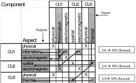
By using a CU-CU matrix, the list of affected CUs from a functional change can be
refined and expanded. The following example will demonstrate the propagation of changes through interfaces of components. Recall from Figure 12 that CUl and CU3 had been identified as the affected CUs by a functional change in FRI. Suppose that the interactions between the three CUs were characterized by the CU-CU matrix in Figure 14. Certain attributes of CUl and
CU3 will change to satisfy the FRs that had been changed. Suppose that the information attribute
of CUI and the thermal attribute of CU3 were changed. This type of change would necessitate a change in the electromagnetic attribute of CUI and the spatial and electromagnetic attributes of
CU2. The interface between the information and electromagnetic attributes of CUl is represented by the two X's at (2,3) and (3,2). Because this interface was identified as necessary to change,
both X's are marked. The method of determining the affected interfaces is known as change propagation outlined in Figure 15. All the X's in the column of a changed attribute are marked as necessary to change. For example, following the line from the thermal attribute of CU3 identifies the spatial attribute of CU2 as being affected. The input to the CU-CU matrix is the information attribute of CU 1 and thermal attribute of CU3 and the output is the information and
electromagnetic attributes of CU I, the spatial and electromagnetic attributes of CU2, and the thermal attribute of CU3. This successfully identifies the complete list of affected CUs and even the attributes and interfaces of the CUs that will be affected by the change. This step can be repeated with the output as input in order to reflect further propagation of the change.
Componert
CIA
CU2
CU3
.2o Inputs
Outputs E E
CU1
xoai3/
0
Rework
CU2_/4+
0
X
X__
0%Rwork0)3
physical
CU eme=
x
X
2/4+ 50% Rework
Figure 15: Determining the complete list of CUs affected by a functional change by analyzing the interactions between CUs.
The nature of propagation of a change can be understood better through an example.
Suppose that in the middle of the design of a car, it is decided that the size of the trunk must
change. The trunk is connected to the frame of the car, and therefore, a change in the size of the
trunk could affect the design of the frame. The frame of the car is also connected to the engine bay, and if the frame design changes, then perhaps the engine bay design must also change. If the
engine bay design changes, perhaps the engine, intake, headers, or throttle body may have to change. This question could continue until all components had been identified as affected due to a change in the trunk. This is not very useful for cost estimation analysis. Instead, the "nearest neighbor" rule is employed. The nearest neighbor rule states that a change to a component only propagates changes to components that are directly connected to that component. For the CU-CU
matrix, this means that the process of change propagation is only performed once.
A measure of the magnitude of a change is the number of affected interfaces or attributes
out of the total number of interfaces and attributes. Note that interfaces are indicated by
off-diagonal X's, while off-diagonal X's indicate attributes in a CU-CU matrix. We later use this
measurement to determine the amount of rework that must be done to complete the design change. The calculation of percentage rework can be seen in Equation 6.
% Rework = # of Affected Interfaces or Attributes
Total # of Interfaces and Attributes Equation 6
Take, for example, CU 1 from Figure 15 and calculate the % Rework. There are three attributes and three interfaces, for a total of six interfaces and attributes. The information attribute will
have to change and the CUl Information - CUl Electromagnetic, and CUI Information - CU2
Electromagnetic interfaces will have to change, for a total of 3 affected interfaces and attributes. The % Rework is then calculated to be 3/6, or 50%. This indicates that 50% of the CUl design
must be redone, while the other 50% can still be used.
8 The X's at (3,2) and (2,3) count as one interface within CU 1.
I
Determine the Development Labor Cost
Now that the complete list of CUs has been identified and the amount of rework required for each CU has been calculated, the amount of development time required to implement those changes can be determined. By measuring the impact of a change on the development time of a project, the cost of labor can be determined. This is accomplished using a task based model.9 Recall from Equation 2 that the total development cost is the sum of the labor and material costs accrued during the development phase. This section is specifically dealing with the labor portion.
The task based model is a record of the interaction between all the processes in a project and a means of calculating the time required to complete each task. There are three different configurations of two tasks A and B, as seen in Figure 16. If task B requires information from task A, the task A must be completed before task B. These two tasks are sequenced in series. If tasks A and B do not require information from each other, then they can be performed in parallel.
If tasks A and B require information from each other, then they have to be performed in parallel
with iterations involved. We chose to model tasks as being done all at the same time (in parallel), though development typically involves a mixture of the three forms of task sequencing.
AA
BB
Dependent Tasks Independent Tasks Interdependent Tasks
(Series) (Parallel) (Coupled)
Figure 16: Three possible sequences for two tasks.'0
Drawing figures aids in the visualization of how tasks interact, but this practice becomes less useful and more cumbersome as the number of tasks increases. The work transformation matrix, WT, is used instead, as seen in Figure 17. This matrix shows that tasks A and B are coupled, interdependent tasks. In a parallel iteration model, tasks run through an iteration, and then exchange information, thereby creating additional work called rework. Both tasks iterate in this way until both tasks are completed. The total time in order to complete each task, therefore, is the sum of the time spent on each iteration. The values in the matrix represent the percentage of rework created at the end of each iteration. The work transformation matrix in Figure 17 indicates that task B creates an additional 50% of rework for task A and that task A creates an additional
30% rework for task B after each exchange of information.
AB
Figure 17: A Work Transformation Matrix, WT, with Two Coupled Tasks
Mathematically, the total time required to complete two tasks in parallel is the following. The initial work vector, uO, represents the initial amount of work required to complete each task
9 See reference [3] and [4].