HAL Id: hal-00296118
https://hal.archives-ouvertes.fr/hal-00296118
Submitted on 23 Jan 2007
HAL is a multi-disciplinary open access
archive for the deposit and dissemination of
sci-entific research documents, whether they are
pub-lished or not. The documents may come from
teaching and research institutions in France or
abroad, or from public or private research centers.
L’archive ouverte pluridisciplinaire HAL, est
destinée au dépôt et à la diffusion de documents
scientifiques de niveau recherche, publiés ou non,
émanant des établissements d’enseignement et de
recherche français ou étrangers, des laboratoires
publics ou privés.
patterns of volatile organic compounds in the Valley of
Mexico during the MCMA 2002 & 2003 field campaigns
E. Velasco, B. Lamb, H. Westberg, E. Allwine, G. Sosa, J. L. Arriaga-Colina,
B. T. Jobson, M. L. Alexander, P. Prazeller, W. B. Knighton, et al.
To cite this version:
E. Velasco, B. Lamb, H. Westberg, E. Allwine, G. Sosa, et al.. Distribution, magnitudes, reactivities,
ratios and diurnal patterns of volatile organic compounds in the Valley of Mexico during the MCMA
2002 & 2003 field campaigns. Atmospheric Chemistry and Physics, European Geosciences Union,
2007, 7 (2), pp.329-353. �hal-00296118�
www.atmos-chem-phys.net/7/329/2007/ © Author(s) 2007. This work is licensed under a Creative Commons License.
Chemistry
and Physics
Distribution, magnitudes, reactivities, ratios and diurnal patterns of
volatile organic compounds in the Valley of Mexico during the
MCMA 2002 & 2003 field campaigns
E. Velasco1,*, B. Lamb1, H. Westberg1, E. Allwine1, G. Sosa2, J. L. Arriaga-Colina2, B. T. Jobson3,**, M. L. Alexander3, P. Prazeller3, W. B. Knighton4, T. M. Rogers4, M. Grutter5, S. C. Herndon6, C. E. Kolb6, M. Zavala7, B. de Foy7,*, R. Volkamer8, L. T. Molina7,*, and M. J. Molina8
1Laboratory for Atmospheric Research, Department of Civil and Environmental Engineering, Washington State University,
Pullman WA, USA
2Laboratorio de Qu´ımica de la Atm´osfera, Instituto Mexicano del Petr´oleo, M´exico D.F., M´exico 3Atmospheric Sciences. Battelle Pacific Northwest National Laboratory, Richland WA, USA 4Department of Chemistry and Biochemistry, Montana State University, Bozeman MO, USA
5Centro de Ciencias de la Atm´osfera, Universidad Nacional Aut´onoma de M´exico, M´exico D.F., M´exico 6Center for Atmospheric and Environmental Chemistry, Aerodyne Research Inc., Billerica, MA, USA
7Department of Earth, Atmospheric, and Planetary Sciences, Massachusetts Institute of Technology, Cambridge MA, USA 8Department of Chemistry and Biochemistry, University of California, San Diego, USA
*now at: Molina Center for Energy and the Environment (mce2.org), La Jolla CA, USA **now at: Washington State University, Pullman WA, USA
Received: 7 July 2006 – Published in Atmos. Chem. Phys. Discuss.: 8 August 2006 Revised: 21 December 2006 – Accepted: 12 January 2007 – Published: 23 January 2007
Abstract. A wide array of volatile organic compound (VOC)
measurements was conducted in the Valley of Mexico dur-ing the MCMA-2002 and 2003 field campaigns. Study sites included locations in the urban core, in a heavily industrial area and at boundary sites in rural landscapes. In addition, a novel mobile-laboratory-based conditional sampling method was used to collect samples dominated by fresh on-road ve-hicle exhaust to identify those VOCs whose ambient con-centrations were primarily due to vehicle emissions. Four distinct analytical techniques were used: whole air canister samples with Gas Chromatography/Flame Ionization Detec-tion (GC-FID), on-line chemical ionizaDetec-tion using a Proton Transfer Reaction Mass Spectrometer (PTR-MS), continu-ous real-time detection of olefins using a Fast Olefin Sensor (FOS), and long path measurements using UV Differential Optical Absorption Spectrometers (DOAS). The simultane-ous use of these techniques provided a wide range of indi-vidual VOC measurements with different spatial and tempo-ral scales. The VOC data were analyzed to understand con-centration and spatial distributions, diurnal patterns, origin and reactivity in the atmosphere of Mexico City. The VOC
Correspondence to: E. Velasco
(evelasco@mce2.org)
burden (in ppbC) was dominated by alkanes (60%), followed by aromatics (15%) and olefins (5%). The remaining 20% was a mix of alkynes, halogenated hydrocarbons, oxygenated species (esters, ethers, etc.) and other unidentified VOCs. However, in terms of ozone production, olefins were the most relevant hydrocarbons. Elevated levels of toxic hydrocar-bons, such as 1,3-butadiene, benzene, toluene and xylenes, were also observed. Results from these various analytical techniques showed that vehicle exhaust is the main source of VOCs in Mexico City and that diurnal patterns depend on vehicular traffic in addition to meteorological processes. Fi-nally, examination of the VOC data in terms of lumped mod-eling VOC classes and its comparison to the VOC lumped emissions reported in other photochemical air quality mod-eling studies suggests that some alkanes are underestimated in the emissions inventory, while some olefins and aromatics are overestimated.
1 Introduction
Volatile organic compounds (VOCs) play a key role in pho-tochemical air quality in urban atmospheres. In the pres-ence of sunlight and nitrogen oxides (NOx), VOCs
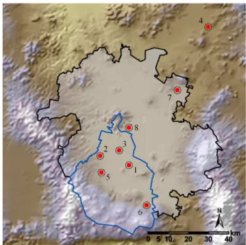
oxida-Fig. 1. Sampling sites during MCMA-2002 and MCMA-2003 field campaigns. Points indicate the location of the sampling sites and numbers correspond to the sites listed in Table 1. The shadow limited by the black contour represents the boundary of the called “Mexico City Metropolitan Area”, while the blue contour limits the Federal District. The Mexico City Metropolitan Area is more a po-litical name than a topographic denomination to identify the exten-sion of Mexico City.
tion produces secondary products including radicals (e.g., hydroxyl, hydroperoxy, organoperoxy), oxygenated organ-ics (e.g., aldehydes, ketones, acids, nitrates, peroxides), and inorganics (e.g., carbon monoxide, ozone, hydrogen perox-ide, nitric acid) (Finlayson-Pitts and Pitts, 1997). It has been demonstrated that many of these secondary compounds may have direct health impacts (Evans et al., 2002, and references therein), and that some individual VOCs are extremely toxic pollutants (e.g., the carcinogens benzene and 1-3-butadiene). Mexico City with a population of 19 million is a good ex-ample of a megacity with severe air pollution problems. It is situated in the Valley of Mexico and is the capital city of a developing country. Mexico City is in the subtropical zone and at high altitude which makes combustion processes less efficient, leading to enhanced VOC emissions. Mexico City’s high altitude (∼2240 m) and low latitude (19◦25′N), result in subtropical weather and intense solar radiation that accentuate the VOC evaporative emissions from a variety of sources such as storage and distribution of gasoline, solvent-base cleaning, painting, and industrial processes. However, the main contributors to high VOC concentrations in Mex-ico City are the extensive presence of aged industrial opera-tions (more than 53 000 industries) and a relatively old vehi-cle fleet (more than 3.5 million vehivehi-cles with an average age
of ∼9 years). The elevated anthropogenic emissions, the in-tense solar radiation and area’s topography with mountains to the west, east and south of the valley (see Fig. 1) produce elevated levels of photochemical pollutants on a daily basis (Molina and Molina, 2002).
Many researchers have addressed the VOC pollution prob-lem in Mexico City. Ambient VOC concentrations have been evaluated since the early 90’s (Raga et al., 2001 and refer-ences therein). All of these studies have consistently reported high concentrations of propane, butane and other low molec-ular weight alkanes, which have been attributed to liquefied petroleum gas (LPG) leakage during handling, distribution and storage. LPG is the main fuel for cooking and water heat-ing in Mexican households. High ambient concentrations of photochemical reactive VOCs, such as olefins and aromatics, have been reported as well (Mugica et al., 2002a; Arriaga et al. 1997). These two VOC groups have been identified as the main species responsible for the ozone and secondary or-ganic aerosol (SOA) formation in Mexico City (Gasca et al., 2004; Mugica et al., 2002a). High levels of aromatic hydro-carbons, particularly of toluene, benzene and xylenes, have been detected in different microenvironments and associated with diverse public transport systems in Mexico City (Shio-hara et al., 2005; Gomez-Perales et al., 2004; Cruz-Nu˜nez et al., 2003; Bravo et al., 2002; Ortiz et al., 2002; Meneses et al., 1999).
From source apportionment studies, it has been deter-mined that motor-vehicles, especially gasoline-powered ve-hicles, are the main source of aromatic hydrocarbons (Mug-ica et al., 2003). Emissions profiles for on-road motor-vehicles have been obtained from tunnel studies (Mugica et al., 1998). Schifter et al. (2003) estimated on-road emis-sions of total hydrocarbons using remote sensors, and re-cently Zavala et al. (2006) and Rogers et al. (2006) quan-tified mobile emissions of benzene, toluene, formaldehyde and acetaldehyde via mobile laboratory “chase” experiments for real on-road conditions. However, vehicular emissions in Mexico City are still uncertain due to the lack of reliable fleet emission factors and daily activity levels (Gakenheimer et al., 2002). VOC emission profiles are also available for food cooking, asphalt application and painting operations, among other types of sources in Mexico City (Vega et al., 2000; Mugica et al. 2001a). The biogenic component in the VOC emission burden has been estimated to contribute no more than 7% in the Valley of Mexico (Velasco, 2003).
During the last decade, a number of policies and actions have been enacted to decrease VOC emissions in Mexico City, among them, the installation of vapor recovery sys-tems in fuel service stations, the banning of heavy fuel oil, the phasing out of leaded gasoline, the availability of diesel with reduced sulfur content and the substantial reduction of olefins, as well as benzene and other aromatic hydrocarbon content in gasoline. Arriaga-Colina et al. (2004) reported that, as result of these emission control measures, ambient VOC concentrations have stabilized and possibly decreased
in the last 10 years, despite the growth in the vehicular fleet and other activities. However, ambient VOC levels still re-main high and contribute to the exceedences of the national air quality standard for ozone on 70% of the days each year (110 ppb/1 h average; GDF, 2004).
Although some advances have been achieved, it is clear that a better understanding of photochemical pollution in the complex urban ecosystem of Mexico City is needed to sup-port effective air quality emission control strategies. In this context, a number of US and Mexican institutions and agen-cies participated in the Mexico City Metropolitan Area 2002 and 2003 (MCMA-2002 & MCMA-2003) field campaigns. MCMA-2002 was an exploratory campaign performed in February 2002, and MCMA-2003 was an intensive five-week field study during April and May, 2003. The goals of both field studies were to update and improve the emissions in-ventory of Mexico City, and to gain a better understanding of the chemistry and transport processes driving atmospheric pollution in the valley. As part of the effort to meet these goals, a wide array of VOC measurements was conducted at airshed boundary sites, central urban core sites, and down-wind urban receptor sites. Four different analytical methods were used: VOC speciation by Gas Chromatographic anal-ysis using Flame Ionization Detection (GC-FID), olefin de-tection with a Fast Olefin Sensor (FOS), determination of a number of oxygenated and aromatic VOCs by Proton Reac-tion Transfer Mass Spectroscopy (PTR-MS), and measure-ments of selected VOCs using Differential Optical Absorp-tion Spectroscopy (DOAS). Key aspects of these VOC surements were the large number of individual species mea-sured under a variety of spatial and temporal scales employed in the measurements.
This manuscript presents a summary of results from the different VOC measurements in terms of the distribution, magnitudes, and diurnal patterns of selected VOCs. Ratios of individual VOC species are used to characterize different sites, to investigate the relative reactivity of different species and to determine their origins through comparisons with source signatures, in particular with vehicle exhaust profiles. In addition, the ambient VOC data have been compared to the lumped VOC emissions classes reported by West et al. (2004) to model the photochemical processes in the atmosphere of Mexico City. It has been suggested that VOC emissions are underestimated in the official emissions inventory by a factor of 3 from analysis of the VOC/NOxratio (Arriaga-Colina et
al., 2004) and from ozone modeling exercises (West et al., 2004). However, eddy covariance flux measurements of se-lected VOCs during the MCMA-2003 campaign suggest that for the VOC classes measured, the VOC emissions reported in the emissions inventory are generally correct (Velasco et al., 2005).
2 Monitoring sites
During the MCMA-2002 study, five sites were selected for measuring ambient VOCs with instantaneous canister sam-ples. For the MCMA-2003 study, two 2002 sites were ex-cluded and three new sites were added, and diverse mea-surement techniques were implemented. Figure 1 shows a map of the Valley of Mexico indicating the monitoring sites where VOC measurements were performed in both cam-paigns. Overall, eight sites were employed; four locations were urban sites with different mixtures of commercial, res-idential, and light industrial activity (La Merced, Consti-tuyentes, Pedregal and CENICA), one location was in an industrial section of the city (Xalostoc), and three locations were boundary sites in rural areas (La Reforma, Teotihua-can and Santa Ana Tlacotenco). Table 1 lists a summary of these sites and VOC measurement techniques used during the MCMA-2002 and MCMA-2003 field campaigns.
3 Instrumentation
3.1 Gas chromatography separation and flame ionization detection (GC-FID)
Ambient VOC samples were collected from all monitoring sites in Summa® electro-polished stainless-steel canisters. During the MCMA-2002 study, 46 samples were filled in-stantaneously, while for the MCMA-2003 study, 184 sam-ples were collected in periods of 30 min, 1 and 3 h using au-tomated samplers. The different duration of the sampling periods was due to the specific sampling objectives at each site. From both studies, 64% of the samples were collected during the morning rush traffic period (6:00 to 9:00 h) when VOC concentrations are strongly related to traffic emissions and before photochemical processing has started. The re-maining samples were collected during the late morning and early afternoon hours.
Canister samples were collected and analyzed by two dif-ferent research groups: Washington State University (WSU) and the Mexican Petroleum Institute (IMP). WSU collected and analyzed 78% of the samples. During the MCMA-2003 study, WSU collected all its samples with a XonTech, Inc. Air Sampler model 910PC. Half of the samples were ana-lyzed on-site within 24 h of collection; the remainder ples were returned to WSU for analysis. IMP collected sam-ples only in 2003 using an AVOCS Anderson Automated Sampler with a Viton diaphragm pump. Both groups an-alyzed their samples using methodology similar to the US EPA compendium methods TO-14/15 (USEPA, 1999a). The GC analysis utilized cryogenic pre-concentration by drawing air from the canisters through a stainless-steel loop contain-ing glass beads (60/80 mesh) and cooled to liquid oxygen temperature. WSU employed a Hewlett-Packard 6890 Series chromatograph. The GC was equipped with a 30-m fused
Table 1. Description of the VOC monitoring sites during the MCMA-2002 (7–24 February) and 2003 (1 April–5 May) field campaigns. The numbers in parenthesis in the column of methods indicate the number of collected samples in canisters or the number of days monitored by PTR-MS, DOAS or FOS.
Site # Site and position Year Site description Method
1 CENICA
(N19.358◦, W99.073◦)
2003 MCMA-2003 super site located in the Autonomous Metropolitan University campus Iztapalapa at the southeast of the city in a mixed area with residences, light and medium industries, services and commerce. The traffic is heavy and composed by old and new ve-hicles on paved roads.
Canister sampling and GC-FID analysis (56). PTR-MS (23). FOS (23). DOAS (30). 2 Constituyentes (N19.400◦, W99.210◦)
2002 Western suburban neighborhood close to Chapultepec park.
Heavy traffic on paved roads composed by private cars and heavy-duty diesel buses.
Canister sampling and GC-FID analysis (13).
3 La Merced
(N19.424◦, W99.119◦)
2003 Central city section composed by a mix of residences, small and medium commerce, light industries and a busy market.
Heavy traffic on paved roads with private cars, light-duty vehicles and modern heavy-light-duty diesel buses.
Canister sampling and GC-FID analysis (41). PTR-MS (3). DOAS (30). 4 La Reforma
(N19.976◦, W98.697◦)
2003 Southwestern downwind site from Pachuca, city with 245 000 inhabitants located to the northeast of Mexico City.
Rural site close to urban areas with reduced vehicular traffic on paved and unpaved roads.
Canister sampling and GC-FID analysis (13).
5 Pedregal
(N19.325◦, W99.204)
2002 & 2003 Southwestern suburban neighborhood with paved resi-dential roads lightly traveled.
This site is in the prevailing downwind direction from the center of the city.
Canister sampling and GC-FID analysis (66). PTR-MS (4). 6 Santa Ana Tlacotenco
(N19.177◦, W98.99◦)
2003 Rural site to the southwest of Mexico City, close to the gap in the mountains at Amecameca.
Paved and unpaved roads with minimum traffic.
Canister sampling and GC-FID analysis (13). PTR-MS (3). 7 Teotihucan
(N19.688◦, W98.870◦)
2002 Northern upwind boundary site of Mexico City with pollution influence from a large power plant and large industries around the region.
Canister sampling and GC-FID analysis (7). 8 Xalostoc
(N19.527◦, W99.076◦)
2002 & 2003 North-eastern industrial section of the city with light to medium industries.
Heavy traffic on paved and unpaved roads formed by a mix of new and old gasoline and diesel vehicles.
Canister sampling and GC-FID analysis (21).
silica DB-1 column (0.32 mm i.d. and 1 µm film thickness) with a 2 ml min−1carrier flow. Prior to sample injection, the
oven was cooled to −50◦C. During analysis, the oven tem-perature was raised at 4◦C min−1 to a final temperature of 150◦C. The total analysis time was approximately one hour. Detector response was calibrated with NIST traceable 2,2-dimethylbutane standard. A detection limit of 20 pptC was determined. Individual species were identified by retention times.
IMP conducted their analysis using a Hewlett-Packard 5890 Series II chromatograph containing a 60-m Quadrex fused silica glass capillary column with a phase designation 007 series methyl-silicone (0.32 mm i.d. and coated with a 1 µm film thickness) at a flow of 2 ml min−1. The oven
temperature started at 050◦C and was heated up to 200◦C at a rate of 8◦C min−1. The FID response was calibrated
with a certified high-purity propane standard from Praxair. The detection limit was determined to be 1 ppbC. Individual species were identified by retention times using a mixture of 55 hydrocarbons (Scott Specialty Gases NIST Traceable), and a certified mixture of 33 halogen-containing compounds (Spectra Gases, with 10% analytical accuracy).
3.2 The Proton Transfer Reaction Mass Spectrometry (PTR-MS)
The Proton Transfer Reaction Mass Spectrometry identifies VOCs in ambient air as their molecular mass plus one. This
technique creates ions by transferring a H+from H
3O+ to
the VOCs followed by mass spectroscopy detection of the product ions (Lindinger et al., 1998). The PTR-MS does not employ a column, so response times are short (sec-onds) and automated, continuous measurements can be made over extended periods of time. Specificity in the PTR-MS is achieved by the soft ionization (minimal fragmentation) and the response is limited to species with proton affinity greater than water. In cases where several VOCs produce the same M+1 ion, it is not possible to quantify individual species. For example, the signal at mass 121 (C3-benzenes)
is comprised of i- and n-propylbenzene, three ethyltoluene and three trimethylbenzenes isomers. Validation of PTR-MS measurements have been performed by de Gouw et al. (2003) and Warneke et al. (2003) to determine the set of VOCs that are suitable for measurement with this technique.
During the MCMA-2003 field campaign, two PTR-MS instruments were used. One was operated at the CENICA site by the Pacific Northwest National Laboratory (PNNL), and the second PTR-MS instrument, belonging to Montana State University (MSU), was housed in a mobile laboratory for on-road vehicle emissions studies and both fixed site and mobile ambient pollutant measurements (Kolb et al., 2004; Herndon et al., 2005; Zavala et al., 2006; Rogers et al., 2006). During selected periods, the mobile laboratory was employed as a fixed monitoring station at La Merced, Santa Ana Tlacotenco and Pedregal sites. This manuscript presents only PTR-MS measurements from fixed-sites. The species monitored by PTR-MS included benzene, toluene, styrene, C2-benzenes, C3-benzenes, naphthalene, phenol, cresols,
methanol, acetaldehyde, acetone and acetonitrile. The C2
-benzenes are represented by mass 107, which has contribu-tions from ethylbenzene, o-, m- & p-xylene, and benzalde-hyde (de Gouw et al., 2003).
Both of the PTR-MS instruments were calibrated in the field using a multi-component gas standard containing the species reported here. The calibration standard was diluted with humidified zero air in order to generate a multipoint calibration curve from 1 to 50 ppbv. Calibrations were per-formed every 2–3 days. The instrument background was au-tomatically recorded every 3 h by switching the sample flow to a humid zero air stream. Zero air was continuously gener-ated by passing ambient air through a Pt-catalyst trap hegener-ated to 300◦C. Background count rates were subtracted from the ambient data.
3.3 Fast Olefin Sensor (FOS)
Continuous real-time measurements of olefin concentrations were made at the CENICA site during the MCMA-2003 study by WSU using a FOS. The FOS is a fast isoprene sen-sor (Guenther and Hills, 1998) based on chemiluminescence that occurs when an olefinic bond reacts with ozone. The chemiluminescent response varies considerably for individ-ual olefins. In an urban atmosphere where numerous olefins
are present, it is necessary to evaluate the FOS response to as many olefins as possible. For Mexico City, we determined response characteristics for five olefins (propylene, ethylene, isoprene, 1-butene and 1–3 butadiene). Since NO levels are known to be high in the Mexico City atmosphere, we inves-tigated potential interferences due to its reaction with ozone. Nitric oxide gave no response in this test. Response results for the olefins are shown in Table 2 along with their corre-sponding relative sensitivities to propylene. It was found that the FOS is more sensitive to 1-3-butadiene and isoprene than to propylene; however, their ambient concentrations were much lower than the ambient levels of propylene. In contrast, species with a lower sensitivity than propylene, but with high concentrations in urban atmospheres (e.g., ethylene) can pro-duce large signals.
During the campaign, the FOS was calibrated 3 times per day using dilutions from a propylene standard (Scott Spe-cialty Gases, 10.2 ppm, ±5% certified accuracy). The linear slope of instrument response versus propylene concentration and the zero level exhibited relatively little drift during the study period: 14% and 9%, respectively.
3.4 Differential Optical Absorption Spectroscopy (DOAS) Two research grade, long path DOAS instruments were in-stalled at the CENICA site during the MCMA-2003 study. DOAS is based on the UV-molecular absorption of atmo-spheric gases and measures continuously concentrations of a number of trace gases averaged over a long optical path. In brief, for these two DOAS, light from broadband UV/vis light sources (Xe-short arc lamps) were projected into the open atmosphere onto a distant array of retro reflectors, which folded the light paths back into the instruments where spectra were recorded using Czerny-Turner type spectrom-eters coupled to 1024-element PDA detectors. One DOAS measured formaldehyde and glyoxal, and its results are dis-cussed elsewhere (Volkamer et al., 2005). The second DOAS measured a larger number of VOCs: formaldehyde, ben-zene, toluene, m-xylene, p-xylene, mono-substituted alkyl-benzenes (C2 and higher), phenol, p-cresol, styrene,
naph-thalene and benzaldehyde. These VOCs were measured by observing their unique specific narrow-band (<5 nm) absorption structures through a light path of 430 m (total 860 m) at a height of 16 m. Spectra were recorded by se-quentially observing 40-nm wide wavelength intervals in the wavelength range between 240 and 375 nm at 0.2 nm FWHM spectral resolution. The time resolution of record-ing a full cycle of spectra varied between 30 s and 4 min, depending on the abundance of UV-light absorbing ozone. Absorptions of atmospheric oxygen were eliminated using the interpolation approach of Volkamer et al. (1998), using oxygen column densities of 3.7×10¹⁷molecules cm−2 and 4.1×10¹⁷molecules cm−2, and updated evaluation routines. Reference spectra of aromatic compounds were recorded by introducing quartz-cuvettes filled with vapor into the light
Table 2. Sensitivities, average concentrations measured during selected days throughout the MCMA-2003 campaign between 6 and 10 am by a canister sampling system and GC-FID analysis, FOS responses to those average concentrations, and relative sensitivities to propylene for six compounds.
Compound Sensitivity Average conc., 6–10 am Average FOS response Relative sensitivity (photons ppb−1s−1) (ppb) (photons s−1)c to propylened
Propylene 25.4 7.50 191 1.00 Isoprene 74.7 0.304 23 2.94 Ethylene 17.7 20.7 366 0.70 1-3 butadiene 49.8 0.791 39 1.96 1-butene 7.9 3.90a 31 0.31 NO ∼0.0 61.2b 0 ∼0.0 aAs i-butene
bFrom continuous monitoring during the entire campaign cAverage response = (sensitivity)(average conc.) + (zero value) dRelative sensitivity = (compound sensitivity)/(propylene sensitivity)
beam, and these spectra were calibrated to the absorption cross-sections (Etzkorn et al., 1999). The mean detection limits in ppbv were: 5 (formaldehyde), 1 (benzene, toluene, m-xylene), 0.3 (p-xylene), 1.8 (ethylbenzene-equivalents), 0.5 (styrene), 0.06 (phenol, p-cresol), 0.2 (benzaldehyde), and 0.08 (naphthalene).
Also, during the MCMA-2003 study the National Au-tonomous University of Mexico (UNAM) deployed a com-mercial DOAS system (Opsis, Model AR500) at the La Merced site to measure ambient concentrations of benzene and toluene along a 426-m optical path. The transmitting and receiving telescopes were installed on top of two four-story buildings with the beam trajectory 20 m above the surface. The acquisition time was set to 5 min. Concentrations of ben-zene and toluene were retrieved using the internal evaluation software of the instrument. The instrument response was cor-rected based on a multipoint calibration performed in the lab-oratory and adjusted for real temperature and pressure condi-tions. No humidity correction was applied. Prior to the mea-surements reported here, a reference spectrum (background) was stored for every spectral region used in the analysis us-ing a calibration bench (Opsis CB100, RE060 and CA150) without gas cells installed. A wavelength precision test was also performed using a low-pressure mercury lamp (CA004). More details are provided by Grutter and Flores (2004).
4 Ambient air inter-comparison of GC, PTR-MS and DOAS measurements for selected VOCs
Table 1 shows that at 50% of the monitored sites, two or more different techniques were used to measure VOCs. This pro-vides the opportunity to inter-compare data to verify that they yield consistent results. Figures 2a and b show time series of benzene and toluene mixing ratios measured by GC-FID (WSU), PTR-MS (MSU) and commercial DOAS (UNAM) at
the La Merced site. Both figures show generally good tempo-ral agreement for benzene and toluene. Some differences be-tween concentration levels measured by DOAS and the other two methods are to be expected. The DOAS signal repre-sents average concentrations over an open path distance of about 426 m while the PTR-MS and GC data are from mea-surements at a specific location. The PTR-MS technique is the most sensitive to transient plumes from close-by sources because it measures in real-time with very little temporal av-eraging. This feature can be seen in Fig. 2a where benzene concentrations determined by the PTR-MS are much more variable than those from DOAS or GC-FID. For example the hourly standard deviations of concentrations measured by the PTR-MS are twice those measured by DOAS. Furthermore, it is evident in this figure that the GC results agree better with the PTR-MS than with DOAS which is expected since both GC and PTRMS were point measurements at the same loca-tion.
During the afternoon hours the benzene concentrations measured by DOAS showed a peak that was not registered by the other two techniques. It is unusual to see a benzene peak in the 12–16:00 time period, when atmospheric pho-tochemistry is at its highest rate. Also the relative decrease observed for toluene does not match that of benzene, indicat-ing that the toluene to benzene ratio as calculated from the commercial DOAS data appears to be subject to diurnal vari-ability. It is well known that Opsis DOAS measurements of benzene require an offset correction, which has been applied to the data. The reason for the high benzene values in the afternoon is not easily understood. Kim (2004) and Pinhua et al. (2004) have reported poor correlations between DOAS measurements of benzene and GC-FID measurements for ur-ban environments.
The toluene time series shows better agreement among different techniques and a more normal urban pattern of high nighttime and early morning concentrations and much
Fig. 2. Time series of benzene (a) and toluene (b) mixing ratios measured by DOAS, PTR-MS and GC-FID at the La Merced site. The resolution time for DOAS was 5 min and for PTR-MS ∼30 s. PTR-MS points correspond to 1 min averages. Samples collected by canisters and analyzed by GC-FID correspond to 1 h averages. Short term spikes were commonly observed with PTR-MS indicating local sources.
lower levels during the midday period. Jobson et al. (2007)1 present a more detailed inter-comparison with the same three techniques at the CENICA site. They found that the level of agreement between point and long path techniques is influ-enced by wind direction, but in general terms they also found relatively good agreement between GC, PTR-MS and the re-search grade DOAS.
Figure 3 shows time series plots of C2-benzenes and C3
-benzenes measured by the MSU PTR-MS together with GC-FID samples collected during the same time periods at the Pedregal, Santa Ana Tlacotenco and La Merced sites. At La Merced and Pedregal sites, good agreement between meth-ods for the two aromatic groups was observed. Temporal variability correlate well and GC-FID mixing ratios were al-ways within the one standard deviation range of the PTR-MS measurements, but the agreement was not as good at the Santa Ana Tlacotenco site. GC-FID C3-benzenes
concen-trations were quite often above the one standard deviation range of the PTR-MS concentrations. Note that concentra-tions at this site were one order of magnitude smaller than at the other sites. The agreement between GC and PTR-MS for benzene was not as good at the rural Santa Ana Tlaco-tenco site (not shown here) as at the urban sites. GC-FID measurements of benzene were always near the lower limit of the one standard deviation range of the PTR-MS concen-trations. This difference is likely due to PTR-MS interfer-ences from higher aromatics such as ethylbenzene. Partial fragmentation of mono-alkyl aromatics occurs in the PTR-MS, producing a positive artifact for benzene measurements.
1Jobson, B. T., Alexander, M. L., Prazeller, P., Berkowitz, C.
M., Westberg, H., Velasco, E., Allwine, E., Lamb, B., Volkamer, R., Molina, L. T. and Molina, M. J.: Intercomparison of volatile organic carbon measurements techniques and data from the MCMA 2003 field experiment, in preparation, 2007.
Jobson et al. (2007)1determined an overestimation of ∼16% for PTR-MS measurements at the CENICA site. A compar-ison of the benzene/ethylbenzene ratio between the different sites shows that the ratio at Santa Ana Tlacotenco was low, indicating a higher presence of ethylbenzene than benzene in relation to urban sites. For the ambient concentrations of toluene, we found that PTR-MS and GC-FID measurements agreed closely at all three sites.
Analytical consistency was examined for the two GC tech-niques by collecting parallel samples using WSU and IMP canister samplers. WSU reported 58 hydrocarbons up to 10 carbons, while IMP quantified 104 VOCs up to 12 carbons, including oxygenated and halogenated species. The extra 47 species determined by IMP represented less than 10% of the total VOC burden. Halogenated species comprised about 2.5% of the total VOCs. Comparison of the analytical results for each of the 57 compounds during four different sampling periods showed a VOCWSU/VOCIMP ratio between 0.9 and
1.10.
A comparison of the FOS response to the sum of olefins as measured simultaneously with the canister sampling sys-tem suggests that the total olefin level detected by the FOS is larger than the sum of identified olefins from canister sam-ples. The ratio between the sum of olefins measured by can-isters and the FOS signal showed a median of 0.48. This suggests that 52% of olefins detected by the FOS remain un-known or that the use of propylene as the calibration stan-dard does not adequately represent the urban olefin mix. Ad-ditional laboratory studies are needed to resolve this uncer-tainty. However, it can be affirmed that the FOS measures a mix of VOCs responding as propylene and can be used to provide a continuous and fast response measurement of the olefinic VOC mix in an urban atmosphere.
Fig. 3. Time series of C2-benzenes and C3-benzenes measured by the PTR-MS together with GC-FID samples collected in parallel at La
Merced (a, b), Pedregal (c, d) and Santa Ana sites (e, f). PTR-MS concentrations represent hourly averages. GC-FID samples were collected in hourly periods at La Merced and Pedregal sites, and in 3-hours periods at Santa Ana Tlacotenco. The dashed lines indicate ±1 standard deviation of the PTR-MS concentrations.
5 Results and discussion
5.1 Diurnal patterns of various VOCs at selected sites Although the VOC time series shown in Figs. 2, and 3 only cover a few days, in addition to the diurnal patterns of olefins measured by FOS in Fig. 4 and four aromatic species
mea-sured by DOAS in Fig. 5 at the CENICA site, they pro-vide some insight concerning the diurnal pattern of VOCs at sites with different characteristics in the Valley of Mexico. For example, at the La Merced and CENICA sites, concen-trations of benzene, toluene, C2-benzenes and C3-benzenes
reach their highest level during the morning rush hour. The mixing height in Mexico City grows rapidly as soon as solar
Fig. 4. Average diurnal pattern of the olefinic mixing ratio (as propylene) detected by the FOS for 23 days during the MCMA-2003 study (black line) and for individual weeks (week 1: 7–13 April, week 2: 14–20 April, and week 3: 21–27 April) at the CENICA site. The gray shadow represents the one standard de-viation range, and gives and indication of the day-to-day variability in each phase of the daily cycle.
heating of the surface begins and drops abruptly around sun-set (Whiteman et al., 2000). De Foy et al. (2005) found sur-face temperature inversions below 500 m for most nights of the campaign, and growth of the boundary layer up to a max-imum of 4000 m during the day. Emissions due to vehicle traffic begin around 6:00 h and stay high during the day. This explains the increase in concentrations during the morning which reach a maximum around 9:00 after sunrise, but before the mixing layer has started to grow. Once the mixed layer begins to deepen, the concentrations drop until the evening.
It is interesting to compare the relative strengths of the morning and evening VOC concentration peaks at La Merced or CENICA with those at Pedregal. At La Merced and CENICA, the morning peak is very strong and in the af-ternoon, the VOC peak is barely perceptible. At Pedregal, the morning and afternoon peaks are of equal magnitude, but overall levels are lower than at La Merced by around a factor of three. Traffic counts performed during the MCMA-2003 campaign on avenues close to the two sites indicated that at La Merced traffic stays high from 6:00 h until late evening, whereas at Pedregal there is the typical morning and after-noon rush hour peaks. Meteorological analysis by de Foy et al. (2005) showed that in the basin, which includes La Merced, winds are very calm at sunrise leading to minimal horizontal dispersion. By sunset, wind speeds have reached a maximum leading to substantial dilution. At the Pedregal site, there are slope flows from the basin rim during the early morning hours leading to greater dispersion than at the La Merced site. In the evening, there is transport away from urban areas and out of the valley.
Fig. 5. Diurnal patterns of benzene (a), toluene (b), m-xylene (c), and p-xylene (d) measured by DOAS at the CENICA site. Grey dots indicate individual measurements and red lines indicate the diurnal profile averaged over all data. Panel (e) shows the toluene-benzene correlations. The correlations were averaged into bins for different time periods: blue solid squares for morning (5–12:00 h), red open squares for afternoon (12–20:00 h), black open triangles for night-time (20–5:00 h), and green circles all data. The linear regression parameters of these data-subsets are listed in Table 3.
Santa Ana Tlacotenco is a rural site on the edge of the urban area on mountain slopes (see Fig. 1) surrounded by cactus fields. It is located close to the Chalco pass in the southeast part of the basin where a low level jet forms in the afternoon bringing in clean cool air from the Valley of Cuautla (Doran and Zhong, 2000). Analysis of this feature during the MCMA-2003 field campaign shows that on April 15, southerly winds blew the urban plume towards the site, and the jet formed around 16:00 h. This explains the three peaks observed in the diurnal profile for that day. There is a small rush hour peak due to local emissions. These are swiftly diluted, but concentrations rise again when the urban plume reaches the site. The low level jet brings in clean air and concentrations rise again after its passage as winds calm and the mixing layer has collapsed. This is in agreement with Raga et al. (1999) who estimated a 3-hour transport time
Table 3. Toluene / benzene ratio as measured by DOAS at the CENICA site. The numbers at the right of the ± symbol indicate one standard deviation.
Time Offset Slope R2
5:00–12:00 h 1.0±2.4 5.6±0.4 0.996 12:00–20:00 h 3.2±3.3 6.1±1.0 0.910 20:00–5:00 h 4.4±4.4 5.7±1.0 0.992 All data 2.6±3.2 5.5±0.5 0.995
from the urban area to the basin perimeter. In general, lo-cal concentrations of benzene, toluene, C2-benzenes and C3
-benzenes were lower than 1 ppbv during the entire diurnal cycle. However, a number of spikes with higher concentra-tions were observed, at least one of which, in the evening of April 15th, was due to a neighboring trash fire.
The FOS provided an alternative method to measure con-centrations of olefins in real time at the CENICA site during the MCMA-2003 study. As shown in Fig. 4, the diurnal av-erage pattern of olefinic VOCs detected by the FOS exhibits a similar pattern to what would be expected for typical pol-lutants emitted by mobile sources (INE, 2000). The high-est olefin concentrations were measured at 7:00 h and ranged from 30 to 87 ppbv, averaging 58 ppbv. This morning peak is attributed to the release of anthropogenic emissions into a shallow mixed layer as the work day begins followed by a rapid dilution as the sun warms the surface and expands the mixed layer, in addition to the onset of the atmospheric pho-tochemistry. Low olefin concentrations were observed dur-ing the afternoon, with an average of 6.6 ppbv, when dilution through the deep mixed layer was large, the photochemical reactions contribute to alkene destruction and emissions were reduced compared to morning periods. The diurnal olefin pattern was relatively constant during the entire study. The MCMA-2003 field campaign included the Holy Week (14– 20 April), a period in which the vehicular traffic is reduced as many of the city residents leave for the holiday period. By taking measurements before, during and after this period, we expected to obtain data to help determine the influence of vehicular emissions upon atmospheric pollution. The FOS reported a small difference of 6 ppbv in the olefin mixing ra-tio during the early morning peak between Holy Week and the other two measurement weeks.
Figure 5 shows the diurnal profiles of benzene, toluene, m-xylene and p-m-xylene measured by DOAS at the CENICA site. Overall, the diurnal profiles of all compounds are well cor-related. It is interesting to note, that the toluene to benzene ratio at the CENICA site is independent from the time of day (see Fig. 5e). The slope of a linear regression to subsets of data during the morning, evening and at night are constant to within 10% (see Table 3), reflecting negligible photochem-ical aging due to the dominant influence of fresh emissions
on atmospheric concentrations also during the day. The m-xylene to p-m-xylene ratio was determined as 3.5.
A comprehensive analysis of the diurnal patterns of ben-zene and toluene measured at La Merced by DOAS is pro-vided by Grutter and Flores (2004), as well as for a few hy-drocarbons using a Fourier Transform Infrared Spectrometer (Grutter et al., 2003). Jobson et al. (2007)1describe in de-tail the diurnal patterns of a number of VOCs measured by PTR-MS at the CENICA site.
5.2 Ambient mixing ratios and hydrocarbon reactivity The highest ambient mixing ratios of VOCs in the at-mosphere of Mexico City occur during the morning rush hours (6:00 to 9:00 h). An analysis of the canister sam-pling from the four urban monitoring sites (Pedregal, La Merced, CENICA and Constituyentes) during this morn-ing period provides a description of the VOC species that contribute to photochemical ozone and haze production in Mexico City. On the basis of average concentrations, the 10 most abundant VOCs for those sites were in decreas-ing order: propane (127±63 ppbv), n-butane (50±25), ethy-lene (20±11), i-butane (18±9), ethane (17±11), i-pentane (17±9), toluene (13±9), acetylene (13±8), n-pentane (7±4), and methyl tertiary-butyl ether (MTBE) (7±4). The numbers at the right of the ± symbol indicate the one standard devi-ation. For some species, in particular aromatics, the stan-dard deviation showed high values in urban and rural sites. Consider they represent the average concentration of differ-ent sites with similar characteristics and that the study em-braced a short number of samples. In general, VOC mixing ratios observed in this study are slightly lower than those re-ported in previous studies (Arriaga et al., 1997; Mugica et al., 2002a), which is consistent with the conclusion of Arriaga et al. (2004) that ambient VOC concentrations have stabilized or possibly started to decrease. The elevated levels of low molecular weight alkanes measured here are consistent with those reported in the first VOC study in Mexico City (Blake and Sherwood, 1995), and they are attributable mainly to the widespread use of LPG as cooking and water heating fuel.
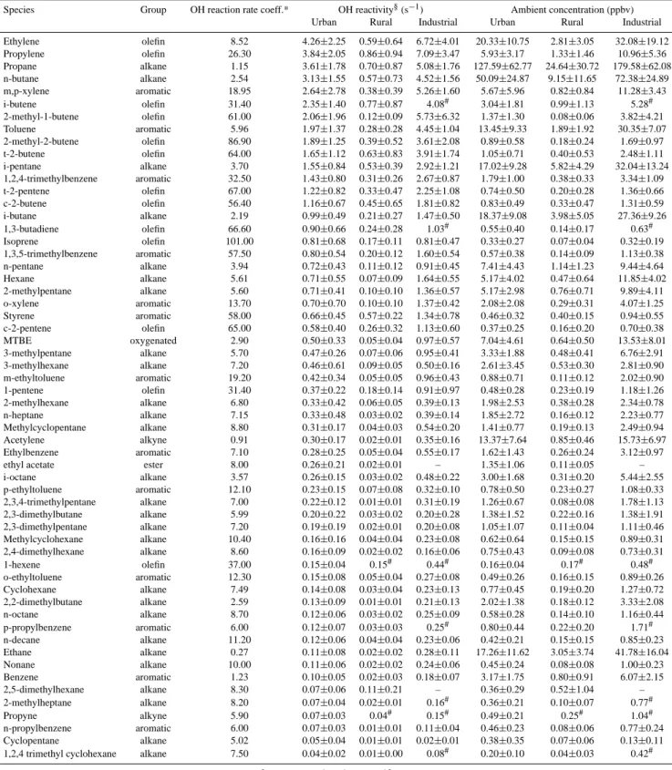
It is useful to examine the VOC distribution in an ur-ban area in terms of reactivity with the hydroxyl radical (OH), which in fact represents the contribution of each VOC species to the OH loss rate. The OH loss rate is a measure of the initial peroxy radical formation rate, which is frequently the rate-limiting step in ozone formation. The actual amount of ozone produced by a given hydrocarbon depends on their particular oxidation mechanism, the abundance of other hy-drocarbons, and NOx concentrations (Carter, 1994). While
realizing that this approach does not account for the full at-mospheric chemistry of the compounds considered, it pro-vides a useful approximation of their relative contributions to daytime photochemistry. For this purpose, Table 4 lists the major hydrocarbons in the atmosphere of the Valley of Mexico by reactivity with OH along with their average
am-Table 4. OH reactivity and average ambient concentrations of major NMHC measured during the MCMA-2002 and 2003 studies at urban (Pedregal, La Merced, CENICA and Constituyentes), rural (Santa Ana Tlacotenco, Teotihuacan and La Reforma) and industrial (Xalostoc) sites of the Valley of Mexico. Data correspond to the morning rush hours (6:00 to 9:00 h). The numbers at the right of the ± symbol indicate one standard deviation.
Species Group OH reaction rate coeff.* OH reactivity§(s−1) Ambient concentration (ppbv) Urban Rural Industrial Urban Rural Industrial Ethylene olefin 8.52 4.26±2.25 0.59±0.64 6.72±4.01 20.33±10.75 2.81±3.05 32.08±19.12 Propylene olefin 26.30 3.84±2.05 0.86±0.94 7.09±3.47 5.93±3.17 1.33±1.46 10.96±5.36 Propane alkane 1.15 3.61±1.78 0.70±0.87 5.08±1.76 127.59±62.77 24.64±30.72 179.58±62.08 n-butane alkane 2.54 3.13±1.55 0.57±0.73 4.52±1.56 50.09±24.87 9.15±11.65 72.38±24.89 m,p-xylene aromatic 18.95 2.64±2.78 0.38±0.39 5.26±1.60 5.67±5.96 0.82±0.84 11.28±3.43 i-butene olefin 31.40 2.35±1.40 0.77±0.87 4.08# 3.04±1.81 0.99±1.13 5.28# 2-methyl-1-butene olefin 61.00 2.06±1.96 0.12±0.09 5.73±6.32 1.37±1.30 0.08±0.06 3.82±4.21 Toluene aromatic 5.96 1.97±1.37 0.28±0.28 4.45±1.04 13.45±9.33 1.89±1.92 30.35±7.07 2-methyl-2-butene olefin 86.90 1.89±1.25 0.39±0.52 3.61±2.08 0.89±0.58 0.18±0.24 1.69±0.97 t-2-butene olefin 64.00 1.65±1.12 0.63±0.83 3.91±1.74 1.05±0.71 0.40±0.53 2.48±1.11 i-pentane alkane 3.70 1.55±0.84 0.53±0.39 2.92±1.21 17.02±9.28 5.82±4.29 32.04±13.24 1,2,4-trimethylbenzene aromatic 32.50 1.43±0.80 0.31±0.26 2.67±0.87 1.79±1.00 0.38±0.33 3.34±1.09 t-2-pentene olefin 67.00 1.22±0.82 0.33±0.47 2.25±1.08 0.74±0.50 0.20±0.28 1.36±0.66 c-2-butene olefin 56.40 1.16±0.67 0.45±0.65 1.81±0.82 0.83±0.49 0.33±0.47 1.31±0.59 i-butane alkane 2.19 0.99±0.49 0.21±0.27 1.47±0.50 18.37±9.08 3.98±5.05 27.36±9.26 1,3-butadiene olefin 66.60 0.90±0.66 0.24±0.28 1.03# 0.55±0.40 0.14±0.17 0.63# Isoprene olefin 101.00 0.81±0.68 0.17±0.11 0.81±0.47 0.33±0.27 0.07±0.04 0.32±0.19 1,3,5-trimethylbenzene aromatic 57.50 0.80±0.54 0.20±0.12 1.60±0.54 0.57±0.38 0.14±0.09 1.13±0.38 n-pentane alkane 3.94 0.72±0.43 0.11±0.12 0.91±0.45 7.41±4.43 1.14±1.23 9.44±4.64 Hexane alkane 5.61 0.71±0.55 0.07±0.09 1.64±0.55 5.17±4.02 0.47±0.64 11.85±4.02 2-methylpentane alkane 5.60 0.71±0.41 0.10±0.10 1.36±0.57 5.17±2.98 0.76±0.71 9.89±4.11 o-xylene aromatic 13.70 0.70±0.70 0.10±0.10 1.37±0.42 2.08±2.08 0.29±0.31 4.07±1.25 Styrene aromatic 58.00 0.66±0.45 0.57±0.22 1.34±0.78 0.46±0.32 0.40±0.15 0.94±0.55 c-2-pentene olefin 65.00 0.58±0.40 0.26±0.32 1.13±0.60 0.37±0.25 0.16±0.20 0.70±0.38 MTBE oxygenated 2.90 0.50±0.33 0.05±0.04 0.97±0.57 7.04±4.61 0.64±0.50 13.53±8.01 3-methylpentane alkane 5.70 0.47±0.26 0.07±0.06 0.95±0.41 3.33±1.88 0.48±0.41 6.76±2.91 3-methylhexane alkane 7.20 0.46±0.61 0.09±0.05 0.50±0.16 2.61±3.45 0.53±0.30 2.81±0.90 m-ethyltoluene aromatic 19.20 0.42±0.34 0.05±0.05 0.96±0.43 0.88±0.71 0.11±0.12 2.02±0.90 1-pentene olefin 31.40 0.37±0.22 0.18±0.14 0.91±0.97 0.48±0.28 0.23±0.19 1.18±1.26 2-methylhexane alkane 6.80 0.33±0.42 0.06±0.05 0.39±0.13 1.98±2.53 0.38±0.28 2.34±0.78 n-heptane alkane 7.15 0.33±0.48 0.03±0.02 0.39±0.14 1.85±2.72 0.16±0.12 2.23±0.77 Methylcyclopentane alkane 8.80 0.31±0.17 0.04±0.03 0.54±0.20 1.41±0.77 0.19±0.13 2.49±0.94 Acetylene alkyne 0.91 0.30±0.17 0.02±0.01 0.35±0.16 13.37±7.64 0.85±0.46 15.73±6.97 Ethylbenzene aromatic 7.10 0.28±0.25 0.05±0.04 0.55±0.17 1.62±1.43 0.26±0.24 3.12±0.97 ethyl acetate ester 8.00 0.26±0.21 0.02±0.01 – 1.35±1.06 0.11±0.05 – i-octane alkane 3.57 0.26±0.15 0.03±0.02 0.48±0.22 3.00±1.68 0.31±0.20 5.44±2.55 p-ethyltoluene aromatic 12.10 0.23±0.15 0.07±0.08 0.32±0.10 0.78±0.50 0.23±0.27 1.08±0.33 2,3,4-trimethylpentane alkane 7.00 0.22±0.12 0.01±0.01 0.31±0.19 1.26±0.67 0.08±0.08 1.78±1.13 2,3-dimethylbutane alkane 5.99 0.20±0.22 0.03±0.02 0.20±0.28 1.38±1.52 0.22±0.16 1.38±1.91 2,3-dimethylpentane alkane 7.20 0.19±0.19 0.02±0.01 0.20±0.08 1.05±1.07 0.11±0.04 1.11±0.46 Methylcyclohexane alkane 10.40 0.16±0.16 0.04±0.04 0.23±0.08 0.62±0.64 0.15±0.15 0.89±0.31 2,4-dimethylhexane alkane 8.60 0.16±0.09 0.02±0.02 0.16±0.06 0.75±0.43 0.09±0.08 0.73±0.31 1-hexene olefin 37.00 0.15±0.04 0.15# 0.44# 0.16±0.04 0.17# 0.48# o-ethyltoluene aromatic 12.30 0.15±0.08 0.05±0.04 0.27±0.08 0.49±0.26 0.16±0.15 0.89±0.26 Cyclohexane alkane 7.49 0.14±0.08 0.03±0.04 0.23±0.13 0.77±0.45 0.19±0.20 1.27±0.72 2,2-dimethylbutane alkane 2.59 0.13±0.09 0.01±0.01 0.21±0.13 2.02±1.38 0.18±0.12 3.33±2.08 n-octane alkane 8.70 0.12±0.06 0.03±0.02 0.25±0.09 0.58±0.28 0.14±0.10 1.16±0.44 p-propylbenzene aromatic 6.00 0.12±0.07 0.03±0.03 0.25# 0.80±0.44 0.22±0.20 1.71# n-decane alkane 11.20 0.12±0.06 0.04±0.04 0.23±0.06 0.42±0.21 0.15±0.15 0.85±0.23 Ethane alkane 0.27 0.11±0.08 0.02±0.02 0.28±0.11 17.26±11.62 3.05±3.74 41.78±16.04 Nonane alkane 10.00 0.11±0.06 0.02±0.02 0.24±0.06 0.45±0.24 0.08±0.08 1.00±0.23 Benzene aromatic 1.23 0.10±0.05 0.02±0.03 0.18±0.07 3.17±1.75 0.80±0.91 6.07±2.15 2,5-dimethylhexane alkane 8.30 0.07±0.06 0.11±0.21 – 0.36±0.29 0.52±1.04 – 2-methylheptane alkane 8.20 0.07±0.04 0.02±0.01 0.16# 0.36±0.21 0.10±0.07 0.77# Propyne alkyne 5.90 0.07±0.03 0.04# 0.15# 0.49±0.21 0.25# 1.04# n-propylbenzene aromatic 6.00 0.07±0.03 0.01±0.01 0.11±0.04 0.46±0.23 0.08±0.06 0.77±0.24 Cyclopentane alkane 5.02 0.05±0.04 0.01±0.01 0.02±0.01 0.38±0.35 0.07±0.06 0.13±0.11 1,2,4 trimethyl cyclohexane alkane 7.50 0.04±0.02 0.01±0.00 0.08# 0.20±0.10 0.04±0.03 0.42#
* OH reaction rate coefficients at 298 K and 1 atm (cm3molecule−1s−1)×10−12, (Atkinson, 1994, 1997).
§Products of mean individual VOC concentrations and OH reaction rate coefficients. To obtain the OH reactivity in units of s−1the VOC
ambient concentrations were transformed to units of molecule cm−3.
bient concentrations during the morning rush hour. Average reactivity levels and concentrations are shown in columns ac-cording to the site type: urban, rural (Santa Ana Tlacontenco, La Reforma and Teotihuacan) and industrial (Xalostoc). For the urban sites, the reactivity values were calculated indepen-dently for each monitored site but, as the results were quite similar, only the reactivity values calculated for the average concentrations are presented. VOCs are sorted in descend-ing order accorddescend-ing to their reactivity in urban sites. It is important to point out that many oxygenated VOCs and car-bonyls were not considered in this analysis, and therefore it is more appropriate to use the term non methane hydrocarbons (NMHC) instead of VOCs. The OH reaction rate coefficients shown in Table 4 correspond to the coefficients published by Atkinson (1994, 1997) at 298 K and 1 atm. Where no infor-mation was available, the OH reaction rate coefficient was estimated from information on similar compounds.
The ten most important NMHC in the urban atmosphere of the Valley of Mexico in terms of OH reactivity include two aromatics, six olefins and two alkanes: ethylene, propy-lene, propane, n-butane, m,p-xylenes, i-butene, 2-methyl-1-butene, toluene, 2-methyl-2-butene and t-2-butene. It is im-portant to point out that the two most reactive NMHC at urban sites were also the top two NMHC reported for the industrial site. These species are olefins mainly emitted by vehicles with high concentrations and high reaction rate co-efficients. Also, it is important to highlight that the elevated concentrations of propane and n-butane are sufficient to rank these two alkanes among the top 5 NMHC, even though their reactivity rate coefficients are small compared to those for olefins and aromatics. Using a Total OH Loss Measurement instrument (TOHLM) Shirley et al. (2006) measured an OH reactivity of ∼120 s−1during the morning rush hours at the
CENICA site and estimated that 72% of it was due to VOCs. Overall, major NMHC in terms of ozone production in the Valley of Mexico are of anthropogenic origin. Biogenic NMHC seem to be relatively insignificant. Isoprene concen-trations were low (0.33±0.27 ppbv in urban sites) compared to other reactive species, and were assumed to have their ori-gin more from vehicle exhaust than from vegetation. Differ-ent studies have reveled that the isoprene has a strong anthro-pogenic origin (Borbon et al., 2001), particularly in urban ar-eas with scarce vegetation. The olefin fluxes mar-easured at the urban site of CENICA did not show the typical biogenic peak of isoprene around noon when solar radiation and tempera-ture are highest (Velasco et al., 2005). With the knowledge that 1,3-butadiene is a good tracer for vehicle exhaust (Ye et al., 1997), we compared the morning ambient concentra-tions of isoprene and 1,3-butadiene measured at the urban sites. The regression between these two species was nearly linear; although it showed some dispersion, it suggests that both species share the same emission sources. Using the on-road samples collected by the Aerodyne mobile-laboratory, which are described in detail in Sect. 5.4, we found an iso-prene to 1,3-butadiene ratio of 0.27, comparable to the
ra-tio of 0.30 obtained for the ambient samples at the urban sites. These ratios are similar to those reported for other ur-ban and suburur-ban sites (Borbon et al., 2001; Reinmann et al., 2000). Vegetation was sparse at the three monitored ru-ral sites, and, therefore, isoprene concentrations were also low (0.07±0.04 ppbv). At rural sites, low molecular weight alkanes were the most abundant species, emitted from LPG leakages as it has been discussed before. At rural sites, one of the most reactive hydrocarbons was styrene, with ambi-ent concambi-entrations similar to those observed at urban sites (0.57±0.22 ppbv). The presence of styrene in these rural en-vironments is attributed to local biomass and trash burning.
A comparison of the reactivity levels between the urban sites and industrial site indicates that on average the air in the industrial location is 1.8 times more reactive than at the urban sites. Half of the measured VOCs at the industrial site had reactivity levels between 1.4 and 2.1 times higher than at the urban sites. A similar comparison between urban and rural sites shows that the urban atmosphere is 4.6 times more reactive than the rural atmosphere in the Valley of Mexico. 5.3 Distribution of VOCs by compound type
Figure 6 shows the VOC distributions by compound type during the morning (6:00 to 9:00 h) and afternoon (12:00 to 15:00 h) from canister samples collected and analyzed by the WSU and IMP groups. Note that concentrations are in ppbC. Hereafter all contribution fractions are based on ppbC, as well. In the morning, the entire valley experi-ences a relatively homogeneous mix of VOCs consisting of ∼60% alkanes, ∼15% aromatics, ∼5% olefins and a remain-ing 20% of alkynes, halogenated hydrocarbons, oxygenated species (esters, ethers, carbonyls, etc.) and other unidenti-fied VOCs. In our study, concentrations of total VOCs in the industrial area were 1.6 times higher than at urban sites dur-ing the morndur-ing period, while concentrations at rural sites were about one-sixth of those measured at the urban loca-tions. In the afternoon, VOC concentrations were less and the distribution among species was different with a higher contribution of unidentified VOCs at the urban sites. The re-duction in concentrations from morning to afternoon were: alkanes 70%, olefins 60%, aromatics 53%, and unidentified VOCs 20%. Lower afternoon concentrations are normally ascribed to increased dispersion and photochemical oxida-tion during the midday period. However, employing these mechanisms alone is insufficient to explain those reductions, because the relatively unreactive alkanes showed the largest proportional loss. Emission rates must be a factor, as well, with a large decrease in alkane emissions relative to aromat-ics and olefins. A reduction in the emission rate of alkanes from morning to afternoon could be due to reduced consump-tion of LPG (propane, i-butane, n-butane) during the after-noon hours. LPG is used by Mexican household to heat wa-ter for bathing and showering prior to going to work in the morning. Leakage from LPG transmission systems will be
largest during the morning period of maximum usage. Santa Ana Tlacotenco, a rural downwind boundary site, showed an opposite pattern. Relatively low local emissions coupled with transport emissions from the urban region resulted in af-ternoon VOC concentrations 2.4 higher than in the morning.
Hydrocarbons. At urban and industrial sites during the
morning period, hydrocarbons with four or less carbons rep-resent the major fraction of the alkanes and alkenes. The main contributors are propane, n-butane, ethylene, propy-lene, and the sum of i-, t-2- and -c-2 butenes. 1,3-butadiene is a four-carbon diene that is considered to be a carcinogenic and reproductive toxicant to humans, whose main source is vehicle exhaust (USEPA, 1999b). 1,3-butadiene is of cern in Mexico City because of its relatively elevated con-centrations: 0.55 and 0.63 ppbv at urban and industrial sites, respectively.
The most abundant aromatics were the BTEX species (benzene, toluene ethylbenzene and the xylene isomers). They accounted for about 75% of the aromatic burden. The average toluene concentration was 13.45±9.33 ppbv at ur-ban sites and 30.35±7.07 ppbv at the industrial area. To-tal xylene concentrations averaged 15.35±4.68 ppbv at the industrial site and about half of that (7.75±8.14) in the ur-ban area. Ethylbenzene had average concentrations about the same as the individual xylene isomers with concen-trations of 1.62±1.43 ppbv in the urban areas and about 3.12±0.97 ppbv in the industrial region. Benzene averaged 6.07±2.15 and 3.17±1.75 ppbv at the industrial and urban sites, respectively. The urban benzene concentration deter-mined in this study is similar to that reported by Bravo et al. (2002) for residential areas in southwest Mexico City.
Oxygenated hydrocarbons. MTBE is the only oxy-genated VOC listed in Table 4. MTBE is used as an ad-ditive in unleaded gasoline to enhance the combustion effi-ciency. In our canister samples, MTBE contributes no more than 2% to the total VOC burden of the Valley of Mexico. Ethyl tertiary butyl ether (ETBE) was another oxygenated VOC identified in the samples analyzed by IMP. ETBE is not included in Table 4 because it was measured at only half of the sites (Xalostoc, Pedregal, CENICA and La Merced). Av-erage ETBE concentrations were 0.3 and 0.6 ppbv at urban and industrial sites, respectively, 96% lower than the aver-age MTBE concentrations at both types of site. Both MTBE and ETBE have their origin from vehicle exhaust due to in-complete combustion and gasoline evaporation from fueling stations and vehicle gasoline tanks.
During the MCMA-2003 study, ambient concentrations of formaldehyde were measured by DOAS at two different sites: CENICA and La Merced. The monthly average con-centrations at CENICA and La Merced were 8.2±4.6 and 6.0±4.7 ppbv, respectively (Volkamer et al., 2005; Grutter et al., 2005). Garcia et al. (2005) determined on a 24 h average basis, that mobile and industrial sources contribute 42% to the ambient concentration of formaldehyde, the atmospheric oxidation of numerous VOCs contribute greater than 38%
Fig. 6. VOC distribution by compound type during the morning (a) and afternoon (b). Numbers in the columns indicate the percent contribution of each VOC group to the total VOC concentration, which is displayed at the bottom of each column in ppbC.
and the remaining 20% is due mainly to uncounted industrial processes.
Glyoxal was another oxygenated hydrocarbon detected di-rectly by DOAS at the CENICA site in 2003. Volkamer et al. (2005) found that glyoxal is predominantly formed from
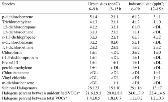
Table 5. Ambient average concentrations of halogenated VOCs measured during the MCMA-2003 study at urban (Pedregal, La Merced and CENICA) and industrial (Xalostoc) sites of the Valley of Mexico. The numbers at the right of the ± symbol indicate one standard deviation. Concentrations below the detection limit are indicate as <DL.
Species Urban sites (ppbC) Industrial site (ppbC) 6–9 h 12–15 h 6–9 h 12–15 h p-dichlorobenzene 5±4 2±1 6±2 3±1 Trichloroethylene 4±3 2±1 4±2 1±0 1,2-dichloropropane 4±2 3±1 0±0 <DL 1,2-dichloroethane 3±3 2±2 1±1 <DL c-1,3-dichlopropene 3±3 2±1 6±3 4±2 o-dichlorobenzene 3±2 0±0 5±1 <DL 1,1-dichloroethane 2±2 2±2 1±2 2±2 Chloroform 1±1 <DL 3±2 1±0 t-1,3-dichloropropene 1±1 <DL 1±1 <DL Freon113 1±1 1±1 1±1 <DL perchloroethylene 1±1 <DL 1±1 <DL Chlorobenznene <DL <DL <DL 1±1 Vinyl chloride <DL <DL <DL 1±1 m-dichlorobenzene <DL 1±1 <DL <DL Subtotal Halogenates 28±23 15±10 29±16 13±7
Halogens percent between unidentified VOCs* 21.6±9.1 20.0±8.8 24.0±3.9 22.4±4.6 Halogens percent between total VOCs* 1.4±0.5 1.8±0.7 1.1±0.2 1.2±0.3 * These average percents were calculated with the samples in which halogenated VOCs were analyzed.
airborne VOC oxidation in the atmosphere of Mexico City, reaching peaks around 1.8 ppbv between 10 and 13:00 h. The ambient concentrations of glyoxal were about one order of magnitude less affected by vehicle emissions than those of formaldehyde, and thus present a well suitable indicator molecule for VOC oxidation processes.
Halogenated hydrocarbons. The GC-FID technique can
be used to identify halogenated VOCs, but not to precisely quantify their concentration, since halogenated VOCs con-tain other atoms besides carbon and hydrogen. However, IMP quantified 14 halogenated VOCs at the Xalostoc, Pe-dregal, CENICA and La Merced sites. Table 5 shows that the set of identified halogenated species contributes less than 2% to the total VOC burden. All of them are emitted by an-thropogenic sources. Many of them are classified as toxic and carcinogenic species, and others, such as the vinyl chlo-ride, are suspected to cause congenital malformation (IPCS, 2005). Another concern is the very long atmospheric resi-dence times of some halogenated VOCs, in particular chlo-rofluorocarbons such as Freon 113. They can eventually dif-fuse into the stratosphere where photolysis produces chlorine radicals, which catalytically destroy ozone and indirectly contribute to the greenhouse effect. Even though the use of chlorofluorocarbons as refrigerants is not allowed anymore, chlorofluorocarbon emissions occur during the disposal of old refrigeration units and, in developing cities such as Mex-ico City, leakage from old residential refrigerators may also be a significant source.
5.4 Comparison of ambient VOC concentrations to vehi-cles exhaust signatures
Since roadway vehicle emissions are normally the dominant VOC source in urban areas (Watson et al., 2001), it was of interest to compare the mixing ratios obtained from canister sampling at the urban sites to the vehicle exhaust source sig-nature measured during mobile vehicle chase experiments.
Briefly, vehicle chase measurements were made using the Aerodyne mobile laboratory equipped with several instru-ments to characterize emissions from vehicles under actual driving conditions (see Herndon et al., 2005; Herndon et al., 20072; Zavala et al., 2006; Rogers et al., 2007). In chase mode, the Aerodyne van was driven immediately be-hind a selected vehicle for approximately 5 to 20 min. Ve-hicle plume samples were collected with an auto-sampling system that included a fast response CO2sensor (LICOR
LI-7000). Distinct peaks in the CO2mixing ratio during a
vehi-cle chase indicated interception of the exhaust plume. When the CO2 levels were elevated above a selected threshold, a
conditional VOC sampler was manually activated to sample into a “chase” canister and when CO2levels were below the
threshold, air was channeled into an “on-road background” canister (Herndon et al., 2005, 20072).
2Herndon, S. C., Kolb, C. E., Lamb, B., Westberg, H., Allwine,
E., Velasco, E., Knighton, B., Zavala, M., Molina, L. T. and Molina, J. M.: Conditional sampling of volatile organic compounds in on-road vehicle plumes, in preparation, 2007.)
Table 6. Hydrocarbon molar ratios (ppbC/ppbC) measured at the industrial, urban and rural sites and from vehicle chase operation during the MCMA-2002 and 2003 field studies. Also ratios from vehicles exhaust studies in North America are shown for comparison.
Industrial Urban Rural Vehicular chases Mexican gasoline Mexican diesel US & Canada light vehicles§ vehicles§ duty vehicles#
G. Mean* Median G. mean* Median G. mean* Median G. mean* Median Average Average Average@
Alkene ratios t-2-butene/c-2-butene 1.53±0.91 1.25 1.28±0.83 1.21 1.52±0.66 1.48 1.11±0.50 1.10 1.17 1.00 1.27±0.33 t-2-pentene/c-2-pentene 1.71±0.51 1.91 1.97±0.53 2.07 1.75±0.51 1.89 1.93±0.46 1.98 – 9.33 1.78±0.19 1-hexene/1-pentene 0.46±0.46 0.52 0.52±0.48 0.59 – – – – – – 0.49±0.25 1,3-butadiene/t-2-pentene 0.98±0.58 1.14 0.78±0.52 0.77 0.56±0.47 0.64 0.87±0.97 0.96 – – 1.36±0.51 propylene/ethylene 0.45±0.30 0.44 0.50±0.68 0.42 0.38±0.28 0.44 0.51±0.37 0.50 0.55 0.71 0.30±0.04 Alkane ratios i-butane/n-butane 0.38±0.04 0.37 0.37±0.03 0.37 0.40±0.07 0.41 0.36±0.04 0.36 0.32 0.48 0.19±0.08 i-pentane/n-pentane 3.58±0.69 3.62 2.80±1.41 2.59 6.96±6.61 8.08 2.57±1.69 2.36 2.63 4.27 2.97±0.57 2-methylpentane/ 1.36±0.19 1.41 1.51±1.80 1.54 1.57±0.78 1.59 1.48±0.14 1.47 1.67 1.18 1.69±0.11 3-methylpentane Hexane/2-methylpentane 1.11±0.31 1.11 0.71±0.40 0.72 0.67±0.83 0.69 0.62±0.15 0.65 0.78 1.02 0.52±0.05 Cyclohexane/n-heptane 0.78±1.03 0.50 0.56±0.60 0.50 0.76±0.74 0.91 0.61±0.63 0.54 0.86 0.29 0.43±0.17 n-octane/nonane 0.76±0.38 1.01 1.39±0.82 1.29 1.14±0.62 1.12 1.30±0.43 1.28 1.04 0.55 1.49±0.05 Aromatic ratios Toluene/benzene 8.10±4.57 8.81 5.06±2.32 4.89 3.53±1.35 3.45 3.96±1.34 3.80 2.78 5.05 1.59±0.28 ethylbenzene/toluene 0.08±0.04 0.09 0.12±0.05 0.13 0.15±0.07 0.15 0.14±0.05 0.15 0.21 0.30 0.17±0.03 isopropylbenzene/toluene 0.010±0.005 0.01 0.010±0.008 0.020 – – – – 0.027 0.016 0.020±0.008 o-xylene/m,p-xylene 0.36±0.03 0.36 0.40±0.07 0.39 0.38±0.11 0.40 0.39±0.05 0.39 0.39 0.36 0.38±0.02 Styrene/ 0.88±0.68 0.98 1.16±1.67 1.22 3.45±3.58 3.10 0.57±0.42 0.55 0.37 0.84 0.81±0.21 1,3,5-trimethylbenzene 1,2,3-trimethylbenzene/ 0.38±0.09 0.36 0.40±0.13 0.37 – – – – – – 0.25±0.07 1,2,4-trimethylbenzene
* Geometric mean ± 1 standard deviation.
§From vehicle emission profiles measured in Mexico City in 1998 (Mugica et al., 2001b).
#Average vehicle exhaust ratio calculated by Jobson et al. (2004) from six tunnel studies conducted in the 1990s (Conner et al., 1995;
Kirchstetter et al., 1996; Sagebiel et al., 1996; Fraser et al., 1998; Rogak et al., 1998).
@Average ± 1 standard deviation.
For the comparison between ambient and vehicular emis-sion data, it is necessary to remove the impact of photo-chemical aging on source signatures. This is achieved by regressions between species with similar atmospheric life-times. The source ratio is preserved for species with simi-lar lifetimes because photochemical loss and mixing will re-sult in similar rates of concentration change (Parrish et al., 1998). This procedure allowed all of the ambient data to be used, including afternoon data when mixing ratios were typ-ically lower due to mixing and photochemical removal. The slope obtained in ambient data plots defines the source ratio that can be directly compared to the vehicular chase mea-surements and literature values. In practice, there are a lim-ited number of species that can be employed in this analysis because photochemical loss rates must be similar. We have generally constrained the hydrocarbon pairings such that OH rate coefficients differ by 20% or less. The exception is the regression between propylene and ethylene where rate con-stants differ by a factor of three.
Correlations between selected alkenes, alkanes and aro-matics are shown in Figs. 7, 8 and 9, respectively. The ge-ometric mean ratios from the vehicular chase data and from the ambient sampling at urban, rural and industrial sites are
tabulated in Table 6. In addition, Table 6 shows average ex-haust ratios for Mexican gasoline and diesel vehicles from a tunnel study conducted in Mexico City (Mugica et al., 2001b). An average vehicle exhaust ratio for light duty ve-hicles calculated by Jobson et al. (2004) from six published tunnel studies conducted in the 1990s in US and Canada is included in the table, as well.
In the alkene group, t-2-pentene versus c-2-pentene ex-hibits excellent agreement between the ambient and vehic-ular emission ratios. The ambient concentrations span three orders of magnitude due to atmospheric processing and vari-ations in source strength. In general, the highest concentra-tions were recorded during vehicular chase experiments. In a few cases, ambient industrial and urban samples approached vehicle chase concentrations. The very good agreement be-tween the exhaust emission and ambient ratios for the 2-pentenes clearly implies a vehicle exhaust source signature. The t-2-butene versus the c-2-butene correlation shows rea-sonable agreement between vehicular chase emissions, bient ratios and literature values. The similarity of the am-bient and vehicle exhaust ratios for these species suggests vehicle exhaust as their primary source. For hexene and 1-pentene, ambient data showed considerable scatter
suggest-Fig. 7. Correlations between alkenes comparing ambient data to vehicle chase samples. Ambient data correspond to all canister samples and the dashed line indicates the regression line for vehicular chase data.
ing that each site is impacted by a mix of different sources, and that sources and emission rates of 1-hexene are not strongly correlated with sources and emission rates of 1-pentene. The propylene:ethylene ratio displays a fair cor-relation but contains considerable scatter. The vehicle emis-sion ratio (0.51±0.37) bisects the ambient data, but the large amount of scatter about this ratio is indicative of multiple in-dependent sources. The exhaust emissions ratio itself has a high degree of scatter, suggesting that the emission relation of these species may vary considerably within the Mexican
fleet. As indicated previously, propylene and ethylene rate constants vary much more than for the other alkene pairs, which may contribute also to the poor correlations observed for these species.
Ratios for i-butane:n-butane showed excellent agreement between the ambient, vehicular emission and literature val-ues. Note that the average ratios in Table 6 for ambient (0.38 industrial and 0.37 urban) and vehicle exhaust (0.36) are es-sentially equal. Mugica et al. (2001b) reported exhaust emis-sion ratios of 0.32 and 0.48 for gasoline and diesel vehicles in
Fig. 8. Correlations between alkanes comparing ambient data to vehicle chase samples. Ambient data correspond to all canister samples and the dashed line indicates the regression line for vehicular chase data.
Mexico. These results suggest that vehicle exhaust is also an important source of n-butane and i-butane in addition to LPG leakage. Mugica et al. (2002b) through a source apportion-ment analysis determined that vehicle exhaust contributes 20% to the emission of these two alkanes, while handling and
distribution of LPG releases ∼65%. Although LPG powered vehicles represent less than 1% of the total fleet, they should also be considered important sources. Schifter et al. (2000) evaluated the LPG vehicles program implemented in Mexico City and found that 95% of them have emissions that exceed
Fig. 9. Correlations between aromatics comparing ambient data to vehicle chase samples. Ambient data correspond to all canister samples and the dashed line indicates the regression line for vehicular chase data.
those required by environmental regulations. The LPG fleet is composed mainly of vehicles used intensively (light and heavy duty trucks, and small buses with 20-passenger capac-ity). Gasca et al. (2004) reported that tailpipe and evaporative emissions of i-butane contribute 16% and 28%, respectively,
to the total VOC emissions from LPG vehicles, and 17% and 21% of n-butane.
Good agreement between 2-methylpentane: 3-methylpentane ambient, vehicle chase and literature ratios implicate vehicle exhaust emissions as the primary