Multi-Decadal Trends of Global Surface Temperature: A Broken Line with Alternating ~30 yr Linear Segments?

(1)

HAL Id: insu-00944085

https://hal-insu.archives-ouvertes.fr/insu-00944085

Submitted on 7 Aug 2020

HAL is a multi-disciplinary open access archive for the deposit and dissemination of sci-entific research documents, whether they are pub-lished or not. The documents may come from teaching and research institutions in France or abroad, or from public or private research centers.

L’archive ouverte pluridisciplinaire HAL, est destinée au dépôt et à la diffusion de documents scientifiques de niveau recherche, publiés ou non, émanant des établissements d’enseignement et de recherche français ou étrangers, des laboratoires publics ou privés.

Multi-Decadal Trends of Global Surface Temperature: A

Broken Line with Alternating 30 yr Linear Segments?

Vincent Courtillot, Jean-Louis Le Mouel, Vladimir Kossobokov, Dominique

Gibert, Fernando Lopes

To cite this version:

Vincent Courtillot, Jean-Louis Le Mouel, Vladimir Kossobokov, Dominique Gibert, Fernando Lopes. Multi-Decadal Trends of Global Surface Temperature: A Broken Line with Alternating 30 yr Linear Segments?. Atmospheric and Climate Sciences, Scientific Research Publishing, 2013, 3, pp.364-371. �10.4236/acs.2013.33038�. �insu-00944085�

(2)

Multi-Decadal Trends of Global Surface Temperature: A

Broken Line with Alternating ~30 yr Linear Segments?

Vincent Courtillot1_{, Jean-Louis Le Mouël}1_{, Vladimir Kossobokov}1,2_,

Dominique Gibert1_{, Fernando Lopes}1

1_{Geomagnetism and Paleomagnetism, Institut de Physique du Globe de Paris, Université Paris Diderot,}

Sorbonne Paris Cité, 1 rue Jussieu, Paris, France

2_{Institute of Earthquake Prediction Theory and Mathematical Geophysics, Russian Academy of Sciences,}

Moscow, Russia Email: courtil@ipgp.fr

Received March 12, 2013; revised April 15, 2013; accepted April 23, 2013

Copyright © 2013 Vincent Courtillot et al. This is an open access article distributed under the Creative Commons Attribution Li- cense, which permits unrestricted use, distribution, and reproduction in any medium, provided the original work is properly cited.

ABSTRACT

We investigate global temperature data produced by the Climate Research Unit at the University of East Anglia (CRU) and the Berkeley Earth Surface Temperature consortium (BEST). We first fit the 1850-2010 data with polynomials of degrees 1 to 9. A significant ~60-yr oscillation is accounted for as soon as degree 4 is reached. This oscillation is even better modeled as a broken line, more precisely a series of ~30-yr long linear segments, with slope breaks (singularities) in ~1904, ~1940, and ~1974 (±3 yr), and a possible recent occurrence at the turn of the 20th century. Oceanic indices PDO (Pacific Decadal Oscillation) and AMO (Atlantic Multidecadal Oscillation) have undergone major changes (respectively of sign and slope) roughly at the same times as the temperature slope breaks. This can be interpreted with a system of oceanic non-linear coupled oscillators with abrupt mode shifts. Thus, the Earth’s climate may have entered a new mode (a new ~30-yr episode) near the turn of the 20th century: no further temperature increase, a dominantly negative PDO index and a decreasing AMO index might be expected for the next decade or two.

Keywords: Global Surface Temperature; Multi-Decadal Evolution; Linear Segments; ~60-Year Oscillation

1. Introduction

Global surface temperatures are one of the parameters most commonly used to discuss the evolution of climate. Databases of instrumental temperatures that cover the past century and a half have been compiled by four main groups (Climate Research Unit at the University of East Anglia—CRU, NASA Goddard Institute for Space Stud- ies—GISS, National Oceanic and Atmospheric Adminis- tration—NOAA, Berkeley Earth Surface Temperature consortium—BEST). This is a huge, difficult task and these databases are necessarily faced with a number of limitations: the geographical distribution of stations is far from uniform and varies with time; also, there may be fundamental difficulties in establishing meaningful global temperatures for the Earth [1]. Climate is generally defined as the ~30 year average of weather and since only 100 to 150 years of instrumental data are available, this places severe limitations on the significance of global temperature trends and multi-decadal oscillations. A monotonic (low degree) trend can be fit to all global tem-

perature data sets over the period from 1850 to the present. This trend amounts to a secular rise of ~1 K over the period. Once this trend is removed, a ~60 yr oscillation stands out in most records. Such an oscillation has been discussed for instance by [2] and [3]. Lean and Rind [4,5] have built a model curve for 1889-2006 monthly mean global temperatures, in which they distinguish con- tributions from oceans (using the El Nino Southern Os- cillation ENSO), volcanic aerosols, solar irradiance and anthropogenic forcing. Both observations and their empirical curve display the secular rise of approximately 1 K. But data are lower than model by some 0.2 K around 1910 and higher by 0.2 K around 1940: this is because of the significant ~60 year oscillation identified by previous authors, which is not accounted for by [4].

In this paper, we first check whether some of the main global temperature data sets can be reasonably fit by smooth polynomials of increasing degree from 1 (linear trend) up to 9, with particular focus on the “~60-yr oscillation”. We next suggest that this oscillation may be fit by a series of ~30-yr long linear segments with rather ab-

(3)

V. COURTILLOT ET AL. 365 rupt changes in trend. We find correlations between the

breaks in the multi-decadal trends in global surface temperature and changes in sign of the Pacific Decadal Os- cillation and slope of the Atlantic Multidecadal Oscil- lation indices. We discuss our results in the frame of the dynamical mechanism for major climate shifts proposed by [6].

2. Polynomial Fits to the “~60-yr

Oscillation” in Global Temperatures

We have used monthly temperature anomaly data from the CRU and BEST databases. We chose to use the “raw data” rather than other data-derived products that have been “homogenized” and have thus undergone rather extensive and not always transparent/reproducible data po- lishing. The CRUTem4 database is found at

http://www.cru.uea.ac.uk/cru/data/temperature/. We have analyzed the most recent variance-adjusted (version 4) CRU data from 1850 through 2010 for the whole globe (CRUTem4vGL). We have also analyzed hemispheric and global series CRUTem4-SH, CRUTem4-NH, CRU- Tem4vSH, HadSST2GL, HadCRU3GL, and CRUTEM- 3vGL (these series are described in

http://www.metoffice.gov.uk/hadobs/crutem4/ and [7], and http://www.cru.uea.ac.uk/cru/data/temperature/crutem4v gl.txt), and the Berkeley Earth Surface Temperature (BE- ST) monthly global averages (found at

http://berkeleyearth.org/dataset/, description in [8]). All yield similar results and mainly results based on CRU- Tem4vGL are shown in this paper.

We note in passing differences between the long-term linear or low-degree trends obtained in the various temperature anomaly databases (notwithstanding a possible overall difference in baseline due to the definition of the period with respect to which the anomalies are calculated); the CRU and GISS curves are about 0.3 K below the NOAA and BEST curves in the 2000-2010 decade, whereas all agree to better than 0.1 K between 1920 and 1970 [8]. We return to this in Section 5.

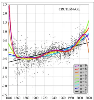
In order to check the significance of the “60-yr oscillation”, we have very simply fit the data sets of monthly mean temperature anomalies (using least squares) with polynomials of increasing degree (Figure 1). The linear (n = 1) trend fit to the CRUTem4vGL data shows the secular rise of approximately 1 K. For n = 2 and 3 the curves fail to account for the “60-yr oscillation” (Figure

1, purple and blue curves). As soon as the degree of the

polynomial reaches 4, the fit accommodates the “60-yr oscillation”, after which the situation remains stable (shown up to n = 9 in Figure 1). Extrapolations of these trends outside of the data domain show quick divergence and are of course meaningless. A ~60 year oscillation would occur only 2.5 times over a 150 yr interval and could not be accounted for by a polynomial of degree

Figure 1. Monthly global temperature anomaly averages from 1850 to 2010 together with least squares polynomial fits with degree from 1 to 9 shown by the color code at lower right. Whole Earth, variance adjusted, CRUTem4vGL database

(http://www.cru.uea.ac.uk/cru/data/temperature/crutem4vg l.txt).

less than ~4.

In order to quantify the goodness of fit, we have calculated the adjusted R-squared values not only for polynomial fits to the data with degrees 1 up to 9 but also for an exponential fit. The adjusted R-squared [9] is a statis- tically unbiased version (i.e. corrected for the number of degrees of freedom) of the R2_{“coefficient of determi-}

nation”, whose main purpose is the prediction of future outcomes on the basis of prior information. R2_{itself is 1}

minus the ratio of variance of errors to variance of observations. The adjusted R-squared values take into consid- eration the number of free parameters of the model (the adjusted R-squared values may be negative when the parameters of the model do not improve the fit compared to the simple average value of the data, which happened in the case of one data set, CRUTem4vSH, that could not be adequately fit by an exponential). In the case of CRU- Tem4vGL, the adjusted R-squared increases significantly from 0.36 (n = 1) to 0.50 (n = 4) and remains stable thereafter (0.52 for n = 9). As soon as the degree exceeds 1 or 2, the adjusted R-squared values for polynomials of degree larger than 3 are larger than for any exponential fit.

3. Broken Line Fits to the “~60-yr

Oscillation” in Global Temperatures

The possibility of fitting ~30-yr long linear segments as an alternative to polynomials or a 60-yr sinusoid to the

(4)

“~60-yr fluctuation” is the topic of this section. Figure

2(a) shows another display of the CRUTem4vGL monthly

data set, limited to the period from 1900 to 2010 (the previous 50 years have significantly larger variance, which is likely due to insufficient, changing station distribution and also possibly to lesser data quality). We note that a series of continuous linear segments with abrupt changes in slope may provide a good fit: such fits have appeared in the literature (e.g. Figure 8 of [10], where linear re- gression lines are shown for intervals 1901-1934, 1934- 1979 and 1979-2010). The most recent has been proposed and discussed by [11], using methods from the dynamics of synchronized chaotic systems.

The models we are seeking belong to the class of “change-point models” [12]. Vasko and Toivonen [13] for instance have published quantitative algorithms to es- timate the number of linear segments to be fit to a time series using permutation tests. We have constructed an algorithm that produces such models, paying particular attention to the management of secondary minima using non-linear simulated annealing. Simulated annealing uses the Metropolis algorithm (see [14-16], for description of the algorithms and definition of terms; see similar use of simulated annealing in [17]). The method is outlined briefly in the Appendix.

We have first tested our method on synthetic data con- sisting of N = 2 to 10 linear segments with variable dura- tions and slopes and varying noise levels from 5% to 25% of the total amplitude range of the data. For each value of N, and for each step of the control parameter, we ran 100 attempts at locating the nodes and displayed the histograms of node locations. For 4 segments and 5% noise, the 3 nodes are identified to within a year in a 2000-month (166 yr) long test series; for 15% noise, de- tection of the 3 nodes is unambiguous but the histograms widen to ~100 months (±4 years uncertainties). For 25% noise, the nodes are still detected but less prominently and with larger uncertainties (~±8 years).

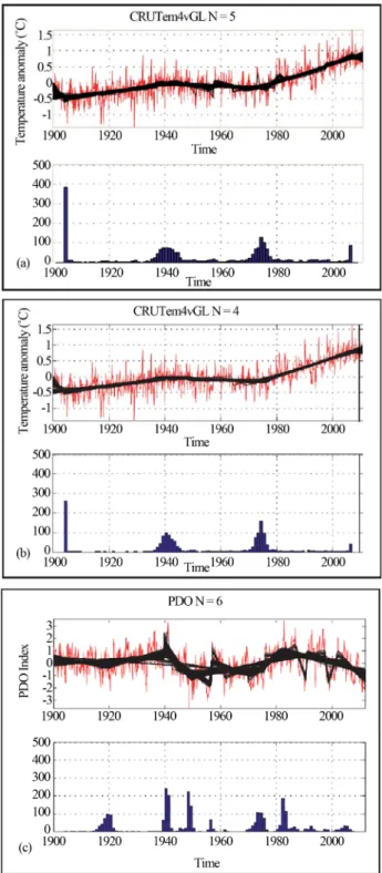
We have then applied the method to the 1900-2010 CRUTem4vGL monthly data, using from 3 to 10 seg- ments. Results are shown in Figure 2(a) for the best case,

i.e. with 5 segments, and in Figure 2(b) with 4 segments

for comparison. Two nodes are clearly identified at ~1940 and ~1974. Two other nodes at ~1904 and ~2006 are near the edges of the data distribution and could be artefacts (end-effects), though this has not been observed with the tests on synthetic data. The ~1904 node appears to be supported by visual inspection of some data pre- dating 1900 (but data dispersion is significantly larger before 1900 than afterwards; see Section 5). The more recent one may require at least a decade of additional data to ascertain its validity. In the case of 4 segments (Figure 2(b)), the histogram does confirm the same 4 nodes with the same dates, although of course each indi-

Figure 2. (a) CRUTem4vGL monthly global temperature anomaly averages from 1900 to 2010 (red curve) and 500 fits of curves made of 5 linear segments (4 nodes) deter- mined with the simulated annealing method described in the text. Below, histogram of node distribution; (b) Same with 4 segments and 3 nodes; (c) Same for the Pacific De- cadal Oscillation Index (PDO) with 6 segments and 5 nodes.

vidual fit out of the 500 realizations must miss one of the 4 clusters seen in the histogram, since only 3 nodes are allowed. The histogram with 6 segments (not shown) still

(5)

V. COURTILLOT ET AL. 367 underlines the same nodes, but with more spread in dates.

As the number of segments is increased to 10, node dis- tributions become more uniform, as segments are used to adjust to shorter (sub-decadal) fluctuations in the data.

The differences in location of the nodes introduce some curvature in the “cloud” of 500 fitted broken lines, but the linear segments between the nodes are quite clear (Figures 2(a) and (b)). We confirm our preliminary hy- pothesis that the 1900-2010 data can be fit well by such a series of linear segments and that the data argue in favor of at least two singular events around 1940 and 1974. The slopes of the three main segments are 1.4 K/100 yr for 1904-1940 (36 years), −0.9 K/100 yr for 1940-1974 (34 years) and 3.1 K/100 yr for 1974-2006 (32 years). This oscillation appears to be better represented by a se- quence of linear segments with rather abrupt slope changes at the ~1904, ~1940 and ~1974 nodes (adjusted R- squared > 0.62), rather than a sinusoidal or polynomial fit (see previous section). Climate shifts close to these dates have independently been identified by [11], using methods from the dynamics of synchronized chaotic systems (see Section 5).

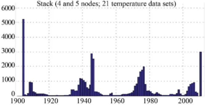
In order to get a further idea of the robustness of in- ferences that can be made from Figure 2, we have re- sumed the same computations as in Figure 2(a) (5 seg- ments, 4 nodes) for all 21 datasets that can be obtained from the CRU site

http://www.cru.uea.ac.uk/cru/data/temperature/#datter (i.e. land air temperature anomalies CRUTem3, CRU- Tem3v, CRUTem4 and CRUTem4v, sea surface temperature anomalies HadSST2 and combined land and marine temperatures HadCRUT3 and HadCRU3v, each with hemispheric means for the northern and southern hemispheres and combined global series), and we have stacked all corresponding histograms, resulting in Figure 3. There is a prominent bimodal cluster of nodes at 1938-1940 and 1945-1946 and a single mode cluster at 1975-1976, and two lesser bimodal clusters around 1904/1908 and 2006/ 2010. Altogether, most data series are well fit by a se- quence of 3 linear segments between the early 1900s and the early 2000s, with suggestions for an earlier and a later segment that remain to be confirmed.

4. Comparing Trends in Global

Temperature and the PDO and AMO

Oceanic Indices

We have applied the same method to an oceanic proxy, the Pacific Decadal Oscillation (PDO is the leading prin- cipal component of monthly sea surface temperature anomalies in the North Pacific Ocean, poleward of 20˚N). The optimal number of segments is 6 (Figure 2(c)). Two pro- minent doublets of nodes separated by ~33 years are seen, one at ~1940 and ~1948, the other at ~1973 and ~1982. A less prominent node is located at ~1919 (29 years

Figure 3. A stack of histograms calculated in the manner of Figure 2(a) with 4 nodes and 5 segments for 21 data sets from site

http://www.cru.uea.ac.uk/cru/data/temperature/#datter: land air temperature anomalies CRUTEM3, CRUTEM3v, CRUTEM4 and CRUTEM4v, sea surface temperature anomalies HadSST2 and combined land and marine tem- peratures HadCRUT3 and HadCRU3v, each with hemi- spheric means for the northern (NH) and southern (SH) hemispheres and combined global series (GL). v stands for “variance adjusted”.

before the 1948 cluster).

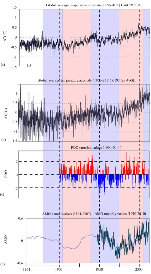
The fitting exercises above suggest a comparison, which is illustrated in Figures 4(b) and (c), where the monthly values of PDO and global temperature anomaly are shown on the same time scale. Periods when the multi-decadal slopes of linear segments fitted to the tem- perature data, as outlined in Figures 2 and 3, were po- sitive and negative have been colored, respectively, in pale red and blue. There appears to be a strong correla- tion between the sign of the slope of T (i.e. its multi- decadal time derivative) and the dominant sign of PDO. There is good correspondence between the ~1940 and ~1974 nodes of CRUTem4vGL and the main changes in PDO sign, with PDO shifting from mainly positive (between ~1930 and ~1940) to mainly negative (between ~1950 and ~1976), then back to mainly positive (between ~1976 and ~2000).

The Atlantic Multidecadal Oscillation index (AMO cha- racterizes the average sea surface temperature over the northern Atlantic; it is defined as the SST averaged over 0˚N - 60˚N, 0˚W - 80˚W, minus SST averaged over 60˚S - 60˚N) also correlates well with global mean surface temperature anomalies (as for instance already pointed out by [8]), and therefore also with the dominant multi- decadal sign changes of PDO, as seen in Figure 4(d): a decreasing linear segment prior to ~1920, an increasing one from ~1920 to ~1940, a decreasing one from ~1950 to ~1975, an increasing one after ~1975, generating a strong “~60-yr oscillation”.

5. Discussion

The above analysis suggests the possibility of causal links between some multi-decadal (~60-yr) changes in

(6)

Figure 4. (a) Monthly global average temperature anomaly HadCRUT3GL 1850-2011; (b) Monthly global average tempera- ture anomaly CRUTem4vGL 1850-2011; (c) Monthly values of PDO index 1900-2011 (positive in red, negative in blue); (d) Monthly values of AMO index 1900-2010 and annual values 1861-2007. Vertical bands shaded in pale red (respectively blue) emphasize the correlation between periods of linearly increasing (resp. decreasing) temperature, dominantly positive (resp.

egative) PDO index and increasing (resp. decreasing) AMO (see text). n

(7)

V. COURTILLOT ET AL. 369 oceanic indices PDO (and AMO) and in global surface

temperature since the early 20th century, more precisely a causal connection between changes in the modes of oceanic circulation and changes in multi-decadal (linear) trends of global surface temperature. Given the respec- tive masses, impedances and time constants involved, it is reasonable to argue that the oceanic system forces the atmospheric system on these time scales rather than the opposite.

Tsonis et al. [6] have proposed a dynamical system approach of major climate shifts, such as the ones identified by the nodes at ~1940 and ~1974. These authors define a network of oceanic indices (PDO, the El Nino Southern Oscillation ENSO, the North Atlantic Oscilla- tion NAO and the North Pacific Oscillation NPO). They find that over the period 1900-2000, this network synchronized several times. [6] define the coupling strength between indices and find that “where the synchronous state was followed by a steady increase in the coupling strength (···), the previous synchronous state was de- stroyed, after which a new climate state emerged”. The dates of the events they find are near 1910, 1940 and 1975, i.e. essentially identical (given data variance and uncertainties in node locations) to the dates we have identified for CRUTem4vGL temperature anomalies and also most other temperature data sets (Figure 3).

[6] find the same features in models of “systems with nonlinear coupled oscillators, caused by bifurcations as the coupling parameter changes”. They cannot conclude (nor can we) whether changes are triggered by some external forcing or are generated within the chaotic system itself. Their figure 2(d) illustrates the shifts in the global-SST ENSO index: this is in essence the same “box- car” correlation that can be observed in our Figure 4 be- tween T and PDO; in the present paper, we believe we provide stronger and more quantitative observational evidence of the reality of these shifts and when they occur.

A recent (~2006) shift of the temperature anomaly slope is suggested by Figures 2 and 3. In the early 2000s, the PDO turned back to a negative-dominated mode (Fig-

ure 4(c)) and the slope of the multidecadal linear trend in

AMO may have become flat, as had happened towards the end of the ~1920-1940 episode (Figure 4(d)). Also, the succession of ~30 yr long quasi-linear segments in the temperature anomaly curve (Figure 4(b): possibly 1860-1880 (?) and 1880-1910 (?), then 1910-1940, 1940- 1970 and 1970-2000) could itself suggest that the ~60 yr oscillation, whatever its source, may continue as a ~2000- 2030 segment.

We point out the puzzling fact that an earlier CRU global temperature dataset, HadCRUT3GL, displayed the alternating segments better than the latest version CRU- Tem4vGL (Figures 4(a) vs (b)). The annual variability

of the monthly averages increased by a factor of 2 in the recent revision. So did the amplitude of the temperature anomaly since 1975, that changed from 0.5 K to about 1.0 K. The segment with negative slope prior to ~1910- 1920, and more importantly the segment with flat or even negative slope after 2000, are particularly conspicuous on HadCRUT3GL (Figure 4(a)). [8] discuss the fact that the four available global temperature anomaly curves start diverging in the past two decades (their Figure 8): there is close agreement from 1900 to the late 1980s, but after that GISS and HadCRU display a plateau, whereas the NOAA and BEST curves continue to rise to values that are 0.25 K above the GISS and HadCRU plateau. It is awkward that it is the most recent part of the data compilation that displays this divergence. The plateau after the late 1990s has been the topic of much recent discussion; the previous HadCRUT3 data display this plateau much more clearly than CRUTem4vGL that seems to have suppressed it.

The shift in dominant sign of PDO (Figure 4(c)), the flattening in AMO (Figure 4(d)), and the plateau in sev- eral global temperature anomaly data (e.g. Figure 4(a)) taken together would support the hypothesis of a regime change having occurred near the end of the 20th century or early in the 21st century. A ~2000 regime change would complement the series of events at ~30-yr intervals (~1910-1920, ~1940, ~1970, ~2000). This change, if real, could imply that a ~15 year long period with no further warming lies ahead. Klyashtorin and Lyubushin [2], de Jager and Duhau [18], Scafetta [3] and Russell et

al. [19] are among several authors who have suggested

decades of future cooling: these authors argue for external forcings due to solar or planetary effects (see also the recent paper by [20]), when the mechanism of [6] en- visions the chaotic result of interaction between oceanic non-linear dynamical systems. Tsonis et al. [6] conclude that the 1970 to 2000 warming may not be (wholly) due to the radiative effect of greenhouse gases overcoming shortwave reflection effects due to aerosols and that the climate may indeed have shifted to a different state.

Our analysis strongly argues for the presence of a ~60- yr oscillation in the climate system (at least over the limited time interval—100 to 150 years—covered by relia- ble instrumental observations). More precisely, global temperature data can be interpreted as a series of linear segments interrupted by rather fast changes in slope, i.e. abrupt changes in regimes. Each episode or regime main- tains itself for approximately 30 years. We favor the oceanic system as a driver of atmospheric temperatures on these multi-decadal time scales. It remains to be seen whether abrupt changes in climate mode are a result of internal chaotic dynamics of the ocean system only or could be forced by external factors.

(8)

6. Acknowledgements

We acknowledge financial support from IPGP as part of the IEPT RAS-IPGP cooperation. IPGP Contribution NS 3391.

REFERENCES

[1] C. Essex, R. McKitrick and B. Andresen, “Does a Global Temperature Exist?” Journal of Non-Equilibrium Ther-

modynamics, Vol. 32, No. 1, 2007, pp. 1-27.

doi:10.1515/JNETDY.2007.001

[2] L. B. Klyashtorin and A. A. Lyubushin, “On the Coher- ence between Dynamics of the World Fuel Consumption and Global Temperature Anomaly,” Energy and Envi-

ronment, Vol. 14, No. 6, 2003, pp. 773-782.

doi:10.1260/095830503322793641

[3] N. Scafetta, “Empirical Evidence for a Celestial Origin of the Climate Oscillations and Its Implications,” Journal of

Atmospheric and Solar-Terrestrial Physics, Vol. 72, No.

13, 2010, pp. 951-970. doi:10.1016/j.jastp.2010.04.015 [4] J. L. Lean and D. H. Rind, “How Natural and Anthropo-

genic Influences Alter Global and Regional Surface Tem- peratures: 1889 to 2006,” Geophysical Research Letters, Vol. 35, No. 18, 2008, Article ID: L18701.

doi:10.1029/2008GL034864

[5] J. L. Lean and D. H. Rind, “How Will Earth’s Surface Temperature Change in Future Decades?” Geophysical Re-

search Letters, Vol. 36, No. 15, 2009, Article ID: L15708.

doi:10.1029/2009GL038932

[6] A. A. Tsonis, K. Swanson and S. Kravtsov, “A New Dy- namical Mechanism for Major Climate Shifts,” Geophy-

sical Research Letters, Vol. 34, 2007, Article ID: L13705.

doi:10.1029/2007GL030288

[7] P. D. Jones, D. H. Lister, T. J. Osborn, C. Harpham, M. Salmon and C. P. Morice, “Hemispheric and Large-Scale Land Surface Air Temperature Variations: An Extensive Revision and an Update to 2010,” Journal of Geophysical

Research, Vol. 16, No. 1, 2012, pp. 206-223.

[8] R. Rohde, J. Curry, D. Groom, R. Jacobsen, R. A. Muller, S. Perlmutter, A. Rosenfeld, C. Wickham and J. Wurtele, “Berkeley Earth Temperature Averaging Process,” 2011. http://berkeleyearth.org/available-resources/

[9] H. Theil, “Economic Forecasts and Policy,” North Hol- land, Amsterdam, 1961.

[10] H. J. Lüdecke, R. Link and F. K. Ewert, “How Natural Is the Recent Centennial Warming? An Analysis of 2249 Surface Temperature Records,” International Journal of

Modern Physics, Vol. 22, No. 10, 2011, pp. 1139-1159.

doi:10.1142/S0129183111016798

[11] K. L. Swanson and A. A. Tsonis, “Has the Climate Re- cently Shifted?” Geophysical Research Letters, Vol. 36, 2009, Article ID: L06711. doi:10.1029/2008GL037022 [12] I. A. Eckley, P. Fearnhead and R. Killick, “Analysis of

Change-Point Models,” In: D. Barber, A. Taylan Cemgil and S. Chiappa, Eds., Bayesian Time Series Models, Cam- bridge University Press, Cambridge, 2011.

doi:10.1017/CBO9780511984679.011

[13] K. Vasko and H. Toivonen, “Estimating the Number of Segments in Time Series Data Using Permutation Tests,”

The 2002 IEEE International Conference on Data Mining

(ICDM’02), Maebashi City, December 2002, pp. 466-473. [14] S. Kirkpatrick, C. D. Gelatt Jr. and M. P. Vecchi, “Opti-

mization by Simulated Annealing,” Science, Vol. 220, No. 4598, 1983, pp. 671-680.

doi:10.1126/science.220.4598.671

[15] G. Bhanot, “The Metropolis Algorithm,” Reports on Pro-

gress in Physics, Vol. 51, No. 3, 1988, pp. 429-457.

doi:10.1088/0034-4885/51/3/003

[16] W. H. Press, S. A. Teukolsky, W. T. Vetterling and B. P. Flannery, “Section 10.12. Simulated Annealing Meth- ods,” In: Numerical Recipes: The Art of Scientific Com-

putting, 3rd Edition, Cambridge University Press, New

York, 2007.

[17] D. Gibert and J.-L. Le Mouël, “Inversion of Polar Motion Data: Chandler Wobble, Phase Jumps, and Geomagnetic Jerks,” Journal of Geophysical Research, Vol. 113, 2008, Article ID: B10405. doi:10.1029/2008JB005700

[18] C. de Jager and S. Duhau, “Forecasting the Parameters of Sunspot Cycle 24 and Beyond,” Journal of Atmospheric

and Solar-Terrestrial Physics, Vol. 71, No. 2, 2009, pp.

239-245. doi:10.1016/j.jastp.2008.11.006

[19] C. T. Russell, J. G. Luhmann and L. K. Jian, “How Un- precedented a Solar Minimum?” Reviews of Geophysics, Vol. 48, 2004, Article ID: RG2004.

[20] J. A. Abreu, J. Beer, A. Ferriz-Mas, K. G. McCracken and F. Steinhilber, “Is There a Planetary Influence on So- lar Activity?” Astronomy & Astrophysics, Vol. 548, 2012, Article ID: A88. doi:10.1051/0004-6361/201219997

(9)

V. COURTILLOT ET AL. 371

Appendix

In order to generate broken-line models that fit the data, we have constructed an algorithm that uses two im- bricated loops.

The first, internal, loop uses the Metropolis algorithm (e.g. [16]), that generates a suite of models distributed according to a given probability law p. At iteration n the model m(n) has probability p(n). This is perturbed (see below) in order to test a new model m(test) with probability p(test). The new model is accepted if p(test) ≥ p(n) and becomes m(n + 1), replacing m(n); if p(test) <

p(n) the model is accepted with probability p(test)/p(n).

The perturbation from one step to the next is done in the following way. If N is the (given) number of segments in the broken line to be fitted to the data, there are N − 1 free nodes (the ends being assumed fixed in ab- scissa, i.e. time, not in ordinate). In an individual cal- culation, the positions of the N − 1 nodes are first drawn by assuming each node to be uniformly distributed on the full data interval. The N + 1 ordinates that define the best fit broken line (model m(1)) to the data are then cal- culated and the misfit evaluated. One of the N − 1 nodes is then selected at random and replaced by a new node with uniform probability over the data interval, and the fitting process is carried out again. This is repeated a large number of times, generating a large suite of models distributed following probability p. There are many mo-

dels where p is large, few where p is small. Residuals to the fit are modeled as a generalized Gaussian statistics, from which the model posterior probability p is derived.

The second, external loop is that of simulated annealing. The Metropolis algorithm is run with a control parameter α (see below) that slowly transforms the a po- steriori probability distribution exp(log(p)/α) from a uni- form law (in principle α = ∞) to the desired a posteriori law (α = 1). It allows convergence of the models towards regions of maximum probability. The acceptance criter- ion for a new model becomes [p(test)/ p(n)]1/α_.

In practice, in this paper, the process was iterated 300 times (inner loop), for each value of the control parame- ter α. The process was repeated starting with the final model of the previous (inner) loop, with a new, decreased value of the control parameter 0.98α (external loop). This was done starting with α = 0.1 and decreasing it to α = 0.001, i.e. about 350 steps (values of α less than 1 are due to the fact that probabilities are not normalized). This is what allows the model to escape from secondary minima. The process described above provides one “optimized” model fit, which is based on some 100,000 cal- culations. The whole process is repeated 500 times, with a new drawing of the N − 1 free nodes each time, to yield finally 500 “optimized” broken-line fits with N − 1 free nodes. Histograms of the node dates can then easily be calculated from this set.