HAL Id: tel-02171720
https://tel.archives-ouvertes.fr/tel-02171720
Submitted on 3 Jul 2019HAL is a multi-disciplinary open access archive for the deposit and dissemination of sci-entific research documents, whether they are pub-lished or not. The documents may come from teaching and research institutions in France or abroad, or from public or private research centers.
L’archive ouverte pluridisciplinaire HAL, est destinée au dépôt et à la diffusion de documents scientifiques de niveau recherche, publiés ou non, émanant des établissements d’enseignement et de recherche français ou étrangers, des laboratoires publics ou privés.
Variations atmosphériques du CO2 à l’échelle millénaire
durant le stade isotopique MIS 6
Jinhwa Shin
To cite this version:
Jinhwa Shin. Variations atmosphériques du CO2 à l’échelle millénaire durant le stade isotopique MIS 6. Sciences de la Terre. Université Grenoble Alpes, 2019. Français. �NNT : 2019GREAU006�. �tel-02171720�
THÈSE
Pour obtenir le grade de
DOCTEUR DE LA COMMUNAUTE UNIVERSITE
GRENOBLE ALPES
Spécialité : Sciences de la Terre, de l'Univers et de l'environnement
Arrêté ministériel : 25 mai 2016
Présentée par
Jinhwa SHIN
Thèse dirigée par Jérôme CHAPPELLAZ
codirigée par Roberto GRILLI et Frédéric PARRENIN préparée au sein du L’Institut des Géosciences de l’Environnement dans l'École Doctorale Terre Univers Environnement
Millennial-scale atmospheric
CO
2
variations during the
Marine Isotope Stage 6
Thèse soutenue publiquement le 18 mars 2019, devant le jury composé de :
M. Didier SWINGEDOUW
Charge de Recherches, CNRS, EPOC (Rapporteur)
M. Eric WOLFF
Professor, University of Cambridge (Rapporteur)
Mme. Pascale BRACONNOT
Directeur de Recherche, CNRS, LSCE (Examinateur)
M. Fabien ARNAUD
Directeur de recherche, CNRS, EDYTEM (Président du jury)
M. Frédéric PARRENIN
Directeur de recherche, CNRS, IGE (co-Directeur de thèse)
M. Roberto GRILLI
Charge de Recherches, CNRS, IGE (co-Directeur de thèse)
M. Jérôme CHAPPELLAZ
I
Résumé
Le dioxyde de carbone est le second gaz à effet de serre le plus abondant dans l’atmosphère après la vapeur d’eau. A cause de l’augmentation continue des concentrations de dioxyde de carbone atmosphérique due aux activités humaines depuis la révolution industrielle, prédire les changements futurs du climat et des écosystèmes est de première importance. Cependant, les prédictions exactes du climat futur sont limitées du fait des incertitudes dans les estimations d’émissions de carbone et du fait d’une connaissance imparfaite des rétroactions climat / cycle du carbone (Friedlingstein et al., 2006). En général, le CO2 atmosphérique est contrôlé par les échanges gazeux avec les réservoirs océaniques
et les stocks de carbone terrestre (Ahn and Brook, 2014; Bereiter, 2012; Landais et al., 2013). Cependant, du fait de caractéristiques différentes des réservoirs, les échelles de temps des échanges gazeux entre l’atmosphère et les stocks océaniques et terrestres sont différentes. Notre compréhension des mécanismes exacts du cycle du carbone est encore limitée, spécialement sur les échelles de temps longues.
L’objectif principal de cette thèse était de comprendre la variabilité millénaire du CO2
atmosphérique durant le stade isotopique marin 6 (Marine Isotope Stage 6, MIS 6), l’avant dernière période glaciaire (185-135 ka BP). Durant la première partie de la période MIS 6 (185-160 ka BP), 6 oscillations climatiques millénaires peuvent être observées dans des indicateurs de la température antarctique, du phénomène de bascule bipolaire dans la région Atlantique Nord et de l’intensité des moussons des basses latitudes. Un cycle hydrologique intensifié et des vêlages d’iceberg dans l’Atlantique Nord pourraient avoir impacté la circulation atlantique méridionale de retournement (Atlantic Meridional Overturning Circulation, AMOC) durant MIS 6 (Margari et al., 2010). La reconstruction de CO2 atmosphérique à partir des carottes antarctiques peut fournir des informations
clés sur le lien entre CO2 atmosphérique et variabilité climatique millénaire. Cependant, les
enregistrements existants du CO2 à partir de la carotte de glace de Vostok ne montrent pas de variabilité
millénaire du fait de trop mauvaises résolution et précision.
Pour comprendre la variabilité du CO2 atmosphérique pendant MIS 6, une précision meilleure
que 2 ppm est nécessaire, parce qu’il y a la possibilité d’observer des variations de CO2 de moins de 5
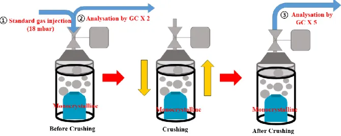
ppm pendant les plus petits événements isotopiques maximums en Antarctique (Antarctic Isotope Maxima, AIM) comme observés durant la dernière période glaciaire (Ahn and Brook, 2014; Bereiter et al., 2012). Pendant la première année de cette thèse, nous avons amélioré la précision de la méthode d’extraction existante, menant à une reproductibilité des mesures d’environ 1 ppm (1σ) lorsqu’elle est couplée avec l’analyse chromatographique des gaz (gas chromatography, GC). Cependant, en utilisant le broyeur à billes, quelques morceaux de glace relativement gros (visibles à l’oeil nu) subsistent, ce qui montre que l’efficacité de l’extraction n’est pas optimale. C’est pourquoi nous avons développé un
II
nouvel instrument appelé « système de broyage par anneaux » pour améliorer l’efficacité de l’extraction de l’air en utilisant des anneaux métalliques. Cependant, la précision du système de broyage par anneaux est 2 ppm, ce qui est moins bon que le système de broyage par billes. Nous avons donc choisi le système de broyage par billes pour reconstruire les données de CO2 atmosphérique.
Pour examiner comment le CO2 atmosphérique est lié avec le changement climatique sur les
échelles de temps millénaires pendant le MIS 6, nous avons analysé 150 échantillons de CO2
atmosphérique obtenus à partir de la carotte EPICA Dome C (EDC) sur la période 189.4-135.4 ka BP. Une oscillation mineure et 5 oscillations majeures du CO2 atmosphérique pendant la première partie de
la période du MIS 6 (189-160 ka BP) ont été découvertes. Cette variabilité est très liée avec la température antarctique. Pendant les périodes stadiales courtes dans l’Atlantique Nord, les variations de CO2 atmosphérique sont négligeables et découplées avec la variabilité de la température antarctique.
Durant ces périodes, la force de l’upwelling dans l’océan austral pourrait ne par être suffisante pour impacter le CO2 atmosphérique. De plus, 2 modes de variations du CO2 sont présentes pendant la
période du MIS 6. Le maximum de dioxyde de carbone 6 (carbon dioxide maxima 6, CDM 6) suit le réchauffement rapide de l’hémisphère Nord de seulement 100±360 ans, alors que les retards pour les CDM 3 et 4 sont bien plus longs, 1 100±280 ans en moyenne. Ces deux modes de variation du CO2
pourraient être liés à un changement de mode de l’AMOC de la première partie du MIS 6 au MIS 6e. Ces deux phénomènes sont aussi observés pendant la dernière période glaciaire. Cependant, les données disponibles permettent seulement une discussion exploratoire des mécanismes responsables de la variabilité du CO2 pendant MIS 6. Comme les conditions aux limites de la dernière période glaciaire ne
peuvent pas être appliquées au MIS 6, des données supplémentaires et des études par modélisation du MIS 6 sont nécessaires.
III
Abstract
Carbon dioxide is the second most abundant greenhouse gas in the atmosphere after water vapour. Due to the continual increase of atmospheric carbon dioxide concentration caused by human activities since the industrial revolution, predicting future climate and ecosystem changes is of increasing importance. However, exact predictions for future climate are limited because of uncertainties in estimated carbon emissions and poor knowledge about climate-carbon cycle feedbacks (Friedlingstein et al., 2006). In general, atmospheric CO2 is controlled by gas exchanges with oceanic
reservoirs and terrestrial carbon stocks (Ahn and Brook, 2014; Bereiter, 2012; Landais et al., 2013). However, due to the different characteristics of the reservoirs, the time scales of gas exchanges are different. Our understanding of the exact mechanisms of the carbon cycle is still limited, especially on longer time scales.
The main objective of this thesis is to understand the millennial variability of atmospheric CO2
during the Marine Isotope Stage 6 (MIS 6), the penultimate glacial, period (185─135 kyr BP). During the early MIS 6 period (185-160 kyr BP), 6 millennial-scale climate oscillations can be observed in proxy records of Antarctic temperature, the bipolar see-saw phenomenon in the North Atlantic region, and Monsoon intensity in low latitudes. An intensified hydrological cycle and iceberg calving in the North Atlantic may have impacted on the Atlantic Meridional Overturning Circulation during MIS 6 (Margari et al., 2010). Atmospheric CO2 reconstructions from Antarctic ice cores can provide key
information on how atmospheric CO2 concentrations are linked to millennial-scale climate changes.
However, existing CO2 records from the Vostok ice core do not show the millennial variability due to
the lack of suitable temporal resolution and precision. To understand atmospheric CO2 variability during
MIS 6, a precision of less than 2 ppm is mandatory, because there is a possibility that we could observe small CO2 variability of less than 5 ppm during the smaller Antarctic isotope maxima events as observed
during the last glacial period (Ahn and Brook, 2014; Bereiter et al., 2012).
During the first year of this PhD, we improved the precision of the existing extraction method showing a measurement reproducibility of about 1 ppm (1σ) when coupled with the GC analysis. However, using the ball mill, a few large pieces of ice (visible by eye) were still left after crushing, which shows that the air extraction efficiency was still low. Thus, we developed a new instrument called the ring mill system to improve the extraction efficiency, using metallic rings. The precision of the ring mill system, however, is ~2 ppm, which is not better than the ball mill system. Therefore, we chose the ball mill system to reconstruct atmospheric CO2 data.
To investigate how atmospheric CO2 is related with climate change on millennial time scales
during MIS 6, we reconstructed 150 samples of atmospheric CO2 data from the EPICA Dome C (EDC)
IV
atmospheric CO2 during the early MIS 6 period (189─160 kyr BP) were found. These variabilities are
highly matched with Antarctic temperature. During the short stadials in the North Atlantic, atmospheric CO2 variations are negligible and decoupled with temperature variations in Dome C. During this period,
the strength of upwelling in the southern ocean might not be sufficient to impact on atmospheric CO2.
In addition, 2 modes of CO2 variations are present in the MIS 6 period. One, corresponding to the
earliest part of MIS 6 at around 181.5±0.2 kyr BP, where carbon dioxide maxima (CDM) 6 lags abrupt warming in the Northern Hemisphere by only 100±360 yrs, and the other one, for CDM 3 (169.7±0.2 kyr BP) and CDM 4 (174.5±0.2 kyr BP) where the lag is much longer, 1,100±280 yrs on average. Theses 2 modes of CO2 variations might be related with a mode change of AMOC from the earliest
MIS 6 to MIS 6e. These two phenomena also are observed during the last glacial period. However, the limited available proxy data permit only an exploratory discussion of the mechanisms responsible for CO2 variability during MIS 6. Because the boundary conditions of the last glacial period cannot be
applied to MIS 6, additional proxy data and multiple modelling studies conducted during MIS 6 period are needed.
V
List of Abbreviations
AABW AIM AMOC BCTZ BIC CDM CIM COD DIC EDC EDML EV FID GC LID MIS NADW NH NIPR NOAA NPDW OSU P SHAntarctic Bottom Water Antarctic Isotope Maxima
Atlantic Meridional Overturning Circulation Bubble-Clathrate Transformation Zone Byrd ice core
Carbon dioxide maxima Centrifugal Ice Microtome Close-off Depth
Dissolved Inorganic Carbon EPICA Dome C
EPICA Dronning Maud Land Electronic Valve
Flame Ionization Detector Gas chromatography Lock-In Depth Marine Isotope Stage North Atlantic Deep Water Northern Hemisphere
Japanese National Institute of Polar Research National Oceanic and Atmospheric Administration North Pacific Deep Water
Oregon State University pressure gauges
VI
SNU Seoul National University
SWW Southern Westerly Winds
TCD Thermal Conductivity Detector
THC Thermohaline circulation
UBern University of Bern
VII
Table of Contents
Résumé ... I Abstract ... III List of Abbreviations ... V Chapter 1. Introduction ... 11.1. Climate and carbon cycle ... 2
1.2. Major Carbon reservoirs ... 3
1.2.1. Atmosphere ... 4
1.2.2. Terrestrial Biosphere ... 4
1.2.3. Oceans ... 5
1.2.3.1. Physical-chemical processes ... 5
1.2.3.2. The marine carbon pumps ... 6
1.2.3.3. Thermohaline circulation and CO2 cycle ... 7
1.3. Atmospheric CO2 from the ice core in the past ... 8
1.4. Carbon cycle mechanisms in the past on millennial time scales ... 10
1.5. Thesis overview ... 11
Chapter 2. The ice core archive ... 14
2.1. Sample selection for this study ... 15
2.2. Gas trapping in the ice ... 16
2.3. Physical and chemical processes affecting atmospheric CO2 signal ... 18
2.3.1. Physical processes in the firn column affecting CO2 value ... 18
2.3.1.1. Gravitational fractionation effect ... 18
2.3.1.2. Signal attenuation effect ... 19
2.3.1.3. Thermal diffusion effect ... 20
VIII
2.3.2. Chemical processes affecting gas composition in ice ... 21
2.3.2.1. Oxidation of organic molecules ... 21
2.3.2.2. The reaction of carbonate dust with acid in the ice ... 22
2.3.2.3. The snow melting-refreezing process ... 22
2.3.2.4. Antarctic ice cores for CO2 studies ... 22
2.4. Gas age calculation challenge ... 23
Chapter 3. Introduction to gas extraction methods ... 24
3.1. Wet extraction ... 24
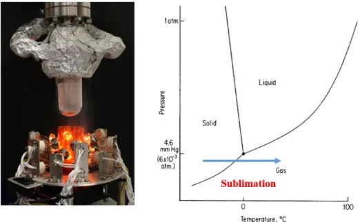
3.2. Sublimation system ... 26
3.3. Dry extraction ... 27
3.3.1. Ball mill ... 27
3.3.2. Needle cracker ... 28
3.3.3. Centrifugal Ice Microtome (CIM) ... 29
3.3.4. Drawbacks of dry gas extraction ... 30
3.4. Application of extraction methods on different ice types ... 30
Chapter 4. Improvement in the precision of the existing extraction method: the ball mill system ... 34
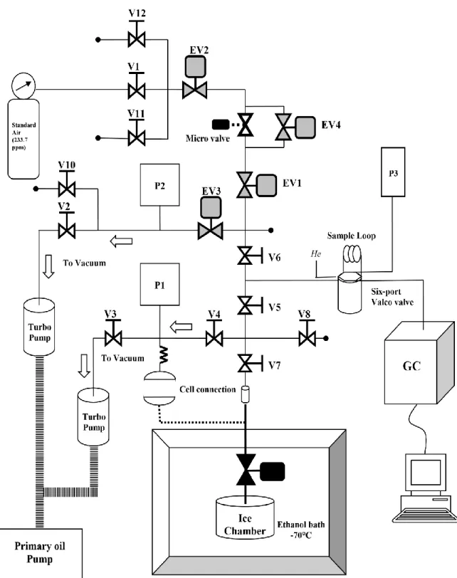
4.1. Ball mill system and Gas chromatography analysis ... 34
4.1.1. The dry extraction ... 36
4.1.2. The analytical line system ... 36
4.2. Experimental procedure ... 40
4.2.1. Cell Preparation ... 40
4.2.2. Sample preparation ... 41
4.2.3. Gas extraction ... 42
4.2.4. Blank tests ... 43
IX
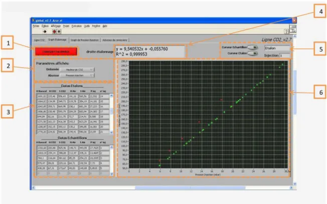
4.2.5.1. Calibration ... 44
4.2.5.2. CO2 calculation ... 45
4.2.5.3. Water vapour percentage calculation ... 45
4.2.5.4. Data correction ... 46
4.3. Improvements with respect to the existing setup ... 47
4.3.1. Reduction of water vapour inputs ... 48
4.3.2. Improvement of sample throughput ... 50
4.4. Conclusion ... 50
Chapter 5. A new high efficiency dry extraction technique for the measurement of atmospheric CO2 in Antarctic ice cores ... 51
5.1. The Ring mill system ... 52
5.2. Distribution of grain size of the ice powder ... 53
5.3. Results and discussion ... 56
5.3.1. Results from blank tests ... 56
5.3.2. Results from Antarctic ice cores ... 59
5.4. Conclusion ... 60
Chapter 6. Millennial-scale atmospheric CO2 variations during MIS 6 period ... 62
Abstract ... 63 6.1. Introduction ... 64 6.2. Methods... 67 6.2.1. CO2 measurements ... 67 6.2.2. CH4 measurements ... 67 6.2.3. Nitrogen isotopes ... 68
X
6.2.5. Ice age revision by estimating Δdepth from δ15N in air of ice ... 69
6.2.6. Age scale revision of MD01–2444 marine sediment record ... 71
6.3. Results ... 72
6.3.1. The new high-resolution and high precision CO2 record during MIS6 ... 72
6.3.2. Relationship between temperature in Dome C and atmospheric CO2 ... 73
6.3.3. Millennial variabilities during early MIS 6 period ... 73
6.3.4. Leads and lags between CO2 and the abrupt warming in Northern Hemisphere ... 75
6.4. Discussion ... 77
6.4.1. Atmospheric CO2 on millennial time scale ... 77
6.4.2. Why did CO2 lag the abrupt warming in NH during MIS 6e? ... 80
6.5. Conclusion ... 82 Annex I ... 84 Annex Ⅱ ... 85 Annex Ⅲ ... 87 Annex Ⅳ ... 90 Annex V ... 93 References ... 94
Chapter 7. Conclusions and future plans ... 98
References ... 100
1
Chapter 1
Introduction
Future climate and ecosystem changes due to the continual increase of atmospheric carbon dioxide concentration caused by human activities since the industrial revolution are inevitable but could be reduced through emission control. Projections for future climate are limited because of uncertainty with respect to estimated carbon emissions and a lack of exact knowledge about climate-carbon cycle feedbacks (Friedlingstein et al., 2006). Aside from anthropogenic emissions, atmospheric CO2 is mainly
controlled by gas exchange with oceanic reservoirs and terrestrial carbon stocks (Ahn and Brook, 2014; Bereiter et al., 2012; Landais et al., 2013). Due to the different characteristics of the reservoirs, the time scales of gas exchange between the atmosphere and the oceanic and terrestrial carbon stocks are different. Due to the limited duration of direct measurements of atmospheric CO2 which only started
in 1957 (Keeling, 1960), our understanding of the carbon cycle dynamics is limited on longer time scales.
Ice core studies allows to considerably extend the historical perspective by reconstructing atmospheric CO2 directly from gas preserved in polar ice sheets. This led so far to a record spanning
over 800,000 yrs (Lüthi et al., 2008; Petit et al., 1999). This record is essential to understand carbon cycle mechanisms on longer time scales. It notably shows that atmospheric CO2 closely parallels
variabilities in the ice core isotopic temperature record during the last 800,000 yrs (Fischer et al., 2010; Lorius et al., 1990; Petit et al., 1999). In this thesis, I reconstructed atmospheric CO2 concentrations
from the European Project for Ice Coring in Antarctica (EPICA) Dome C during the Marine Isotope Stage (MIS) 6 period (185 kyr BP─135 kyr BP), the penultimate glacial period, to understand the atmospheric CO2 variability on millennial time scales and to compare it with other records.
The general context about atmospheric CO2 is introduced in Chapter 1.1; the characteristics of
the three main carbon reservoirs involved on Quaternary time scales: atmosphere, ocean and terrestrial biosphere, are discussed in Chapter 1.2. Previous ice core studies about atmospheric CO2 over the last
800,000 yrs are introduced in Chapter 1.3. Carbon cycle mechanisms on millennial time scales are reviewed in Chapter 1.4, followed by the outline of this thesis.
2
1.1. Climate and carbon cycle
Carbon dioxide is the second most abundant greenhouse gas in the atmosphere after water vapour. The atmosphere receives short-wave energy from the sun, and this energy is partially absorbed by the surface of the Earth and re-emitted to the atmosphere as long-wave energy. This long-wave energy is partially absorbed and re-emitted by greenhouse gases in the atmosphere. This phenomenon is called the greenhouse effect. CO2 does not condense or precipitate in the atmosphere, and
considerably affects the radiative forcing of greenhouse gases by feedback mechanisms (Lacis et al., 2010).
Charles David Keeling began to measure atmospheric CO2 in Hawaii at the Mauna Loa
Observatory in 1958. The instrumental record of atmospheric CO2, measured continuously since
Keeling’s first measurements, is called the ‘Keeling curve’. Mean annual atmospheric CO2
concentrations measured at Mauna Loa Observatory have increased continuously from about 315 ppmv in 1958 to 406.99 ppmv when this chapter was written, as of August 2018. Atmospheric CO2
concentrations reached the 400 ppmv threshold on May 9, 2013, which was recorded at Mauna Loa Observatory (Tans and Keeling, 2017). This concentration is about 40 % higher than the preindustrial level, approximately 280 ppmv (Etheridge et al., 1996) and is unusually high, at least during the last 800 kyr (Lüthi et al., 2008). Atmospheric CO2 increases by ~1.5 ppmv on average every year. This
unprecedented increase of atmospheric CO2 is directly caused by human activities such as fossil fuel
Figure 1.1. Atmospheric CO2 concentrations observed directly at the Barrow, Mauna Loa and
American Samoa and South Pole Observatory. Data were obtaiend from Tans and Keeling. (2017) and NOAA website.
3
burning, cement production, reduced soil carbon stock by land use change, the increase of agricultural production.
Nowadays, atmospheric CO2 is measured by various observatories that form a global network,
allowing to depict regional differences and to better constrain the sources and sinks. These observatories include the well-known United States National Oceanic and Atmospheric Administration (NOAA) stations at Barrow and Mauna Loa in Northern Hemisphere (NH), and American Samoa and South Pole in Southern Hemisphere (SH) (Figure 1.1). With these data sets, we are able to observe atmospheric CO2 variations globally on various time scales from hourly to multi decadal scales over a period of 60
years. Global observations show a distinct seasonal periodicity of CO2, which is related with
photosynthesis of vegetation on land and soil respiration, themselves impacted by temperature and humidity on inter-annual time scales. The seasonal cycle of atmospheric CO2 is dominated by the
northern Hemisphere: due to higher global photosynthesis during the summer in the NH, atmospheric CO2 concentrations reach their annual minimum in November, and due to low photosynthesis in NH
winter, the concentration of atmospheric CO2 is highest in May. In addition, these observations show
that atmospheric CO2 emissions by fossil fuel occur mostly in the NH. The amplitude of the seasonal
change in the NH has been increasing for 40 years. On the other hand, the variation of the seasonal cycle in the SH is relatively smaller, because of a smaller land mass and less agriculture in SH.
1.2. Major Carbon reservoirs
Carbon can be stored in the atmosphere, the ocean, the terrestrial biosphere and in lithospheric sediments, the four main carbon reservoirs (Figure 1.2). The size of the carbon stock of each reservoir is different, varying from 600 Gt in the atmosphere to 63,000,000 Gt in the lithosphere (Holmen, 1992). On geological time scales, atmospheric CO2 is mainly controlled by the balance between volcanic
outgassing and carbon sequestration through continental weathering related with plate tectonics. On shorter time scales such as along the Quaternary era, the concentration of CO2 in the atmosphere is
controlled by gas exchange with the ocean and terrestrial carbon reservoirs, which is called the biogeochemical carbon cycle (Hain et al., 2014; Holmen, 1992; Sigman and Boyle, 2000). Atmospheric CO2 can be captured from the atmosphere via biological fixation in the land and oceans via
photosynthesis. On the other hand, on land, due to soil respiration, carbon can be released from the land into the atmosphere (Davidson et al., 2000; Mielnick and Dugas, 2000). Understanding possible evolution of gas exchange between the ocean and atmosphere, as well as changes of terrestrial carbon stocks become an important issue for understanding the future behaviour and role of atmospheric CO2.
In this section, only three reservoirs--ocean, atmosphere and terrestrial biosphere--are discussed. The time scale of carbon exchanges between lithospheric sediments and the atmosphere is over 200 Myr (Figure 1.2), making them negligible on millennial timescales.
4
1.2.1. Atmosphere
Among the three Earth surface reservoirs, atmosphere, land and ocean, the amount of CO2 is
smallest in the atmosphere, and the majority of carbon in the atmosphere exists as carbon dioxide. Thus, atmospheric CO2 responds sensitively to the variations of the global carbon cycle. About 380 – 600
PgC is stored in the atmospheric reservoir during glacial and interglacial periods, respectively, corresponding to concentrations of atmospheric CO2 during glacial and interglacial periods which
varied between 180 and 280 ppmv as measured in the ice core record (Lüthi et al., 2010). To understand how atmospheric CO2 is related with climate change, we should understand the timescales of carbon
exchange between atmospheric CO2 and the terrestrial, oceanic, and sedimentary reservoirs. The
residence time of a given species (i.e. CO2) in a reservoir (i.e. the atmosphere) is referred to as its
lifetime. The lifetimes of CO2 differ depending on the type of reservoirs from days to multi-millennia
and longer (Figure 1.2).
1.2.2. Terrestrial Biosphere
The terrestrial biosphere is divided into carbon in living vegetation, unfrozen soils, permafrost and peatlands. About 2,100 PgC is stored in the terrestrial biosphere.
Terrestrial carbon is involved with photosynthesis and respiration in plants, and with soil respiration (microbial and root respiration). Photosynthesis is affected by light and specific enzymes. Soil respiration is also called biodegradation, and atmospheric CO2 is produced by decomposition of
organic matter. These are mostly controlled by temperature and precipitation (Chae, 2011; Davidson et Figure 1.2. Global carbon cycle during the pre-industrial global carbon cycle (Holmen, 1992). Arrows indicates the direction of flux while numbers and arrows in red correspond to anthropogenic perturbations of the carbon cycle during 2002-2011 (Le Quéré et al., 2012; Sigman and Boyle, 2000).
5
al., 2000; Kim et al., 2010; Mielnick and Dugas, 2000). These processes are the biochemical photosynthesis-respiration reaction, which can be explained by a simple equation:
CO2+ H2O
Photosynthesis
⇄
Respiration
CH2O + O2
(1.1) The photosynthesis-respiration equation above shows that atmospheric CO2 is reduced by
photosynthesis, and via respiration, atmospheric CO2 is produced. The time scale of the carbon
exchange between vegetation and soils and atmosphere varies from years to decades (Holmen, 1992).
1.2.3. Oceans
3/4 of the Earth surface is occupied by oceans. Around 38,000Gt of carbon is stored in the world’s oceans, the surface ocean reservoir consists of about 700 – 900 PgC, and about 37,000 PgC is located in the deep ocean (IPCC, 2007). Carbon is exchanged between the atmosphere and the surface ocean on timescales of years to decades. Atmospheric CO2 is exchanged with carbon in the deep ocean
on millennial time scales (about 1,250 years) because carbon exchange with the deep ocean is governed by ocean circulation. Carbon is also exchanged between the surface ocean and deep ocean reservoirs, and the time scale for this exchange is about 25 years (Sigman and Boyle, 2000). Carbon is exchanged between atmosphere and ocean via physical-chemical, dynamical or biological processes. These three processes are discussed here.
1.2.3.1. Physical-chemical processes
Figure 1.3. CO2, HCO
−
3 and CO−23 in the surface ocean when temperature is 25°C, salinity is 35 ‰ and [DIC] is 2.1 mmol kg-1. Dotted line indicates pH of Modern surface seawater. This graph is from (Eggleston, 2015).
6
Atmospheric CO2 is soluble, thus atmospheric CO2 reacts with water to form dissolved CO2
and dissociate into three different inorganic forms: carbonic acid ion (H2CO3), bicarbonate ion (HCO−3),
and carbonate ion (CO−32). These three inorganic forms make together the so-called Dissolved Inorganic Carbon (DIC). CO2 +H2O 𝐾0 ⇄ H2CO3 𝐾1 ⇄ H++ HCO− 3 𝐾2 ⇄ 2H++ CO2 − 3 (1.2)
K0, K1 and K2 are the dissociation constants, which depend on sea water temperature, sea
water salinity and pressure. The concentration of dissolved inorganic carbon (DIC) in the ocean is the total of the concentrations of carbonic acid, bicarbonate and carbonate (eq. 1.3, eq. 1.4). Dissolved C O2 is also present in the oceans, negligible compared to DIC. Thus, the total DIC
concentration of sea water can be simplified to eq.1.5:
DIC = [CO2] + [HCO−3] + [CO2 −3] (1.3)
[CO2] = [CO2 (aq)] + [H2CO3] (1.4)
DIC ≈ [HCO−3] + [CO2 −3] (1.5)
Thus, the three DIC components are splitted depending on the pH or the alkalinity of water as seen in figure 1.3. Figure 1.3 shows speciation of DIC in the surface ocean when sea temperature in the ocean is 25°C, salinity is 35‰ and the amount of DIC is 2.1 mmol/kg. The majority of DIC is bicarbonate, which makes up ~ 90%, and the second is carbonate (around 10%). Dissolved CO2
constitutes less than 1%. Via this reaction, on short timescales, atmospheric CO2 is taken up by the
ocean to form DIC. The alkalinity in the deep ocean is affected on long timescales by this reaction, which changes the depth of the lysocline and impacts on the dissolution of calcium carbonate.
1.2.3.2. The marine carbon pumps
CO2 exchange between the atmosphere, the surface ocean and the deep ocean is described by
two major “pumping” mechanisms: the solubility pump and the biological pump (also referred to as the carbonate pump and the organic carbon pump, respectively) (Toggweiler et al., 2003a; Toggweiler et al., 2003b; Volk and Hoffert, 1985) (Figure 1.4)
The solubility pump is related with temperature and salinity due to the dissociation constants of the DIC. Solubility of CO2 is greater in cooler and fresh surface waters. Thus, the oceanic uptake of
atmospheric CO2 through this pumping mechanism is stronger in Polar Regions. The formation deep
water occurs in regions with high water density, precisely where surface waters are cold, thus these regions are synonymous with areas of high CO2 solubility.
7
The biological pump consists of the soft-tissue pump and the carbonate pump. The soft-tissue pump (or organic pump) is the cycling of carbon fixation by phytoplankton in the euphotic (sunlight) region during photosynthesis. The carbonate pump is the cycling of calcium carbonate (CaCO3)
produced by certain organisms as shells made of carbonate (CaCO3). Thus, for the biological pump,
light, CO2, nutrients (such as, nitrogen and phosphorous) and oligo-elements (Fe) are required. Nutrients
are a limiting factor in most oceanic regions. For example, in the Southern Ocean, biological productivity is limited due to a relatively low nutrient content, notably of iron (Marinov et al., 2008).
Regarding the organic carbon pump, phytoplankton is consumed by zooplankton (planktonic animals). The photosynthesized carbon is transformed in short-living particulates, such as skeletons or faecal particles. This organic carbon then sinks into the ocean interior if it is not demineralised by respiration. If organic carbon is demineralized, at the surface, the resulting CO2 is exchanged with the
atmosphere directly. Thus, DIC in the surface ocean is reduced by biological carbon fixation and the export of organic carbon into the deep ocean. These two mechanisms result in a decrease of pCO2 in
the surface ocean.
1.2.3.3. Thermohaline circulation and CO
2cycle
Ocean circulation is driven by density gradients, which are affected by temperature and salinity. It is referred to as thermohaline circulation (THC). Deep cold and salty waters are formed at high latitudes of both hemispheres especially in the North Atlantic region and the Southern Ocean (Figure 1.5). Deep water originating in the North Atlantic region is referred to as North Atlantic Deep Water Figure 1.4. Two major pumping mechanisms of CO2 from the atmosphere into the ocean (IPCC,
8
(NADW) and the deep water current from the Southern Ocean is referred to as the Antarctic bottom water (AABW). The Atlantic Meridional Overturning Circulation (AMOC) is composed of the Antarctic Bottom Water (AABW), making up the upper overturning cell, and North Atlantic Deep Water (NADW), which forms the lower overturning cell. The strength of AMOC is thought to play a major role in the so-called “bipolar seesaw mechanism” (Broecker, 1998; Stocker and Johnsen, 2003), corresponding to the reverse trends in the temperature records from Greenland and Antarctica during rapid climatic events of past glaciations. When temperature increases in the Northern Hemisphere, it generates ice sheet melting. The resulting meltwater partly runs toward the surface of the North Atlantic Ocean, which salinity is reduced. The density of surface water in the North Atlantic thus decreases, leading to a reduction of NADW intensity. This leads to subsequent cooling of the Northern hemisphere and warming of Antarctica. This change of ocean dynamics can impact on the carbon cycle, through mechanisms which will be discussed in detail in section 1.4.
1.3. Atmospheric CO
2from the ice core in the past
Beyond the instrumental record providing direct measurements into the atmosphere, atmospheric CO2 concentration can be reconstructed in principle via various paleoclimate records: ice
cores, the carbon isotopic composition of phytoplankton, boron isotope signatures of foraminifer shells and leaf stomata density patterns (Royer et al., 2001). However, out of these records, only polar ice cores permit us to reconstruct a precise and reliable record of atmospheric CO2 concentration in the past
(Bereiter et al., 2012; Marcott et al., 2014; Petit et al., 1999). The mechanisms leading to the formation of this paleo-record of atmospheric CO2 will be explained in section Chapter 2. The other CO2 proxies
allow a reconstruction of CO2 concentrations over much longer geological periods than ice cores,
however, the precision of the data is low.
9
Atmospheric CO2 variations and temperature derived from δD of water over the last 800,000
years are shown in Figure 1.6 (Jouzel et al., 2007; Lüthi et al., 2010; Petit et al., 1999), covering 8 glacial and interglacial cycles. During the interglacial periods, CO2 concentration varied between 250–
300 ppmv. In addition, Figure 1.6 shows that atmospheric CO2 closely parallels temperature variability
as reconstructed from EDC during that period (Fischer et al., 2010; Lorius et al., 1990; Petit et al., 1999). During glacial periods, CO2 concentrations decrease slowly to about 180 ppmv. CO2 concentrations
during the minima of glacial periods vary between 170–190 ppmv. During the glacial terminations atmospheric CO2 increases rapidly from the glacial period level to the interglacial level.
Figure 1.6. Top: Iron fluxes from EDC (Martínez‐Garcia et al., 2009). Middle: Temperature proxy data which are derived from continuous stable water isotope records. These two data were obtained from EDC and Vostok ice core (Jouzel et al., 2007; Petit et al., 1999). Bottom: Atmospheric CO2
concentrations from EDC and Vostok ice cores (Fischer et al., 1999; Lüthi et al., 2010; Monnin et al., 2001; Petit et al., 1999; Siegenthaler et al., 2005). Bold dashed lines in blue indicate a CO2 estimate
derived from the linear interpolation. Age scale of these data for the EDC and the Vostok ice cores set are on the EDC3 and GT4 age scale, respectively.
10
Millennial–scale variability of atmospheric CO2 has been carefully investigated over the last
glacial period. It appears to be closely linked to major Antarctic Isotope Maxima (AIM) (Ahn and Brook, 2014; Bereiter et al., 2012), varying on the order of 10–20 ppmv during the major AIM events (Bereiter et al., 2012). Atmospheric CO2 reaches its maximum values with a delay with respect to Antarctic
temperature. It then decreases slowly. However, this apparent offset may be related with the difficulty to accurately estimate the age offset between the ice and the trapped gases in the ice (Loulergue et al., 2008). During the smallest Antarctic isotope maxima events, smaller CO2 variabilities are observed of
less than 5 ppmv (Ahn and Brook, 2014; Bereiter et al., 2012).
1.4. Carbon cycle mechanisms in the past on millennial time scales
In general, atmospheric CO2 on millennial-timescale can be controlled by CO2 exchange
between Ocean and Atmosphere, as well as changes of terrestrial carbon stocks. Coupled climate carbon cycle models reported that the variations of atmospheric CO2 concentration on millennial-timescale are
mainly dominated by deep ocean inventory requiring a few millennia to react to climate change (Schmittner and Galbraith, 2008). These variations of CO2 concentration might be compensated by fast
changes in the terrestrial biosphere (Bouttes et al., 2011; Menviel et al., 2014; Schmittner and Galbraith, 2008).
In the deep ocean reservoir, the Southern Ocean is important in regulating global atmospheric CO2 variations on millennial time scales (Ahn and Brook, 2014; Bereiter et al., 2012). This is identified
by a close relationship between atmospheric CO2 and Antarctic temperature in EDC during the last
800,000 years (Lüthi et al., 2008). Because the Antarctic Circumpolar current in the Southern Ocean is highly enriched in dissolved CO2, CO2 can be released from the ocean to the atmosphere via Southern
Ocean ventilation, possibly driven by changes in stratification, buoyancy forcing and the strength and position of circumpolar westerly winds (Toggweiler et al., 2006) and the variations of sea ice extent in the Southern Ocean (Stephens and Keeling, 2000). Changes in the AMOC (Schmittner and Galbraith, 2008), are also thought to be important mechanisms of CO2 release into the atmosphere on millennial
time scales.
Exchange between deep and shallow waters in the Southern Ocean is partly conditioned by Southern Westerly Winds (SWW) which is a zonal circulation system located in the mid latitudes of the Southern Hemisphere. SWW moves surface waters northward by Ekman transport in the Southern Ocean. Surface waters are then replaced by the upwelling of deep water, containing high amounts of dissolved CO2. Upwelling of deep water driven by wind in the Southern Ocean can thus
release CO2 to the atmosphere (Toggweiler et al., 2006). Therefore the SWW position and strength in
the Southern Ocean can substantially impact on the upwelling and ventilation of deep water, and is a key factor for modulation of atmospheric CO2.
11
In the Southern Ocean, biological productivity is limited, reflected in a relatively low chlorophyll content. This indicates that the phytoplankton in the Southern Ocean have limited access to essential micronutrients such as iron. Aeolian dust input into the Southern Ocean can modulate iron deposition. If the amount of aeolian dust input in the Southern Ocean increases, the productivity of phytoplankton in the Southern Ocean increases and carbon fixation in the Southern Ocean biosphere is thus enhanced. Organic detritus sinks into the deep ocean reservoir (Marinov et al., 2008), and atmospheric CO2 can thus be drawn down by what is known as the biological carbon pump (Martin,
1990). Atmospheric CO2 might also be affected by sea ice dynamics, because sea ice may block the
carbon exchange between the atmosphere and the Southern Ocean (Stephens and Keeling, 2000). Sea ice can also suppress the extent of surface water where biological fixation occurs actively (Hillenbrand and Cortese, 2006). This may have an impact on the efficiency of deep-ocean internal mixing, and therefore the mean residence time of carbon in the ocean (Ferrari et al., 2014). A reduced biological pump can also increase atmospheric CO2 when upwelling of deep water with abundant nutrients is
reduced (Schmittner, 2005). Thus, the impact of upwelling in the Southern Ocean on atmospheric CO2
concentrations may have multiple, counteracting components.
The AMOC is able to control atmospheric CO2 concentrations as well (Bouttes et al., 2011;
Menviel et al., 2014; Schmittner and Galbraith, 2008). When large amounts of low-density fresh water are released into the North Atlantic, the AMOC is shut down. Thus, heat piles up in the South, and moisture movement from the Atlantic to the Pacific is reduced. Therefore, sea ice retreats in the Southern Ocean. On the other hand, the North Atlantic is cooled, and the Intertropical Convergence Zone is shifted to the south. Salinity at the surface of the Pacific Ocean is increased. Thus, AABW and North Pacific Deep Water (NPDW) transport are enhanced (Menviel et al., 2014). Enhanced NPDW transport ventilates deep Pacific carbon via the Southern Ocean. Thus, atmospheric CO2 increases.
Terrestrial carbon is affected by variation of vegetation and soil respiration (microbial and root respiration) in the terrestrial biosphere. Temperature and precipitation are the most important control factors for these two processes (Chae, 2011; Davidson et al., 2000; Kim et al., 2010; Mielnick and Dugas, 2000). Thus, thawing of permafrost (Köhler et al., 2014), biomass decomposition caused by drought which cause decomposition of biomass (Marcott et al., 2014), changes in precipitation connected to shifts of the Intertropical Convergence Zone (mainly in northern Africa and northern South America) may cause variations in terrestrial carbon stocks (Menviel et al., 2008).
1.5. Thesis overview
The main goal of this thesis is to understand atmospheric CO2 variability on millennial time
scales during the penultimate glacial period (approximately 185 to 135 kyr BP) and also to explore similarities/differences in atmospheric CO2 variations on millennial time scales during the past two
12
glacial periods. These two glacial periods are also identified by numbered Marine Isotope Stages (MIS). Marine Isotope Stages are numbered stages that were originally designed to designate the major climatic swings. The penultimate glacial corresponds to MIS 6 and the part of the last glacial period investigated in this study corresponds to the MIS 3 period (60–27 kyr BP) (Figure 1.7). To this end, I reconstructed for the first time at high temporal resolution and with a suitable analytical precision atmospheric CO2
concentrations from the EDC ice core during the MIS 6 period.
Polar ice cores permit us to directly reconstruct a record of atmospheric CO2 concentration in
the past (Bereiter et al., 2012; Marcott et al., 2014; Petit et al., 1999). However, this does not mean that all ice cores have equal potential to reconstruct CO2 concentrations. The potential of CO2 reconstruction
from Greenland and High Mountain ice cores is limited due to contamination. In addition, we cannot reconstruct CO2 concentrations over the entire 800 kyr period covered by ice cores with a sub-centennial
time resolution due to the physical processes of gas trapping in the firn layer of the ice sheet, which smooth atmospheric gas concentrations. These processes are discussed in Chapter 2.
To reconstruct atmospheric CO2 concentrations from ice cores, wet extraction (Kawamura et
al., 2003), crushing extraction (Ahn et al., 2009; Bereiter et al., 2013) or sublimation extraction (Schmitt et al., 2011) are used. In Chapter 3, different extraction techniques are described. High precision measurements are needed to observe small CO2 variability of less than 5 ppmv during the smallest
Antarctic isotope maxima events (Ahn and Brook, 2014; Bereiter et al., 2012). To understand atmospheric CO2 variability during MIS 6, a precision of less than 2 ppmv is mandatory. We improved
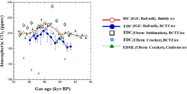
the precision of the existing extraction method – based on a ball mill - showing a measurement Figure 1.7. Atmospheric CO2 concentrations from Antarctica (Bereiter et al., 2015) and local
13
reproducibility of about 1 ppmv (1σ) when coupled with the Gas chromatography analysis. The improved procedure and how the measurement are improved are introduced in Chapter 4. However, using the ball mill, a few large pieces of ice (visible by eye) were still left after crushing, which shows that the air extraction efficiency is not optimal. Thus, we tested a new extraction method to improve the extraction efficiency, as described in Chapter 5.
In Chapter 6, new atmospheric CO2 data on millennial time scales during the penultimate glacial
period are presented. Similarities and differences between atmospheric CO2 during the past two glacial
periods are discussed. Some possible mechanisms which may be involved in atmospheric CO2
variations on millennial time scales are suggested, followed by the main conclusions of this thesis and future plans.
14
Chapter 2
The ice core archive
Polar ice cores are vertical cores obtained from the Greenland and Antarctic ice sheets, usually drilled at locations where snow accumulates annually and does not melt, in order to obtain continuous records. Deep ice cores are usually drilled at ice domes or ice divides where the ice is stratigraphically well-layered and ice sheet flow is at a minimum. When snow accumulates on a polar ice sheet, the air that circulates via the overlying layers is occluded in the ice layers directly. Thus, air initially in the form of bubbles deeper as clathrates in the ice captures the atmospheric composition when the ice formed. With ice and occluded air from ice cores from Greenland and Antarctica, we can obtain continuous information on the climate of the past that long predates direct instrumental measurement. For example, the isotopic composition (such as δ18O, δD) of the ice allows us to quantify temperature
variations in the past. Tephra produced from volcanic eruptions which occurred close to ice core sites are also deposited in in ice cores. In addition, dust and chemical aerosol species (Na+, NO−
3, NH+4) are
also recorded in the ice, which allow us to understand the changes of atmospheric circulation pattern. From the occluded air in the ice, we can reconstruct the atmospheric composition directly including the trace greenhouse gases CO2, CH4 and N2O.
The atmospheric CO2 record in ice coresreflects atmospheric CO2 in the past, but physical and
chemical properties may affect atmospheric CO2 signals. First, air is moved into the firn via diffusion
and air is trapped gradually. Gas moves into the firn column at different rates, and the heavier molecular species are enriched at the bottom of the firn, which can bias measured atmospheric CO2 concentrations.
Second, CO2 records can be contaminated by the in-situ production of CO2 caused by carbonate-acid
reactions and oxidation of organic molecules. In addition, due to the snow melting-refreezing process, CO2 data can be scattered due to higher solubility in water compared to other gases (Neftel et al., 1983).
These three processes can lead to differences between measured CO2 values and the real values of
atmospheric CO2.
In this chapter, I discuss about gas trapping in the ice and how physical and chemical properties affect atmospheric CO2 signals. In this chapter, in Chapter 2.1, we introduce ice core sites in Antarctica
that are used in this study. In Chapter 2.2, gas trapping in the ice is introduced in detail. Then, the impact of the gas trapping process on atmospheric CO2 signals in ice cores is discussed in Chapter 2.2. In
Chapter 2.3, contamination of the atmospheric CO2 signal in the firn due to physical and chemical
processes in the firn will be discussed. Finally at a given depth, ages of the air and ice are different. This will be discussed in Chapter 2.4.
15
2.1. Sample selection for this study
In this thesis, EPICA Dome C (EDC) is chosen to reconstruct atmospheric CO2 during MIS 6.
Samples from the Talos Dome ice core (TALDICE) are used to test the accuracy of a new crushing system. The locations of these ice cores are plotted in Figure 2.1 and detailed information about the drilling sites is introduced in Table 2.1. The Vostok ice core, which was previously used for CO2
reconstruction during MIS 6, is also introduced (Petit et al., 1999).
Table 2.1 Glaciological characteristic of Antarctic ice cores.
EDC Vostok TALDICE
Latitude Longitude 75°06’S, 123°21’E 78°28’S, 106°48’E 72° 47’S, 159° 04’E
Annual mean Temperature (°C) -54.5 -57.3 ─41
Accumulation rate (mm water equiv. yr-1) 28.5 22 80
Brittle zone depth (m) 600 ─ 1200 300─720 667─1002 Brittle zone ice age range (kyr BP) 29 ─ 84 13─50 12─35
Length of core (m) 3270.2 3667 1620
Age at bottom (kyr B.P.) 800 kyr 420 ky (for 3300m) 150 kyr References (Parrenin et
al., 2012; Schwander et
al., 2001)
(Petit et al., 1999) (Frezzotti et al., 2004; Schilt et al.,
2010) Figure 2.1. Location map of EDC (in red), Vostok (in blue) and TALDICE (in yellow), the three ice cores used and mentioned in this study (Dunbar and Kurbatov, 2011).
16
2.2. Gas trapping in the ice
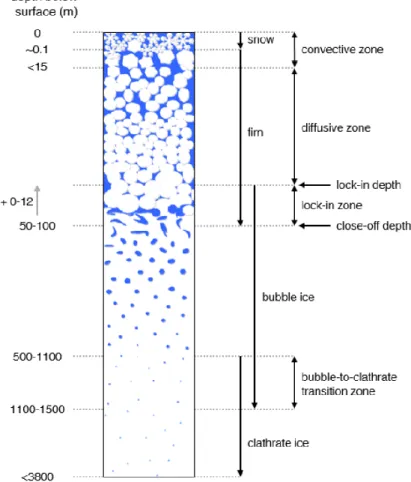
Fresh dry snow is deposited continuously on the surface in the dry snow zone of the ice sheet ice sheets i.e where no surface melting occurs. The compositional and isotopic characteristics of freshly deposited snow show annual cycles, and it is often possible to distinguish annual layers, particularly in high-accumulation areas and in the uppermost layers of snow and firn. Annual layers, however, are quickly lost due to wind-driven mixing in the low-accumulation areas of the Antarctic plateau. As snow accumulates at the sites during centuries to millennia, this accumulated powdery snow is pressed continuously under its own weight. Snow starts to compact into firn by the increase of hydrostatic pressure with depth. The snow particles become rounded and jointed together, and are thus transformed into firn (Figure 2.2). This topmost layer of the ice sheet, composed of fresh snow and low-density firn, is highly porous.
The layers of firn become denser due to dry sintering and plastic deformation. As these layers become sufficiently dense, firn becomes ice (Schwander, 1989). Figure 2.2 shows the firn densification process in a polar ice sheet. The transformation of surface snow into ice layers requires between ~100 and ~6,000 yrs (Blunier et al., 2007).
Figure 2.2. This figure shows the firn densification process and gas trapping process in the Antarctic ice sheet (Bereiter, 2012; Nehrbass-Ahles, 2017; Schwander, 1996).
17
Due to the absence of melt in cold polar ice sheets, air can move freely into the open pore space in the topmost part of the firn column via convection, and the air is moved into the deeper firn via diffusion and finally trapped in the ice sheet. This process can be divided into three zones (Sowers et al., 1992). The first zone is the convective zone, the highest position where air is well-mixed by the pressure gradient with respect to the surface (Clarke and Waddington, 1991). This zone usually reaches depths in the first 15 m (Landais et al., 2006; Severinghaus et al., 2010). The density of surface snow is 0.3─0.35g/cm3
(Bender et al., 1997), and the porosity of this zone is 62─67 %. Convection in the uppermost firn is affected by wind forcing. The depth of this zone can be determined in part by the wind speed and accumulation rate (Kawamura et al., 2006).
In the diffusive zone, the stagnant/static air column below the convective zone, air is moved into open pores by molecular diffusion. The movement of molecules is thus affected by temperature. In this zone, gases are still in contact with the atmosphere. When the density of the firn reaches ~0.815-~0.845 g/cm3 in the bottom of the diffusive zone, the diffusion effect decreases (Buizert et al., 2012). The air is trapped at this depth, which is called the lock-in depth (LID) (Schwander and Stauffer, 1984). The depth of the LID varies from 50 to more than 100m, which depends on the accumulation rate and the mean annual temperature. For example, the LID in Vostok varies on the order of 100 meters.
Below the diffusive zone is a non-diffusive zone or bubble formation zone. The height of this zone is 2~12 m, which is dependent on the seasonal snow and firn layer anisotropy. The pores between snow particles are totally isolated from each other and from the atmosphere, and form bubbles. However, additional air is occluded in pores between the lock-in depth and the close-off depth. Gas can move horizontally along permeable layers, because the firn permeability is different vertically. This interval is called the lock-in zone or pore closing zone, both of which refer to the non-diffusive transitional zone between firn and ice which is located a few meters (roughly 5-10 m) below the LID. The ice density of this zone is between 0.815-~0.845 g/cm3 (Arnaud, 1997), the volume of the air is 10-15 percent. Finally, bubbles become completely trapped in the ice at the Close-off Depth (COD) which
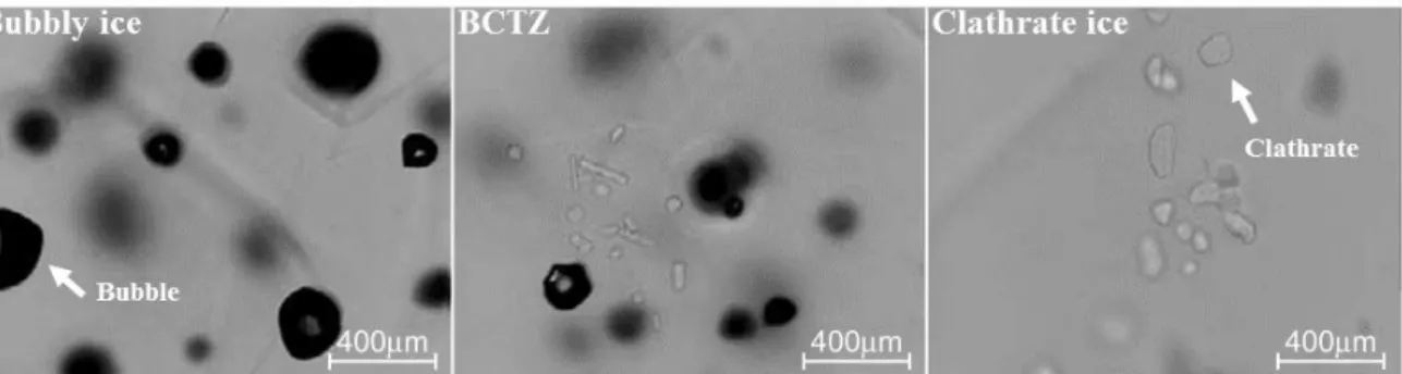
Figure 2.3. Images of air inclusions in the Dome Fuji observed under an optical microscope (Ohno et al., 2004). Left: Air bubbles above the transition zone. Middle: Bubbles and clathrates in the transition zone Right: Clathrates below the transition zone. This figure is from Ohno et al. (2004).
18
is determined by the mean surface temperature, pressure and accumulation rates, and wind speed (Kaspers et al., 2004). Bubbly ice covers only 15 % of cores in Antarctica.
Because of the hydrostatic pressure increase at depth, bubbles are compressed in the first several hundred meters in the ice sheet. They are caged in the clathrates (Figure 2.3). If hydrostatic pressure exceeds the dissociation pressure, the air bubble is pressed into the ice lattice. The air molecules are occluded in the crystalline structure of the ice, caged in an H-bonded structure. These structures are referred to as clathrates (Ohno et al., 2010; Uchida et al., 2014). Clathrates start to be formed at around 500─1100 m. At these depths between where clathrates start to form and where bubbles disappear, bubbles and clathrates exist together (Lipenkov, 2000) (Figure 2.3). This area is called the bubble-to-clathrate transition zone (BCTZ) (Lüthi et al., 2010), or gas-bubble-to-clathrate transition zone (Kobashi et al., 2008). The thickness of the BCTZ is 180─700 m (Uchida et al., 2014). In the deeper part of the BCTZ, the size of the clathrates is smaller than that of the bubbles.
2.3. Physical and chemical processes affecting atmospheric CO
2signal
2.3.1. Physical processes in the firn column affecting CO
2value
2.3.1.1. Gravitational fractionation effect
In the topmost layer in the polar ice sheet, gas is well-mixed by wind-pumping (Clarke and Waddington, 1991). The heavier molecular species are enriched in the firn bottom due to earth’s gravitational field. A gravitational fractionation effect develops with depth and mass difference between gas species (Craig et al., 1988). The gravitational fractionation effect is not related with the absolute molar mass, but rather with the difference in the masses (∆m) between two molecular species. If the height of the diffusion zone is larger, the heavier isotopes are preferentially accumulated. Thus, gravitational fractionation is highly associated with the height of the diffusion zone. The gravitational fractionation effect is therefore dependent on the temperature and accumulation rates at the site because these climate factors can impact on the firn column height. The isotopic enrichment in the LID is estimated using the barometric equation as below:
δ =[𝑅
𝑅0− 1] × 10
3= (𝑒∆𝑚𝑔𝑅𝑇 − 1) × 1000 ≅∆𝑚𝑔𝑧
𝑅𝑇 (‰) (2.1)
Where R is the ideal gas constant, ∆m is the absolute mass difference between the isotopes of the same species (kg/mol), g is the gravitational acceleration (9.82 m/s2), Z is the height of the diffusive column
19
Due to the gravitational fractionation, the heavier molecules are enriched in the firn bottom. CO2 measurement data is thus higher than real atmospheric concentrations, and the data should be
corrected. The isotopic ratio of 15N/14N of N2 and 40Ar/36Ar of in the ice can be used to estimate the
amount of gravitational fractionation effect. The δ15N isotope ratio of N
2 is constant in the atmosphere
on orbital time scales (Mariotti, 1983) but δ15N isotope ratio started to be biased from the upper part of the diffusion zone to the LID due to the gravity. In addition, the gravitational fractionation effect depends on the weight of the difference of two isotopic mass, and to estimate the enrichment of CO2
we should calculate the difference between the molar mass of atmospheric CO2 and the molar mass of
air. Considering the mean molar mass of air is ~29g/mol, which is similar to the molar mass of N2, the
isotopic enrichment is estimated using the isotopic ratio of 15N/14N of N
2 in the ice, using the equations
below:
CO2, corr = CO2, obs ─ (𝑀𝐶𝑂2─ 𝑀𝑎𝑖𝑟) × 𝛿15𝑁 × CO2, obs= CO2, obs × (1 −
𝛿15𝑁×15.2
1000 ) (2.2)
Where M is the mass of the molecular weight of species.
However, δ15N isotope ratio data is not always available for the data correction. In this case,
the δ15
N isotope ratio can be estimated using an empirical relationship between deuterium data and δ15N (Dreyfus et al., 2010; Schneider, 2011). However, this is not ideal because the relationship between temperature and δ15
N does not hold for some time periods (for example, MIS6 period in EDC). The equation commonly used to estimate δ15N from deuterium is as below:
𝛿15𝑁 = 0.0020032 × 𝛿𝐷 + 1.2969 (2.3)
2.3.1.2. Signal attenuation effect
The surface atmosphere is mixed with older air in the firn. Thus, air over decades to millennia, depending on the temperature and accumulation rate at the drilling site, is mixed in the firn layers (Schwander and Stauffer, 1984). In addition, the bubbles at a certain depth do not necessarily close at the same time. Thus, a signal of atmospheric CO2 is integrated over decades to millennia, which is
referred to as the smoothing effect, signal attenuation effect or damping effect. If the duration of the signal is shorter than the width of the gas age distribution, the CO2 signal can be smoothed out. This
20
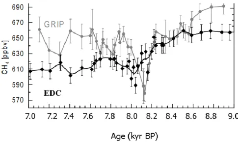
smoothing effect is mainly governed by the speed of porosity closure, which is highly related to accumulation and temperature. The smoothing effect is stronger for lower accumulation and/or lower temperature. This effect removes high-frequency signals and reduces the amplitude of the signal if the width of the gas age distribution in the site is broader. Figure 2.4 shows an example of smoothing effect. The atmospheric CH4 series from Greenland (GRIP) shows a rapid change of CH4 during the abrupt
cooling event at 8.2 kyr BP. However, the atmospheric CH4 series from EDC, which has much lower
accumulation rates with respect to the GRIP site, shows a much smaller variation. CH4 data from EPICA
Dome C (EDC) is attenuated by 34 to 59 ‰ compared to the data from GRIP.
2.3.1.3. Thermal diffusion effect
Gas movement is also subjected to thermal gradients within the diffusive zone. Heavier isotopes preferentially accumulate at the cooler part of the thermal gradient (Grachev and Severinghaus, 2003). If the temperature gradient is large, this phenomenon can be significant (Severinghaus et al., 2001). This mechanism, known as the thermal fractionation effect, is superimposed on the gravitational fractionation effect, and can be estimated using δ15N in the occluded air. The thermal fractionation effect
is described by the following equation:
𝛿𝜏 = [(𝑇 𝑇0)
𝑐
─ 1] × 1000 (2.4)
where T is the temperature at the bottom of the diffusive column, T0 is the temperature at the surface of
the diffusive column and C is the thermal diffusion coefficient. This mechanism can be important on the CO2 mole fraction for large temperature differences in the firn column. However this effect is not
21
significant on the CO2 mole fraction (Eggleston, 2015; Schneider, 2011) because temperature gradients
in interior Antarctica tend to be gradual (Jouzel et al., 2007).
2.3.1.4. Heterogeneous gas trapping
The physical characteristics of the firn column at the drilling site determine the properties of gas close off as well. Fluctuations in the density of the firn, for example, can influence close off depth. At relatively dense layers in the firn, air can be closed off earlier (Kawamura et al., 2006). Thus, some bubbles at a given layer could be enclosed earlier and at a shallower depth than the surrounding layers. In this case, the occluded air in the early close-off bubble is relatively older than those of the surrounding layers. In lower-density firn layers, bubbles can be closed off later and deeper than the bubbles in the surrounding layers, and the trapped air is thus relatively younger than air in the surrounding layers. Air is therefore not necessarily trapped in exact chronological order. This effect is thought to be larger at low accumulation sites than at higher accumulation sites (Fourteau et al., 2017). Variations in the gas trapping process can be more clearly observed when gas composition changes rapidly. This phenomenon is observed in CH4 concentrations from Vostok 4G-2 with low accumulation on cm-scale
variations at around 60 kyr BP when climate changes rapidly (Fourteau et al., 2017).
At the time of writing, no study directly addresses whether CO2 concentrations are also affected
by this mechanism. Methane concentrations vary rapidly when compared to carbon dioxide, and this effect might have a greater impact on atmospheric CH4. On the other hand, the possibility of an impact
on atmospheric CO2 concentrations cannot be ruled out. (Nehrbass-Ahles, 2017). Since the gas trapping
process can impact gas age distributions, the CO2 signal should also be affected.
2.3.2. Chemical processes affecting gas composition in ice
2.3.2.1. Oxidation of organic molecules
CO2 can be produced in the via oxidation of organic compounds (HCHO, CH3COO- and
HCOO─) by an oxidizing agent such as hydroxide peroxide (H2O2) either biologically (Campen et al.,
2003) or abiologically (Tschumi and Stauffer, 2000). The oxidation of organic molecules is described as follows:
H2O2 + H2CO → CO2 + H2 + H2O (2.5)
22
2.3.2.2. The reaction of carbonate dust with acid in the ice
CO2 concentrations can be contaminated by the in situ production of CO2 caused by
carbonate-acid reactions (Delmas et al., 1980). CaCO3 and H+ are mainly involved in this reaction. This reaction
can occur when the ice is acidic and decarbonate CaCO3 which is present in the ice as dust particles
(Smith et al., 1997a) and form CO2─3 . The carbonate and acid reaction is the reaction between CO3 2─and protons to form CO2.The reaction consists of two steps, which are described as below:
CO2 −3 + H+ ⇄ HCO3 − (2.7)
HCO3 − + H+ ⇄ CO2+H2O (2.8)
These reactions are reversible, and the direction of the reactions is determined by the equilibrium state of the components. For example, if the concentration of calcium ions (Ca2+) is higher
than 70 ppb in the ice, the corresponding carbonate formed during decarbonation reacts to neutralize the existing H+, and the overall reaction occurs as below:
CO2 + H2O + CO2 −3 → 2HCO3 − (2.9)
Due to this chemical reaction, atmospheric CO2 can be depleted in principle, however, any clear
evidence for the depletion in the ice where air is occluded in bubbles could not be found yet. However this depletion of atmospheric CO2 is observed in the BTCZ (Tschumi and Stauffer, 2000).
On the other hand, if the concentration of calcium (Ca2+) is lower than 5 ppb at the site before ice is formed, CaCO3 can react with H+, and the atmospheric CO2 concentration cannot be contaminated
in this case.
2.3.2.3.
The snow melting-refreezing processCO2 concentration can be considerably contaminated because CO2 is highly soluble in water
compared to other gases (Neftel et al., 1983). When ice is melted, atmospheric CO2 can be dissolved.
If the melted ice freezes again at the ice coring sites, this dissolved gas in the water might be trapped in the bubbles of the ice. Thus, CO2 concentrations are artificially increased. In addition, carbonate-acid
reactions can occur in the melt water (Anklin et al., 1995).
2.3.2.4.
Antarctic ice cores for CO2 studiesAtmospheric CO2 is usually reconstructed from the Antarctic ice cores because of higher
23
mentioned above, these impurities can cause carbonate-acid reaction and the oxidation of organic carbon. This can cause large scattering of atmospheric CO2 data. Some examples on CO2 production in
Greenland are as below:
CO2 records from Antarctic ice core agree with those from Greenland within age uncertainties
and analytical uncertainties during the last 300 yrs. However at the beginning of the second millennium, atmospheric CO2 concentrations reconstructed from Greenland ice cores (Eurocore and GRIP) is higher
than those from Antarctic ice core by up to 20 ppmv during the millennium. Considering the inter-hemispheric gradient effect might be between – 1 and + 5ppmv (Anklin et al., 1995), this difference might be partially related with interhemispheric gradient but it is mostly caused by chemical reaction in the ice. This is confirmed by the amount of impurities in Greenland ice and the Antarctic ice
(Barnola
et al., 1995)
. In addition, during the last glacial period, atmospheric CO2 in Greenland during theinterstadial is higher than those during the stadial by 50-90 ppmv on average (Smith et al., 1997), however this high variations during the last glacial period were not observed in Antarctic ice cores (Oeschger et al., 1988).
Thus to obtain less in situ CO2 production in ice, a low carbonate concentration and H2O2 in an
ice core are important. Luckily, Antarctic ice cores have relatively low concentrations of H2O2 and
carbonates and have low temperature compared to Greenlandic ice cores, which can reduce the risk of CO2 contamination (Tschumi and Stauffer, 2000).
2.4. Gas age calculation challenge
At equivalent depth in an ice core, the age of the air is younger than the age of the surrounding ice. Thus, ice cores have different chronologies for the air and ice phases. The difference between the age of the air and ice at a given depth is referred to as delta age (∆age); the analogous difference in depth between air and ice with the same age is referred to as delta depth (∆depth). If the gas trapping process occurs slowly, as is the case at the low-accumulation drilling sites in the Antarctic interior, ∆age is larger.
∆age is usually calculated by firn densification models which usually take into account temperature, accumulation rate, wind speed and insolation change. To improve the relative chronology between ice and gas, delta depth between gas and ice can also be calculated using δ15N data, which
reflects the height of the diffusive column. From δ15
N data, the depth difference between synchronous events in the ice matrix and gas bubbles is estimated. The uncertainties of the δ15N method are often
smaller than those of modelling or orbital wiggle-matching. In this thesis, we use a ∆age calculation to improve the chronology of
![Figure 1.3. CO 2 , HCO − 3 and CO −2 3 in the surface ocean when temperature is 25°C, salinity is 35 ‰ and [DIC] is 2.1 mmol kg -1](https://thumb-eu.123doks.com/thumbv2/123doknet/14713003.568070/18.892.231.604.710.996/figure-hco-surface-ocean-temperature-salinity-dic-mmol.webp)