Convergent finite elements for a class of nonconvex variational problems

Texte intégral

(1)IMA Journal of Numerical Analysis (1998) 18, 133449. Convergent. finite elements for a class of nonconvex variational problems BERNHARD. KAwoHLt. MathematischesInstitut, Universittit Kiiln, D-50923 Kiiln, Germany AND CHRISTOPHSCHWAB Seminarfiir Angewandte Mathematik, ETH Ziirich, Riimistrasse101, CH 8092 Ziirich, Switzerland [Received 24 November 1996and in revised form 9 April 19971 Westudythefinite elementdiscretizationof theabstractminimizationproblemmin(F(u)). The functionalF is neitherconvexnor growingat 00.For the admissible classCM = (u : $2 +P R, u concave,0 < U(X) 6 M} polygonaldomainsQ c R2 andlinearCourant triangles,we showthe convergence of the finite elementapproximations to a minimizerof F(u). A classof projectedNewtonmethods for thediscreteproblemsyieldslocally superlinearconvergence. Wepresentnumericalexperiments for a modelfunctionalF, relatedto Newton’sproblemof minimalresistance of a body movingthrougha fluid.. 1. Introduction One of the oldest problemsin the Calculus of Variations is to determine a body of minimal resistancewith respect to motion in a fluid. Isaac Newton gave a mathematical model for such motion in his Principia Mathematics (Newton (1686)). He imagined a fluid to consist of many particles with large mean free paths which interact only with the body under consideration through at most one perfectly elastic collision. Other effects, such as friction, turbulence, etc, are neglectedin Newton’s model. Until recently, Newton’s model had been thoroughly studied only in the case of rotational bodies. For a discussionof Newton’s simplifying assumptionsas well as a survey of results in the rotational setting we refer for instanceto Miele (1965). In the paper by Buttazzo et al (1995), the authors studied existence questionsfor the nonradial case.If the body is describedby. KG Y). I. x E 529. 0 < y < W)l,. then its resistanceaccording to Newton is R(u) =. 1 s $2l+ IVu12. dX.. To minimize R, one has to choosea suitable classof admissiblefunctions. Otherwise the infimum of R is zero; it is approachedthrough highly oscillatory argumentsu. Four different classesof admissiblefunctions have been suggestedin Buttazzo et al t Email: kawohl @mi.uni-koeln .de @ Oxford University. Press 1998.

(2) BERNHARDKAWOHLANDCHRISTOPHSCHWAB. 134. (1995). For the reader’sconvenience,let us recall two of them for which the infimum of R is indeed attained. The first classis CM = {U : Q + IJi IO < u < M, d2 C IR*, u concave}.. (14. Notice that boundedconcave functions are locally Lipschitz continuous so that R is welldefined on CM. The secondclassis. EM = {u E H&(D). IO < u < M, Au < 0). (l-2). where Au < 0 hasto be understoodin the distributional sense,i.e.. s. VuV~dx>O 52. forallCpEC,00(D),. ~20.. (13. The resistanceis well-defined for functions u E EM, too. A class of functionals more generalthan R was studied in Buttazzo et al (1995), namely. F(u) =. f (x9u, Vu) dx. J sz. (14. where. f (x, u, p) is lower semi-continuouson Iw x ll??for a.e. x E 52 C IEP.. W). We summarizethe main resultsof Buttazzo et al (1995) in 1.1 Assume that (1.5) holds. Then, for every M > 0, there exists a solution to the problem min {F(u) : u E CM}. (14 THEOREM. Note that the function f (x, u, p) = (1 + lp1*)-' in Newton’s problem is smooth and bounded.The key ingredient in the existenceproof for (1.6) is the following compactness property of CM (see,e.g., Rockafellar (1970), Lions (1981), Buttazzo et al (1995)) which we will also usebelow. 1.1 For every M > 0 and every 1 < p < 00, the class CM is compact with respect to the strong topology of WI:1 (ii?). PROPOSITION. The classEM owesits nameto an analogousentropy constraint for highly nonuniquetransonic flow problems (Feistauer & NeEas(1985)) where physically relevant solutions are located in EM. We emphasizethat the functional F is in generalneither convex nor coercive and that the Euler equation formally associatedwith F is of mixed elliptic-hyperbolic type. Thus, smoothnessor uniquenessof minimizers can generally not be expected. The purpose of the presentpaper is the analysis of convergent finite element approximations to solutions of (1.6). It is organized as follows. In Section 2 we presenta finite element discretization of the problem (1.6) and prove its convergence.This finite element discretization is nonconforming in the sensethat the nonlocal concavity constraint is relaxed and replacedby a suitablepenalty functional. We prove that asthe penalty parameter g-l increases(at fixed N), the approximate solutionsu: convergeto concave functions uN.

(3) CONVERGENT. FINITE. 135. ELEMENTS. that are conforming approximations of (1.6). As a byproduct we prove that these conforming approximations u N converge also to a minimizer of (1.6). We make the assumption that the finite dimensional nonlinear problems resulting from the discretization process are solved exactly. In Section 3 we address the numerical solution of the finite dimensional nonlinear problems. A class of descent algorithms with line search due to Bertsekas (1982) is presented and sufficient conditions for their convergence are obtained, in terms of the data given in the variational problem. In Section 4, we present numerical results for Q = (- 1, l)* which strongly indicate that even interior regularity, i.e. regularity away from X2 and the ‘active set’. d= {x E i2 1u(x)=0 oru(x)=. M},. (1.7). does not hold for the minimizers u of (1.6) in polygonal domains D. An important feature of the finite dimensional minimization algorithm is that the finite dimensional approximation of the active set d is identified in finitely many steps and, once this has happened, the rate of convergence is locally superlinear, provided the density f (x, U, p) in (1.4) is sufficiently regular. Throughout the paper we denote by c a generic constant and assume that D c R* is a polygonal domain,. f(x,. u, p) = f(p). : Iit* + [0, 00).. W). 2. Finite element discretization We discretize (1.6) using piecewise linear Courant finite elements. To this end, let (TN} be a regular family of quasiuniform triangulations of J2 of meshwidth h(N) < 1 which consist of K(N) open triangles Tk, k = 1, .. .. K(N). Here and in what follows, N = 0(/z-*) is the number of nodes in the triangulation TN and regular means that Tk n & is either empty, a node or an entire side & The smallest angle of Tk E &,! is positive, uniformly in N. We denote by EN the set of all interelement edges and by NN the set of nodes of the triangulation 7~. On TN, we introduce the space of continuous, piecewise linear functions. SN = {u 12.4 E CO(Ej, u 1~~islinead+Tke 7/N}. Obviously, every u E SN is uniquely determined by its values in the nodes P E NN. The assumptions (1.8) ensure that the value of the functional F in (1.4) can be determined for piecewise linear functions u E SN without numerical integration and other variational crimes, since. F(u) = x ITkl f (vu IT’), u E SN q Efi. (2*2). as Vu is constant on Tk E ?I; if u E SN. Since we wish to approximate minimizers of (1.4) in the set CM, it will be necessary to restrict SN further to p M. l .-. SNn{uIO<u<M,. ~$2).. (23.

(4) 136. BERNHARD. KAWOHL. AND. CHRISTOPH. SCHWAB. Evidently, u E SE if and only if 0 < u(P) < M for all P E NN. The concavity constraint will not be incorporated into Sg directly, but w ill be enforced via a suitable penalty functional which we now describe. We begin with the observation that u E SN as a mapping from n into R is concave if and only if -Vu is a monotone operator or, equivalently, if and only if -vu. ITt). ’ n’kt. 2. for every k, e.. 0. (24. Here 7”,“,and Tl are adjacent triangles sharing a common edge eke and &e is the unit normal on eke pointing from T,, into Te. Alternatively, concave functions u(x) satisfy the inequality < u(x) + Vu(x). u(y). l. (y -x). a.e. x, y E $2.. (23. If (2.4) is violated, then u is not concave. To penalize the nonconcavity of uN we define, for a parameter 1 < s < oo at our disposal,the constraint functional. Notice that CN dependson the triangulation 7~. By (2.4) we have further that. CN(V)= 0. vv E SNn&y.. Therefore we study the family of finite dimensionalproblems 1 min F(v) + -CN(v) & UES;i I. (23. where E = E(N) tends to zero asN + 00. We call a family of minimizers 1 uN & = arg min F(v) + -CN(v> & lEs; I. (2-8). finite elementsolutions of the variational problem (1.6). THEOREM. 2.1. Let 1 < s < oo be given.. (i) Assume that f E Cky*(R2), the set of continuousfunctions whose derivatives up to order k are Holder continuous with exponent h E (0, 11. Then. CN(*) ME cLsJ’s-LsJ ([o, ikflN) IsN. where the functionals are interpreted as functions of the nodal variables uN(Pi) of uN E Si and Ls] := max (x E Z I x < s}. (ii) Assume (1 S), (1.8) and that f E CE(IR2),the set of continuous and bounded functions on R2. Assume further that $2 is convex. Then for every E > 0 and every N there exist finite element solutions uEN.Moreover, they are almost concave in the sensethat they satisfy the a priori estimate u,N(y). <. u,N(x). +. Vu,N(x). l. (y. -. x). +. c~l’sh(l-s)‘s. lx. -. yl. (2.10).

(5) CONVERGENT. FINITE. 137. ELEMENTS. for every X, y E J2 where the constant C depends only on the density f, the domain L? and the family (7~) of triangulations but is independent of E, X, y and N. (iii) Select in (2.8) a sequence (E(N)}N of penalty parameters satisfying NV. c(h(N))‘/” o(l). <. 0 < a < l/(s - 0, s E (1, m), S = 1.. (2.11). Under the assumptions (i) and (ii), the corresponding sequence {u$,,,} of finite element solutions obtained from (2.8) contains a subsequence {z&,,,} which converges to a limit u E CM in WI::(Q), 1 < p < 00. Moreover, the limit u of the subsequence of finite element solutions solves (1.6). In the proof of Theorem 2.1, we use the following density result. 2.1 For every u E CM there exists a sequence (uN)N UN + u in w;:(n) for 1 < p < 00.. LEMMA. c CM (7 SN such that. Proo$ For u E CM and every fi CC 52, we have from (2.5) for x E fi and y E X2 such that y - x and Vu(x) point in the same direction IWXN. <. 2M dist(fi,. vx E s2.. X2). (2.12). Hence u E CM implies in particular that u E W ‘@(fi). Now let $2’ CC 52. Then there exists N&2’) and a polygon 52” such that. Q’cQ’~~~, -. W=. UT. VN>&. (2.13). TE7{. for some subtriangulations 7$’ of 7~. Let UN := INu be the piecewise linear interpolant of u E CM. Then UN E SN n CM and it follows from Theorem 3.1.4 of Ciarlet (1978) that. Since a’ CC Q was arbitrary, we get (passing to a subsequence if necessary) that UN + u in C(Q). We claim that in fact UN + u in W’J’(52”), 1 < p < cm. By the compactness result Proposition 1.1, the sequence (UN} C CM hasa subsequence {UN’} which is Cauchy in W1J’(ln”) for 1 < p < 00 and any J2” CC 52 so that there exists a function u E CM such that. We claim that v = u on 52”. To seethis, select 2 < p < 00 and observe that by the embedding W’~p(i2”) c P(D”) (see,e.g., Theorem 5.4 of Adams (1978)). Sending now N + oo yields v = u a.e. in Q”. Since 52’ & a” arbitrary, the assertionfollows.. CC. Q and Q’ was Cl.

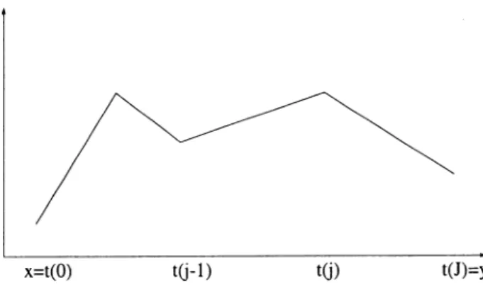
(6) 138. BERNHARD. KAWOHL. AND. CHRISTOPH. SCHWAB. We can now turn to the proof of Theorem 2.1. Proof of Theorem 2.1. To prove statement (i), we consider F( 0) and CN ( l) separately. For the smoothness of F(a), we use (2.2). Let & E [0, Ml3 denote the vector of nodal variables of u E SN on Tk. Then Vu ]*k = A& where Ak E R2x3 is a certain matrix depending only on the nodes of Tk. Hence, by (1.8), f(Vu 1~~) = f(A&) E CkyA([O, M13). Now, according to (2.2), F(u) is a finite linear combination of such terms and therefore F() E Cky*([O, MIN). Consider now CN(-). Again it suffices to verify that each term in the finite sum (2.6) is, as a function of the nodal values & and u’e, in C LsJ~s-LsJ([0 M14). Since two of the six nodal values are identical due to the continuity of u across ektl we denote the vector of the four ‘essential’ nodal values of u on Tk U Te by u’k&Then a typical term in the sum(2.6) is 1[&&e]- (swhere &[ is a certain matrix dependingonly on the nodepositions of Tk and Tt. For this term, however, the smoothnessis immediate. To prove assertion(ii), we first showthat ur exists. To this end observe that by (i) F(v) and CN(u) are continuous functions of the nodal values U(Pi) of IJ E Sg on the closedand boundedset [0, M] N. Hence, for every E > 0 and every N, there exists a minimizer uf of F + s-‘CN on Sg by the WeierstrassTheorem. To show (2. lo), for a given triangulation TN choosex, y E U,“=‘r’ 5 and connect them by a straight line Xy c Q (here the convexity of 52 is used).The assertionis only nontrivial if Xy is not contained in one element Tj which we assumefrom now on. As a function of the arclength t along Xy, u: is a piecewiselinear function u(t) like the one depicted in Fig. 1 with breakpointsat the transversalintersectionstj, j = 1, .... J - 1 of Xy with certain interelement edgesej-t,j acrosswhich Vu: may jump. The (weak) derivative v’(t) is piecewiseconstant, i.e.. 4(. = vi Q-1. j. Jj). =l. J. 9 .**9. and v@J>. =. v;(tJ. -. Q-1). +. eL-1). =. v;(tJ. -. tJ-1). +. v;-#J-l. -. b-2). +. m-2). .. . J =. U(t0). +. >:. uJ(tj. -. tj-1).. +. z($. j=l. Hence J U(tJ). -. u(t()). =. v;(tJ. -. to). -. vi-,)(tJ. -. tj-1).. j=2. This yields the inequality u(tJ>. -. v(tO). <. v; @J -to). +. x[v>-l. j=2. The estimate (2.10) will be derived from (2.14).. -. u;]-(tJ. -tj-1).. (2.14).

(7) CONVERGENT. x=t(O). FINITE. Q-1). t(J)=Y. t(i). 1. The function. FIG.. 139. ELEMENTS. u (t ) along the line Xy.. Assume first that Xy doesnot intersect any node of 7~. Then no interelement edge is completely contained in Xy and each of the straight line segmentsin the intervals @j-r, tj) in Fig. 1 is contained in some triangle, Tj say, of TN. As uf is piecewise linear, Vu: is constant on Tj and we denote its value by Vu:(j), j = 1, ..., J. Moreover, vi = Z&Q&j) wherezXy = (y-x)/ Iy - xl. Denotingxo = x, xj = y andxj = ~fkj-r,j, =l J 1, we get from (2.14) that j 9 l ‘*Y. u,N(y). -. u:( x ). <. V&x). l. (Y. -. xl. J. +x. [(Vuf(j. -. 1). -. Vu,N(,jl). l. &yl-. IY. -. xi-1. 1. l. j=2. Since the jump of Vu: along the interelement edgeej-r,j is zero, an oblique jump can be estimatedby the jump of Vu! in the direction of the exterior unit normal Zj-r,j to Tj-1 pointing into Tj. This yields the bound. l&y). -. u,N(x). <. vu;(x). l. (Y. -a. J +. >:. [(Vu,N(j. -. 1). -. Vu,N(j>). -. 1) -. l. zj-l,j]-. IY -Xi-l. (2.15). j. j=2. <. Vu,N(x). +. l. (. kiL( j=2. (Y. -. J. x). Vu,N(j. 1/s*. Vu,N(jl)l zj-1,j l-ls)l’s (E IY- Xi-1 1” j=2 1. by Holder’s inequality in Rj-’ with s* = s/(s - 1). Since the triangulations 7~ are quasiuniform, there exists a constantc independentof N suchthat J < c Ix - y I/ h. Therefore J >:I j=2. Y - Xi-1 IS*< J 1~-. XI'*. < C (diamQ) Ix - ylS* /h..

(8) 140. BERNHARD. KAWOHL. AND. CHRISTOPH. SCHWAB. Inserting this into (2.15) results in l&y). -. u,N(x). <. Vu,N(x). l. (Y. -4. +c (diam n)“‘*. h-‘I”*. (CN(ur)). I” Ix - ~1. (2.16). with a constant c independent of E and N. Now f(p) > 0 and u = M E CM imply 1. 0 < F(u,N>+ -CN(U,N>< F(M) = f (0) IQ1 & from where we get. 0 < CN(U,N)< f(O) WI &*. (2.17). Inserting this into (2.16), we obtain U,N(Y) - u:(x). < Vu:(x). . (y - x) + c (diamQ)‘/“* (f(0) IsZlg)‘lS Ix - yl /z-‘/~*. which is (2.10). In the case that Xy contains a node pi or an entire edge, we argue by continuity: (2.10) hasbeen proved for almostall x, y E Q and u$’ is continuous, therefore (2.10) is true everywhere. To prove (iii), we note that (2.10) and (2.11) imply ';N)(Y>. -. N 'e(N). x,yEG. (X)-VU~N)(X)~(y-~)~~(E(N))Bl~-yl,. (2.18). where/? = (l-a(sl))/s > 0. Functions in CM satisfy (2.18) with c = 0 and exhibit, by Proposition 1.1, good compactnessproperties which allow us to apply the Direct Method in the Calculus of Variations (see,e.g., Dacorogna(1989)) to (1.6). We shall extend this to functions satisfying (2.18). We proceedin several steps.. StepI: We prove that (u:N) )N contains a subsequencewhich convergesin Wlf;,$'(12),1 < p<oo,toalimituEC~. For a given x E 52 choosein (2.18) the point y E X2 in sucha way that the vector y - x points in the direction -VU~N) (x) (i.e. into a direction of steepestdescentof u&)). Then N I. vu;,)(x). ( <. -. ue’N’(;) X-. u$V)(Y) yI. + c (ww~. M < dist(x, X2) + c (E(N))~ . (2.19). Therefore the sequence{u&) )N is uniformly boundedin Wlf,cm(i2). Since (u&) }N is uniformly Lipschitz continuous on every $2’ CC 52, there exists a subsequence(again denoted (u&,] }N) which convergesweakly in every W*J’(Q’), 1 <. p < 00 and uniformly on 52’ to a limit u E W&/($2), 1 < p < 00. Let US show that VU$N) convergespointwise almost everywhere in $2’ to Vu. To this end, we adapt an idea of Marcellini (1990) (seealso Rockafellar (1970)). Let ei denotethe unit vector in the direction of the ith coordinate. Each u& is differentiable a.e. in 52’ and so is u. Let x be a point in which each u&) and also u are differentiable (the set of points.

(9) CONVERGENT. FINITE. 141. ELEMENTS. where this is not the case is a countable union of measure zero sets and hence has measure zero). According to (2.10) we have for sufficiently small S > 0 and any E > 0. uf(x+ 6ei)- U,N(X). <. SDiu,“(x). +. cE'~. <U:(X)-Uu,N(X. 2CE'S.. -6ei)+. We select E = E( N ), send N to infinity and obtain, upon dividing by S > 0, U(X. +6ei). -U(X) 6. < lim. SUP. -. Diu$Nj. <. c. U(X)-. J9-r(E(N))B U(X. < 1bmi.f Diu$,,). -6ei). + c lim (E(N))~.. s. N+CXl. N-+03. Next we send S to zero and note that the upper and lower bounds for DiU$N) converge to Di u . Therefore lim Vu$&) = Vu(x) a.e. x E a’. N+CQ. By the Lebesgue dominated convergence theorem, the sequence {u$$ converges to u strongly in W’yP (Q’), 1 < p < 00, for any a’ CC Q. Since a’ wasan arbitrary subsetof + Vu pointwise a.e. in 52.Therefore we may alsousethe Lebesguedominated a, “;N) convergencetheorem to conclude that. F(u;N)> + F(u). (2.20). holds. We claim that u E CM. To prove it, we observethat by (2.18) the limit u(x) must satisfy (2.5). This implies that u E CM. Step 2: Let uN be a minimizer of F over CM n SN. We show that (a subsequence of) (u N}N. convergesto a solution Gof (1.6). We first show that for every N a minimizer uN of F over CM n SN exists. To this end, we fix TN and let E tend to zero: Since the sequence{u~JE,~ is determined by the nodal values (ur(Pl), .... uf (PN)) E [0, MIN on the fixed triangulation TN, the theorem of Heine and Bore1 ensuresthat a subsequence((u,“:(PI), ..., u$ (PN)))$>() convergesto some(al, .... aN> E [0, MIN. Denote by uN E SE the piecewiselinear function with nodal values UN(Pi) = ai. Then, by construction,. E’ -UN11 wl*yL?) +O II UN. as. E’ + 0.. (2.21). Moreover, since both u,“: and uN are piecewiselinear with function values in [0, M] there exists a constant A (N, M), independentof E’, suchthat. lp4llLm(R)’ IPUNIL(Q)GA(N,w (with the derivatives taken in the senseof distributions). Due to (2.21) and the uniform continuity of f(p) on [0, A]* it follows that F(uz) + F(uN). as. Et -+ 0.. (2.22).

(10) 142. BERNHARD. KAWOHL. AND. CHRISTOPH. SCHWAB. Further, due to (2.17) we have 0 < CN(uF) < f(0) lJ2l c’ which implies that CN(uN) Therefore u N E SN n CM. Moreover, we claim that F(uN). =. min. F(u).. = 0. (2.23). l&PM*. To prove it we observe that the inclusion SN n CM c SL implies F(u;). 1 + -CN(u;> E’. < F(u$). 1 < F(v) + 7CN (v) = F(v). for every 8/ > 0 and every v E SN n CM since CN (v) = 0. We let E’ tend to zero and use (2.22) to obtain (2.23). By Proposition 1.1, (a subsequence of) (u N, converges strongly in W,::(D), 1< p < 00, to a limit ii E CM. We claim that ii is a minimizer of F on CM. To prove this, let v E CM be given. Then, by Lemma 2.1, v can be approximated by a sequence vN E CM n SN in W ‘VP(a’) for every 52’ cc a, 1 < p < 00. Now pick Q’ CC Q such that the set Q\a has measure less than ~1, say. Then pick N sufficiently large so that IIv - vN IIwl.p(~l) < ~2. Since the density f(p) is uniformly bounded we have. F(v) 2s Q’. fWW. -El Ilfllp 9. (2.24). and since f is uniformly continuous on bounded sets, due to Egorov’s theorem. s. f won. -. Oh). x2’. a s sz’. f wvNm. -. Wl>. -. W&2). with O(Q) uniform in N. Combining this with (2.24) and using the minimizing property (2.23) of uN gives F(v). > F(vN). - O(Q) - O(E~) 2 F(uN). - O(Q) - O(Q).. (2.25). By the same arguments, choosing 52’ as above and N such that 11ii - uN 11wI,p(sz,I < e2, we obtain F(uN). > F(ii) - O(Q) - O(e2).. (2.26). Now (2.25) and (2.26) lead to F(v). 2 F(ii) - O(e). for any v E CM, & > 0,. that is G minimizes F on CM. Step 3: Finally we show that the limit u of (a subsequence of) the sequence u&) of the FE solutions obtained in Step 1 satisfies F(u) = F(i), i.e. u is a minimizer of F on CM. To this end, observe that for the sequence {u N } from Step 2 we have F(uN). = F(uN). 1 + -CN(uN) W). 2 F(u&)). 1 + -CN(u&$ WV. 2 F(U$&-.

(11) 143. CONVERGENTFINITEELEMENTS. As shown in Step 2, after passingto a subsequenceif necessary,the left-hand side convergesto F(c). By (2.20) and (2.17), the right-hand sideconvergesto F(u) and therefore we have shown cl F(i) > F(u). Since ii E CM was a minimizer, so is U. This completesthe proof. REMARK. 2.1. The boundednessof the density f was used only in Step 2 of the above. 2.2. If the minimizer u is unique, the whole sequenceU& convergesto u.. proof. REMARK. 2.3 Step 2 of the proof showsin particular that conforming (i.e. concave) FEapproximations uN E CMMN exist and, possibly after passingto a subsequence,converge to a minimizer u. REMARK. 3. Minimization of the discretized problems In the previous sectionswe showedconvergence results for sequencesof finite element solutions u,” and uN of (1.6). These solutions, however, must be computed by solving a finite dimensionalminimization problem of the form min G(u) ~OI~lN. (3*1). where u = (ui, .... UN) E RN denotes now the vector of nodal values of the finite element solution and G(e) is the objective function correspondingto (2.7). Our purposein the presentsectionis to introduce a classof algorithms suitablefor the finite dimensionalminimization and to presentcorrespondingconvergenceresultsfrom Bertsekas(1982) which are valid in our setting. Throughout, we assumethat G is at leastin Cl” ([0, MIN), i.e. that. W(x) - VG(y)l < L Ix -. YI. Vx, y E [0, MIN.. WI. According to Theorem 2.1 this is the caseifs > 2 and if f(p) E C’T’ (R2). The discrete minimization (3.1) can be performed with a classof projected descentalgorithms which we now describe.To this end, we denote. 1x#1 := max(O, min(x, M)),. x E JR,. and we write for u E RN. cU1# := ([ul]# , [@]#, .... [u&e The first-order necessaryconditions for a vector U to be a local minimum of (3.1) are &G(G) 2 0. if Ui = 0,. &G(i). < 0. if Ui = M,. &G(i). = 0. else.. (33. Here and in what foll .ows,ai denotesthe partial derivative with respectto the ith coordinate. The minimization algorithms we considerare of the form (Bertsekas(1982)) u(k+l). = dk)(@k). 9. dk)(a). =. [dk). + ap(“q#,. a > 0. (3 04).

(12) BERNHARDKAWOHLANDCHRISTOPHSCHWAB. 144. where @kis a stepsizeand pCk)is a descentdirection, suchasfor example P(k) = -Dck’VG(u(k)) .. 65). Here Dck) is a sequenceof positive definite, symmetric scalingmatricesstill at our disposal. According to Bertsekas(1982), the sequenceof matrices Dck) and the stepsizes@kwill be chosen as follows. Let a small number S > 0 and parametersp E (0, 1), 0 E (0, i) be given. Define - VG(U(~))]#~ ,. wk =. 8k = min(S, wk).. Then the index set r,# of active constraints at iteration k is I#k. <. 6k 9. aiG(uck’). >. 0 Of M. -. 8k <. Uck) i. <. M,. aiG(uck’). <. 0. The scaling matrices DCk)are assumedsymmetric, positive definite and diagonal with respect to Ik#’i.e. Dtk) = 0 ij. Vi, j E Ik#,i # j.. The stepsizesak in (3.4) are given by ak = pm”. (W. where ?nkis the first nonnegative integer suchthat G (dk’) - G(dkQm)). 2 o pm x aiG(U(k))p!k) + x I iftIt id:. &G(uCk))[uy) - u~‘(/Ym)] . I W). For the minimization algorithm thus defined, we have the following convergence result (Bertsekas(1982)). 3.1 Assumethat the matrices DCk)are diagonal with respect to the index sets1: and uniformly positive definite, i.e. there exist hi > 0 independentof k such that PROPOSITION. A1 lx12 < xTDCk)x < A21x12. VxdRN,. k=O,l,.... and that (3.2) holds. Then every limit point of a sequence(Uck’)generatedby the iteration (3.4~(3.8) is a critical point of (3.1). 3.1 A basic special case is the method of steepestdescent with projection which is obtained by selecting in (3.4) a!k = a! > 0 sufficiently small and DCk)in (3.5) to be the unit matrix. This method convergeslinearly. REMARK. It turns out that under someadditional assumptionson G and the minimum U the algorithm (3.4), (3.5) displays local superlinearconvergence.To describe theseassumptions, define for u E [0, M]* the set B(u) of indicesof binding constraints at u, i.e. B(U) = {i I ui = 0 or ui = M).. (3.9). Consider now an isolated local minimum ti of G for which there exists 8 > 0 such that.

(13) 145. CONVERGENTFINITEELEMENTS. G E C* in the open ball of radius 8 with centre at u’ and there exist further 0 < Ai < A2 suchthat for all x E lEJLN with xi = 0 for i E B(u’). A1 1x1* < xTH[G(u)]x. < A2 1x1* V lu - Ul < 8. (3.10). where H[ G (u)] denotesthe Hessianmatrix of secondderivatives of G () at U. In addition, we require (3.3). The following result from Bertsekas(1982) showsan important property of the descentalgorithm, namely that the set B(ii) is identified afterfinitely many steps,i.e. I#k = B(u(~)) = B(C) PROPOSITION. 3.2. Vk 2 k.. (3.11). Let U be a local minimum of G satisfying (3.10) and (3.3) and assume. that 0 c 11 < Df’. i E Zf,. k = 0, 1, ..... Then, if u(O)is sufficiently closeto U, the sequenceutk) generatedby (3.4)-(3.8) converges to U and (3.11) holds. This implies in particular that for k 2 k in (3.11) the descentalgorithm with projection reducesto an unconstrainedone operating on the free indices ( 1, ..., N}\ B(C). By a suitable selection of the matrices DCkJ,e.g. portions of the inverse Hessianof G at uck)or quasiNewton update approximations of it, locally quadratic resp. superlinearconvergencerates are achieveableunder standardassumptions,such as G E C3([0, MIN). By Theorem 2.1, this holds for densitiesf(p) E C3(W*) and s > 3. 4. Numerical results In the presentsection we report numerical resultsobtained from a finite elementdiscretization of (1.6) with F(u) = R(u) and the algorithm (3.4), (3.5). We solved (1.6) on the domain D = (-1, l)* and reduced the finite element calculation to one quadrant (0, l)* using the symmetry conditions u(xl,x*). =. U(Xl,. -x2). =. u(-x1,x*). =. u(--xl,. -x2).. Wl). 4.1 Obviously the domain (- 1, l)* and the functional are invariant under the variable changes(4.1). It is an open question whether this implies the correspondingsymmetry for the minimizers, i.e. the existence of asymmetric minimisersfor symmetric domainscannot be ruled out at this point. REMARK. All statementswhich follow in this sectionrefer to the domain (0, l)*. We used a uniform meshconsistingof triangles obtained from a subdivision on (0, l)* into N* quadrilaterals and bisection of each quadrilateral along the diagonal parallel to Xl = x2. We started the iterations from the initial, concave profile w. 9 x2). =M(12p).. VW. The sequenceof scaling matrices Dtk) in (3.5) was selectedto be the unit matrix and, according to Remark 3.1, the stepsizesak were selectedconstant. The value of E which.

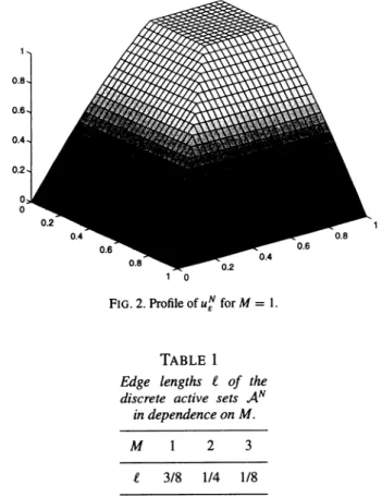
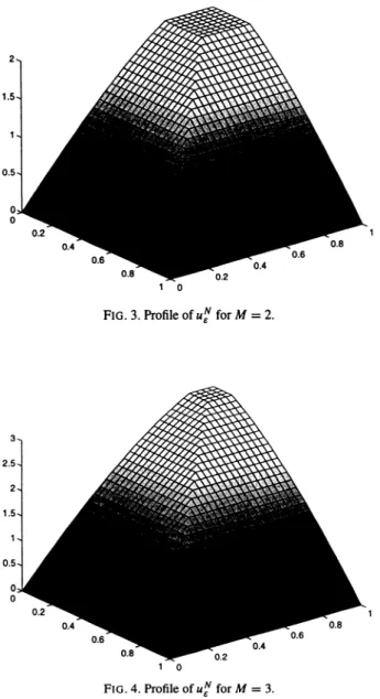
(14) 146. BERNHARD. KAWOHL. AND. CHRISTOPH. SCHWAB. 0.8 0.6. FIG. 2. Profile of uf for M = 1.. TABLE. 1. Edge lengths kf of the discrete active sets AN in dependence on M. A4. 1. 2. 3. e. 318. l/4. l/8. was important for the convergenceof the scheme,was actually chosenfairly large, in our case we selected E = 20. This choice of E was sufficient to keep the value of C(uf) below 0.01 throughout the descentiterations. Selecting a much smallervalue of E increases the stiffness of the discrete problem substantially and reducesthe feasible stepsizes.We performed 10000stepsof (3.4) (with parameterS = 0.01) which, due to the explicit nature of the algorithm, can be executed quite efficiently. In this fashion we obtained profiles u:(x) for M = 1,2,3 and a meshwidth of h = l/32 (correspondingto N = 1024degrees of freedom) correspondingto nodal values of (ih, jh), 0 < i, j < 32. Figures 2, 3 and 4 depict the profiles thus obtained for A4 = 1,2,3, respectively. The approximate minimizers found in this fashion exhibit the following structure. They all have a discrete active set dN which is a squarecentred at the origin and with the edge lengths listed in Table 1. It appearsthat the edge length is decreasingas M increases,i.e. as the profile gets more slender.As is visible in Fig. 3, the profile is nondifferentiable at i3dN. However, unlike the unsmoothnessencountered for elliptic problems with constraints (as, for example, the obstacle problem), here the gradient of u (rather than the secondderivatives) has a jump at iId. Moreover, the profiles exhibit a smoothly curved edgeemanatingfrom each vertex of dN and connecting the vertex of dN with the nearest.

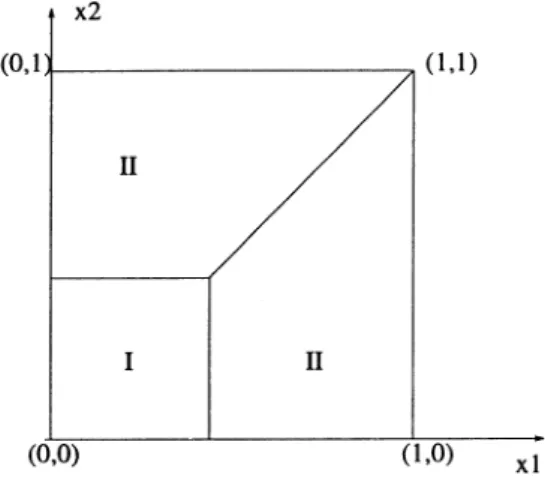
(15) CONVERGENT. FINITE. 0.8-70.2. ELEMENTS. 147. "-1. 0. FIG. 3. Profile of uf for A4 = 2.. FIG. 4. Profile of uf for M = 3.. comer of (- 1, 1)2. In Fig. 5 we sketch schematically the domains where U: appears to be smooth. The set dN corresponds to I. For M = 2 and M = 3, the profile in the subregions labelled II appears to be a developable surface parallel to the edge of dN. In Table 2, we show the nodal function values for (uf)ij for M = 2 and j = 9, i.e. along the first vertical mesh line not contained in dN. We see that the slope of the gradient in the region II near 3dN is roughly (2 1l969)/ h = 0.03 1 x 32 = 0.992 which is evidence for the conjecture that IVu 1 = 1 along the straight segments of ad. In fact, as remarked on page 75 of Buttazzo et al (1995), or.

(16) BERNHARDKAWOHLANDCHRISTOPHSCHWAB. 148. FIG. 5. Scheme of the subdomains I and I I.. TABLE 2 Nodal coordinates (u:)ij for M = 2 and j = 9.. i. cue1 N. i.9. 0. 4. 8. 12. 16. 20. 24. 28. 32. 1.969. 1.969. 1.969. 1984. 1.69. 152. 1.33. HO. 0*77. TABLE 3 Numericalvaluesfor the relative resistance R(uf )/ IQ I.. M. 1. 2. R(u,N)/ IQ1 0.372 O-172. 3 0086. page478 of Whiteside (1974), Newton already knew that an optimal (rotational) body will have a blunt front end d with the slope of u jumping from zero to one on ad. Nobody seemsto know, though, how Newton arrived at this insight, seeWhiteside (1974). For nonrotational bodies(or nonradial minimizers u) it is natural to conjecture the samebehaviour. This was discussedand partly proved in Buttazzo et al (1995), p 87. We close with a listing of the numerical values for the relative resistance,defined by I?@:)/ IInl, for Q = (-1, 1)2 (seeTable 3)..

(17) CONVERGENT. 5. Concluding. FINITE. ELEMENTS. 149. remarks. The restriction to plane polygons Q is not essential for the convergence result Theorem 2.1. If Sz is a convex polyhedron in Iw”, it > 2, the proof of Theorem 2.1 still applies verbatim. Although we considered explicitly only the case of polygonal domains and f (x, u , p) = f(p) in the present paper, our proofs can be modified in the case of curvilinear boundaries and general densities f, provided f is a sufficiently smooth function of its arguments. The convergence analysis of higher-order elements for (1.6) can be based on the ideas in the present paper, but several new technical issues, such as numerical integration and proper enforcement of the constraint 0 < u(x) < M must still be resolved. Acknowledgements The research of BK was supported in part by the German Research Foundation (DFG) via the ‘Sonderforschungsbereich No 359: Reaktive Stromungen, Diffusion & Transport’; that of CS by IBM Germany with the resources of the IBM Scientific Centre, Heidelberg, where part of the paper was written while CS was a visiting researcher there. CS also gratefully acknowledges partial support from the AFOSR under grant No F49620-J-0100. REFERENCES ADAMS, R. BERTSEKAS,. A. 1978 Sobolev Spaces. New York: Academic. D, 1982 Projected Newton methods for optimization problems with simple constraints. SIAM J. Control Optimiz. 20,221-246. BUTTAZZO, G., FERONE, V., & KAWOHL, B. 1995 Minimum problems over sets of concave functions and related questions. Math. Nachrichten 173,71-89. CIARLET, P. G. 1978 The Finite Element Methodfor Elliptic Problems. Amsterdam: North-Holland. DACOROGNA, B. 1989 Direct Methods in the Calculus of Variations (Springer Applied Mathematical Sciences 78). Berlin: Springer. FEISTAUER, M., & NECAS, J. 1985 On the solvability of transonic potential flow problems. 2. Anal. Anwendungen 4,305-329. LIONS, P. L. 198 1 Generaked Solutions of Hamilton-Jacobi Equations (Research Notes in Mathematics 69). Boston: Pitman. MARCELLINI, P. 1990 Nonconvex integrals in the calculus of variations. Proc. of “Methods of Nonconvex Analysis ” (Varenna, 1989) (Springer Lecture Notes in Mathematics 1446) Heidelberg: Springer (A. Cellina, ed). pp 16-57. MIELE, A. 1965 Theory of Optimum Aerodynamic Shapes. New York: Academic. NEWTON, I. 1686 Philosophiae Naturalis Principia Mathematics. ROCKAFELLAR, R. T. 1970 Convex Analysis (Princeton Mathematics Series vol. 28). Princeton, NJ: Princeton University Press. WHITESIDE, D. T. 1974 The Mathematical Papers of Isaac Newton vol. VI. London: Cambridge University Press..

(18)