An Experimental procedure for deriving Z-transfer function coefficients of the building envelope

Publisher’s version / Version de l'éditeur:

ASHRAE Transactions, 97, 2, pp. 90-98, 1991

READ THESE TERMS AND CONDITIONS CAREFULLY BEFORE USING THIS WEBSITE.

https://nrc-publications.canada.ca/eng/copyright

Vous avez des questions? Nous pouvons vous aider. Pour communiquer directement avec un auteur, consultez la

première page de la revue dans laquelle son article a été publié afin de trouver ses coordonnées. Si vous n’arrivez pas à les repérer, communiquez avec nous à PublicationsArchive-ArchivesPublications@nrc-cnrc.gc.ca.

Questions? Contact the NRC Publications Archive team at

PublicationsArchive-ArchivesPublications@nrc-cnrc.gc.ca. If you wish to email the authors directly, please see the first page of the publication for their contact information.

NRC Publications Archive

Archives des publications du CNRC

This publication could be one of several versions: author’s original, accepted manuscript or the publisher’s version. / La version de cette publication peut être l’une des suivantes : la version prépublication de l’auteur, la version acceptée du manuscrit ou la version de l’éditeur.

Access and use of this website and the material on it are subject to the Terms and Conditions set forth at

An Experimental procedure for deriving Z-transfer function coefficients

of the building envelope

Haghighat, F.; Sander, D. M.; Liang, H.

https://publications-cnrc.canada.ca/fra/droits

L’accès à ce site Web et l’utilisation de son contenu sont assujettis aux conditions présentées dans le site LISEZ CES CONDITIONS ATTENTIVEMENT AVANT D’UTILISER CE SITE WEB.

NRC Publications Record / Notice d'Archives des publications de CNRC:

https://nrc-publications.canada.ca/eng/view/object/?id=94c544d4-0446-4123-8bbc-938fa6f983e4 https://publications-cnrc.canada.ca/fra/voir/objet/?id=94c544d4-0446-4123-8bbc-938fa6f983e4

An Experimental procedure for

deriving Z-transfer function

coefficients of the building

envelope

Haghighat, F.; Sander, D.M.; Liang, H.

NRCC-35511

A version of this document is published in:

ASHRAE Transactions, 97, (2), ASHRAE Annual Meeting

(Indianapolis, Indiana, USA, June-22-91), pp. 90-98, 91

The material in this document is covered by the provisions of the Copyright Act, by Canadian laws, policies, regulations and international agreements. Such provisions serve to identify the information source and, in specific instances, to prohibit reproduction of materials without written permission. For more information visit http://laws.justice.gc.ca/en/showtdm/cs/C-42

Les renseignements dans ce document sont protégés par la Loi sur le droit d’auteur, par les lois, les politiques et les règlements du Canada et des accords internationaux. Ces dispositions permettent d’identifier la source de l’information et, dans certains cas, d’interdire la copie de documents sans permission écrite. Pour obtenir de plus amples renseignements : http://lois.justice.gc.ca/fr/showtdm/cs/C-42

4

1

AN EXPERIMENTAL PROCEDURE

FOR DERIVING Z-TRANSFER FUNCTION

COEFFICIENTS OF A BUILDING ENVELOPE

F. Haghighat, Ph.D.

Member ASHRAE

D.M. Sander, P.E.

Member ASHRAE

H. Liang

ABSTRACT

The z·transfer function method is used in calculations for HV AC system design and building energy consumption. Calculation methods to determine the z-transfer function coqflcients, which characterize the dynamic thermal peiformance of building components, do exist, but these depend on a number of assumptions and one must sup-plement them with experimentally derived coefficients.

This paper discusses the use of system identification techniques to derive the dynamic thermal response of building components using binary multi-frequency sequence (BMFS) signals. BMFS were implemented to determine the frequency response function of the system at multi-frequen-cies. The z-transfer function coefficients are obtained by applying multi-Unearregression techniques to the frequency response.

ｔｨｾ＠ z-transfer function coqflcients also were obtained using /ilast-squares regression in the time domain.

INTRODUCTION

The ASHRAE Handbook-1977 Fundamentals

(ASH-RAE 1977) describes the

use

of the z-transfer function technique for predicting the rate of heat flow through exterior walls. In this technique, the z-transform of the heat flow at the inside surface of the wall,

Q

_1, is related to the z-transform of the room air temperature, T1, and the

z-transform of the sol-air temperature at the outside surface,

T

2, by

(1)

where 1/B(z) is the transfer function that relates the heat flow at the inside surface to the temperature at the outside surface and D(z)/B(z) is the z-transfer function that relates the heat flow at the inside surface to the room air tempera-ture variation. These transfer functions characterize the dynamic behavior of the wall. They depend on the physical propP.rties and thickness of the material. The z-transfer functions, 1/B(z) and D(z)/B(z)

1 can be written as the ratio

of two finite polynomials in

z- :

1

--·

B(z) (2) and D(z) B(z) -1 -2 -1 = ｟｣ＮＡ ＰｾＫ｟｣ＮＮＮＡ ＱｾｺＮＮＮＬＮＮ｟Ｋ｟｣ＮＮＺ Ｒ｟ｺＭＺＺＭ｟Ｋ｟Ｎ｟＠ •• _+_c_,1:..z_ 1 b ₊

_.z

-1 + b 2.% -2 _{+ ••• +} b -·

.z

(3)

where a, b, and care transfer function coefficients, and z-•

is an operator indicating a delay of ml., where .:l. is the time interval

used

for simulation calculations. For most air-conditioning load calculations, the room air temperature can be assumed to be constant and only the

liB

transfer function is required. The z-transfer function coefficients for 179 different construction types are tabulated in ASHRAE (1977). These coefficients were calcnlated by a computer program using the known thermal properties of materials (Mitalas and Arseneau! 1972). Use of these coefficients implies the assumption that the walls and roofs consist of layers of homogeneous materials and that heat flow is one-. dimensionalone-. In practice, however, the properties of the

materials are often unknown, and actual walls contain heat bridges, such as framing studs, fasteners, anchors, etc., and may be composed of nonllomogeneous materials. Further-more, the properties of the materials in a wall may be unknown. Therefore, there is a recognized need for meth-ods to derive transfer function coefficients of building envelope components from experimental data.

Pedersen and Mouen (1973), as part of an ASHRAE research project, attempted to derive the thermal response factors of a wall from measured data. They concluded that the direct

procedure

for determining thermal response factors was Impractical

because

of the extreme sensitivity to experimental error.

Crawford and Woods (1985) used least-squares techni-ques to fit parameters to a chosen transfer function model in the time domain. Fang and Grot (1985) derived thermal resistance values of building envelopea from field data. Barakat (1987) experimentally determined the cooling load z-transfer function coefficients and the room air transfer function coefficients for houses. Haghighat et al. (1988) developed a technique to derive the cooling load z-transfer function coefficients from experimental data using linear regression techniques. Seem and Hancock (1985) presented a technique for characterizing the dynamic performance of a thermal storage wall based on the data obtained from a series of temperature and heat flux measurements. The coefficients of a transfer function model were estimated directly from data using linear least-squares regression.

Fariborz Haghlghat is a Research Assistant Professor and Hong Liang is a Research Assistant at the Centre for Building Studies,

Concordia University, Montreal, Quebec, Canada. Daniel M. Sander is a Senior Researcher at the National_ Research Council Canada,

Ottawa, Ontario.

Stephenson et al. (1990) developed an experimental procedure to derive the transfer functions of walls. Their procedure involved the following steps: starting from the time constants expression of the transfer function in the

s-domain, they determined the

time

constants and the as-sociated residues from measurements of tests using a ramp input signal. Then, using the equivalence between the time constants expression and the ratio of polynomials expression of the z-transfer function, they found the z-transfer function coefficients in the denominstor of the expression. Next, they determined the frequency

response

from tests using sinusoidal input signals and matched this frequency response to the

response

of the z-transfer function at those specific frequencies in order to determine the coefficients in the numerator of the z-transfer function.

Haghighat and Sander (1987) used system identification techniques to determine the dynamic response of a single-layer sample. In their study, a wall was considered as an unknown system with an input (outside

surface

temperature variation) and an output (the hest flux on the inside surface of the wall) related by a transfer function. The experimental procedure used a binary multi-frequency sequence signal (BMFS) as the input driving function.

The

coefficients of the z-transfer function 1/B(z) were obtained for the single-layer sample using both frequency response analysis and lesst-squares regression in the time domain.

To investigate the thermal performance of walls due to both indoor and outdoor condition variation, Haghighat et al. (1991) used the frequency response analysis method mentioned above to determine the other transfer functions in the pipes' transmission matrix.

The

dynamic frequency response agrees fairly well with that obtained from analysis. This paper describes the application of the experimental procedure for derivation of z-transfer function coefficients for 1/B(z) to both a single-layer and a multi-layer sample. SYSTEM IDENTIFICATION METHODOLOGY

Numerous techniques for experimentally determining a dynamic model for a process from input/output messure-ments have been reviewed by Astrom and Eykhoff (1970) and Bekey (1970). The formulation of the identification problem as proposed by Bekey consists of (a) selection of the form of the model and determination of the parameters, (b) choice of an input signal, and (c) selection of a criterion for determining the "goodness" of the model and a method for adjusting the model parameters to optimal values based on this criterion.

In this study, the form of the model was predetermined to be the z-transfer function recommended by ASHRAE. In

the z-domain, this function is H(z) • Q(z) T{z) -1 -2 -II ｾｾｯＫ｡ _Ｑ ｺ＠

+a,z + ... +a.z

=

ＭＱｾ｢ｾＭＮＷＱＭＭ｢ｾＭｾＲｾＭＭＭＭ｢ｾＭＭＭｍ＠ + 1% + 2% _{+ .•• +}

_.z

and in the time domain it can be written as

II Q(t) =

:E

a,

T(t -

i4)

1=0 lit

- :E

b

₁

Q(r-

i4)

i= 1 (4) (5) 91 wfuJre Q(t)

=

output at time t, :Itt)

=

input at time t, and

4 = time interval used for simulation.

The number of terms,

n

or

m,

is less than seven for all wall constructions tabulated in ASHRAE (1977) and is usually less than four.

One

of the main requirements of an input signal for system identification is that it should be sufficiently rich in components of distinct frequencies to excite all important modes of the system.

The

input signal chosen was a binary multi-frequency sequence (BMFS}, which contains sig-nificant signal amplitudes at several different frequencies. Binary signals have the advantage that ouly simple switch-ing control elements

are

needed to generate the signal.

In this study, the input/output signals were analyzed using two methods.

One

is the frequency analysis proce-dure, which consists of transforming experimental data to the frequency domain using

the

Fast Fourier Transform (FFT) and determining the frequency response of the transfer function, then applying multi-linear regression techniques to fit z-transfer function coefficients to the frequency response. The second method is to determine the z-transfer function coefficients using conventional multi-linear regression in the time domain.

In the frequency analysis procedure, the criterion is to

minimize

the difference between the frequency response of the model and the messured response of the sample. The messured frequency response function was determined by performing a discrete Fast Fourier Transform on input and output signals and then taking the ratio of output to input at each frequency,

f,

at which the input signal

had

a

com-ｰｾ＾ｮ･ｮｴ＠ of significant amplitude:

where

H(/) • Q(/)

T(J) (6)

Q(j)

=

FFT of output, Q(t), at frequency

f,

and

7Yj) = FFT of input, Jtt), at frequency

f.

The frequency

response

function can be conveniently depicted on a Bode plot, which is a graph showing the amplitude and phase of H vs. frequency.

The common criterion for choosing the optimal values of parameters is to

minimize

the square of the error, where error is the difference between the model and process output. Since the frequency response, H, is complex, the squared error for the frequency response function is defined as

wfuJre

ｾＰＰ＠

₁₀₀

H''""

H'Iw

= real

part

of messured response at frequency

f,

=

imaginary

part

of measured response at

fre-quency/,

= real part of model response at frequency

f,

and

= imaginary part of model response at frequency

f.

The procedure for fitting coefficients to the ｾｯ､･Ａ＠ of Equation 4 is shown in Appendix A. Two equatiOns, one for the real part and one for the imaginary part, can be written for the frequency response of the model at every

Heater H1

Heater

Tl

Figure

1

Schematic of test apparaJus

frequency for which the measured response is available. An additional equation equates the steady-state response to the

measured U-value. For N frequencies, this results in 2N

+

1 equations, which are solved for the z-transfer function coefficients uaing least-squares multiple linear regression.

The time domain regression analysis consists of applying the measured input/output values to Equation

5

and obtaining the coefficients uaing multiple linear regres-sion.

TEST

ｾｒｏｃｅｄｕｒｅ＠

FOR DERIVATION OF TRANSFER FUNCTION 1/8

From Equation

1,

the definitionoftransfer function

liB

is

where

T = 1 j - T2,

7j

=

room air temperature, and

T₂

=

sol-air temperature at outside surface.

(8)

To derive transfer function

liB,

the experimental setup must satisfy the following conditions: (a) maintain the temperature T1, constant; (b) vary the temperature T2; and

(c) measure the heat tlux, Q,.

The· experiment was

set

up as shown in Figure 1 in order to meet these requirements. Three heaters were used: heater H₁

was

controlled to maintain temperature 7j constant; heaters

H.,.

and

H;,.

were

controlled by the input signal to produce a varyiilg temperature

T

2• Two cold

plates, through which liquid at constant temperature was circulated, served as a sink for the heat from the heaters. Using this symmetrical configuration, the heat tlux,

Q

1, can

be determined from the measurement of the power supplied

to

the

heater, H1 (see Figure 2). Each of the three heaters·

consists of a metered

area

surrounded by a guard

area.

The

temperature of the guard

area

was

maintained at' the same temperature as the metered

area

to reduce errors due to

edge losses. Because the system is symmetrical, half the heat tlow

will

be transferred to each side of the system. Since the heater is very thiil, its thermal capacitance can be

92

, I

ｒｾｬｹ＠

Figure 2 Test setup for JIB

ignored and, assuming the samples on the two sides of the system are identical, the heat tlux (Q1) on each side is Q1

= Power/(2·Area), where Area is the metered area of heater H1 and. Power is the power supplied to the metered

area

of heater H1•

Heaters H.,. and H.,. were controlled by a BMFS signal obtained from the following equation, where the heaters were on when G(t)

>

0' and off when G(t)

<

0 (Van den Bos 1967):

G(t) = cos(.,t)- i:os(2.,t) + cos(4.,t) - cos(8.,r) + cos(16 ... r) (9) - cos(32..,r) + cos(64.,t)

where

w

=

21riP and P is the period of the sequence, Two samples were tested in this study. Sample 1 was a single layer of rubber material and sample 2 was com-posed of two layers, one layer of rubber slab plus one layer of polystyrene. The properties of these materials are given in Table 1.

TABLEl

Sample Thermal Properties Property ·Rubber · Polystyrene·

Thickness

0.012 0.037 (L [m]) Density 1251.1 21.53 (p· f!Cg/m?]) Specific heat 10735 3518.34

· <

｣ｾ＠ [Jifcg·

KJ>

, Conductivity 0.2314 0.0354 (k ('W/in·K])

'

• =

_.2.00

J

.,.u a.oo

1

4.00. .s 200.00 :1 ::"" teo.oo -::-1 ｾ＠

to.oo

1

} ao.oo

l

iime -(IJIN:) -<0.00

l

0.00 ＮＡＮＮｾｾｾＭｾＬＭＭＬＮＭＬＮＭｾｾＭＭＺＭｾｾＭＭＮＮＮＺｪ＠

-o.oo 2!.oo -.so.ao 7!.00

Ｎｔｩｭｾ＠ (JJ!N.)

.Figure 3

Input and output signals for sample 1

Results for Single-Layer Sample

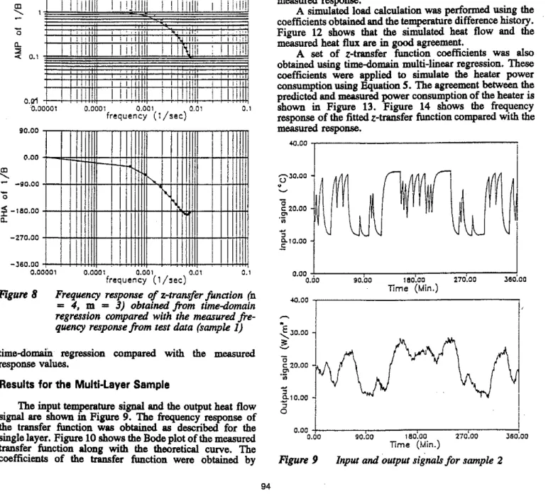
·Figure 3 shows the input and output sigusls for ssmple 1 after a periodic condition had been established. The frequency response of transfer function liB was obtained from·Equation 8 by performing a fast Fourier transform on input and output signals. The resulting frequency response, after normalizing to the stesdy-state U-value, is shown in ;the Bode plots ofFigure.4 along with the theoretical curve.

The theoretical derivation of frequency response ·is given in Appendix B. The agreement between the theoretical and experimental response .is good.

Although the frequency response function, .H(w), de-picted by the Bode plot is very useful, :the z-transfer function form is required for load calculation. To determine •the z-transfer function coefficients, a multi-linear regression computation was performed to fit z-transfer function coefficients to the frequency response data. For each chosen :frequency, two equations (the real component and the imaginary component of the transfer function) were written, ,plus one equation for the stesdy-state condition (see

Appen-dix A). The coefficients obtained are given in Figure

S,

which shows the frequency response of the derived

z-·transfer·function compared to. the measured response. These ·Coefficients were used to simulate the response (using Equation S) to the input signal for the test. Figure 6 shows ·the simulated response compared to the measured output. Multi•linesr regression was also.applied directly to the time ·domsin data. Figure 7 .shows the measured power con-. sumption of the heater along with the predicted consumption

using Equation S and coefficients ·from .the time domsin. The results show good agreement. Figure 8 plots the frequency response for the z-transfer function obtained by

93 - Ootr:uhlu:a • • ·• ·• ·• ·MIICSI.IfiiQ

·'"'

' ' ' I I _'

I

I

HI

I I. I

I

·JI,

I ' I I i

'WI)'

I 0.1

''Y

I I

· ·

I Ill

. ' . .ll..

ｾ＠

'

'

I :I I ｯＮｧＺｯｾ＠ JOI ·

I

i!

. ·;,:;,: •01

_{·o:. "}

.ii:.ll 0.1 ro '-90.00 O;OD ... -eo.oo 0 ｾ＠ -tao.oo "--21'0 . .00 ' :1 -:560.00 o;oaoot Figure4

"'

'

ｾ＠ ｾ＠

ｾ＠

-

0 ll.. 0.1 ｾ＠ 90.00 ｾ＠ 0.00 .e:_ ｾ＠ ｾ＠ Q-180.00 ｾ＠ 0... -270:00 -J60.00 o;·oaoat FigureS ;Frequency ( 1/sec)

,,,,

II

IIIII IIIII I /.·Ill

111111:-J

I !1.1111

!

111:11

I

1·11:11111

Jill

ｾＱｗｊ＠

1.1·111 II

.I''

II

!!II

.I

jl.'li

_I

Ill

Ill

!

II

I

ri

I

111::

111 1 1 11 1

1

I '

111.1

li!illl\ii·lllil

0.000·1 -0.001 -0,"0-1 0.'1 Frequency . (1 /sec)

Frequency ·response from test data for sample

1

I

a.• • •- • Ｚｍ･･ｾｳｵｲ･､＠ .-Fitted 0.0001 .0.001 Frequency (1/sec) 0.1

l

. '.1 ' : '.

I

•1

I

I .Ill

II'

I

11'11

I

IIIII

.I'

I

I

I I

''

I' I

_I

I

_'I

'

l

!

•

I

r ; I . '

I I

'

_I

Iii

'

Jl

i

I

I

I

"

o:ooot a.oat .o.ot 0.1

Frequency (,1 /sec),

Frequency .response of z-tranifer function for

sample 1

(D.

=

1

min,

Bo

=

0.0, a1

=

0.17,

• • • • • Slmulotlon - Meosur11d 180.00

.,.---·---o.---,

CD 135.00 •

'

0 90.00

..

.·

0.00

-1---.---,---,---1

0.00 18.00 36.00 54.00 72.00 Time (min.)

Figure 6 Simulated load for sample 1 (a = 1 min; the coefficients used are the same as in Figure 5)

90.00 0.00 ｾ＠ - -90.00 0 ｾ＠ -1BO.OO 0. -270.00 -360.00

I

I

I

!'...

• • • • • 1.le::::o.orl!d - - .=l:ac;rusion

!'-I !'-I

II II

I

0.00001 0.0001 0.001 0.01 0.1 frequency ( 1 /oec)

Figure 8 Frequency response of z-transfer function (n

=

4, m

=

3) obtained from time-domain regression compared with the measured fre-quency response from test data (sample 1)

time-domafu. regression compared with the messured response values.

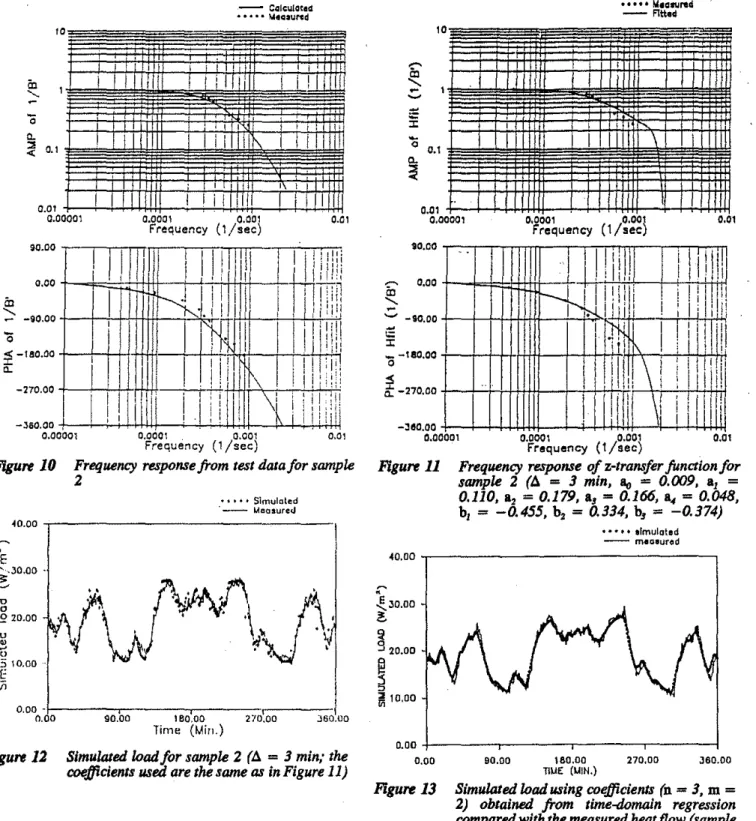
Results for the Multi-Layer Sample

The input temperature signal and the output hest flow signal are shown in Figure 9. The frequency response of the transfer function was obtsined as described for the single layer. Figure 10 shows the Bode plot of the messured transfer function along with the theoretical curve. The coefficients of the transfer function were obtsined by

94 180.00

o----CD I 35.00 •

'

0 90.00 • "0

_§

<5.00-

ｾＨ＠

• • • • • Slmulotion - lAaoaured o.oo

·r---,---,---,---0. 0 18.00 36.00 54.00 72.00 Time (min.)

Figure

7

Simulated load using coefficients (n = 4, m =

3) obtained from time-domain regression compared with the measured heat flow (sample 1) (a= 1 min)

performing multi-linear regression to the frequency

re-sponse data; Figure 11 shows the frequency rere-sponse plot for the derived z-transfer function compared with the measured response.

A simulated load calculation was performed using the coefficients obtained and the temperature difference history. Figure 12 shows that the simulated hest flow and the messured hest flux are in good agreement.

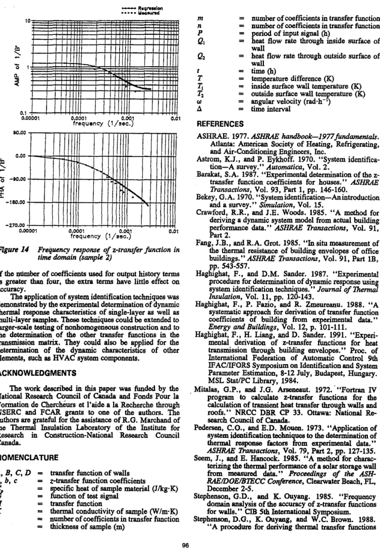
A set of z-transfer function coefficients was also obtsined using time-domain multi-linear regression. These coefficients were applied to simulate the hester power consumption using Equation S. The agreement between the predicted and messured power consumption of the hester is shown in Figure 13. Figure 14 shows the frequency response of the fitted z-transfer function compared with the measured response. 40.00 , - - - ; 0 c: 20.00

"'

'ii ｾ＠

,

.5'0.00

0.00 _0.00

-±-=---==---==---==:---:::i-

_{90.00 1 !10.00 270.00 360.00} Time (Min.) 40.00 . , . - - - ,

ｾｊｏＮｏｏ＠

ｾ＠ 0 c:: 20.00

"'

'ii '5 ..9-1 0.00

,

0

0.00 _o.oo

+-:---.,..,..,----::=---==--=::!

_{90.oo 1ao.oo 21o:oo Jso:oo}

Time (Min.)

90.00 0.00 1D :::- -90.00 0

:e

-11!0.00 a. -270.00

Ill

I

I

I I

I

I

I

I

I

- ｃＮ｡ｬ｣ｗｯｾ･､＠ • • • • • Meaaured I

I I!

II II

/I

I

I !I Iii

I

, ' I

_tW:H:

I

'I '

I

: nm

ｾｩｩ＠

',,, !

I

I· i

ll:i

.I

I I

II'%

lj

I

I

I

I

I li

il

It

IiI

; 11,11 II'· I 1•1

/I

I

I

_I

_!

I:

_l'i

-"'

i

' i I :i!1

'

'' ｉＡＬﾷﾷｾｾ＠ ' I I : i

',

I

' ' I

''

'I

I

-360.00 0.00001

I

_'

!

i

! I

_''

\''il:il

1 ｾ＠ , , • :

n

i

I!

i

iii O.OOOt 0.001 0.01 Figure

10

Frequency (1/sec)

Frequency response from test data for sample 2 • • • • • Simulated ·-Measure<.! <O.OO , - - - , o.oo -J:----::-cc:---=-:-:---:::::r-:-::----:-:-:1 0.00 90.00 I BO.OO 270.00 J60.00 Figure 12 Time (Min.)

Simulated load for sample 2 (fl. = 3 min: the coefficients used are the same as in Figure

11)

DISCUSSION AND CONCLUSIONS

The frequency response was obtained from tests using a BMFS signal as input and applying Fourier aoalysis to the resulting input/output signals. The results agreed reasonably well with the theoretically calculated response for both the single-layer aod multi-layer samples, especially at lower frequencies.

Binary multi-frequency signals have several advaotages as ao excitation for system identification. They are easy to produce, they cao

minimize

the distorbaoce to the system under test, they are efficient in concentrating power at appropriate frequencies, aod they show a clear indication of the frequencies for which response is being obtained.

95 10.00 -- o.oo 1D

'

-- -90.00

-i

- -180.00 0 ｾ＠ 0.. -270,00

--i

I

111

i!

I

I

JJ•

11,1

ｾ

ＱＱ

_{ＱＡＱＱＱＱ＠}

I

I

1

.Jiilili

l}lli

I. ·: . ;

_{\ f} I

I

I

!

ill!!

\I

'

I

\I

I

I

IiI

ill

• I '

I!"'

!

i

I I !I I

i ;

I

I

I

i1

I I• t

I

I I'

: IIi

11!1

: iII'

•I ,I

: I!

I

!!

: ! lit · -::!1!0.00 0.00001 0.0001

m

0.001 frequency ( 1/sec)

i

IIi

0.01 Figure 11

ｾＳＰＮＰＰ＠

ｾ＠

ｾ＠

20.00

ｾ＠

"

ｾ＠ 10.00

Frequency response of z-transfer function for sample 2 (fl. = 3 min,

a,

=

0.009,

a1 =

0.110,

a, =

0.179,

a, =

0.166,

a₄ =

0.048,

b, =

-0.455,

b,

=

0.334,

b,

=

-0.374)

• • • • • elmuloted - meaeur4d 0.00

+ - - - , - - - , - - - - , - - - - l

o.oo 90.00 160.00 270,00 J60.00 llUE (UIN.)

Figure 13 Simulated load using coefficients (n = 3, m =

2) obtained from time-<Wmaln regression compared with the measured heat flow (sample

2)

The z-traosfer function coefficients were obtained in two ways-by fittin!! coefficients to the measured frequency response and by fitting coefficients directly using regression aoalysis in the

time

domain. Both of these techniques ptoduced a z-transfer function that simulated the thermal response of the sample; the predicted heat flow rate (Q1) agreed very well with the measured value. Both methods gave good agreement even though the number of temper-ature and

heat

flow history terms is less

thao

four. This confirms the claim by Stephenson aod Ouyaog (1985) that

Ｐ

_{ｯＮｾｯＧ［ｏ｜＠}

80.00 o.oo 0 -ao.oo

l

-180.00 -270.00 0.00001

'

•01

ＨＱｾ＠

r-....

f-.

ｾ＠

0.0001 O.OQ_1 froquoncy (1/soc.)

,

I

0.01

Figure 14 Frequency response of z-transfer juncJion In time domain (sample 2)

if the nlimber of coefficients used for output history terms is greater than four, the extra terms have little effect on

accuracy.

The application of system identification techniques was demonstrated by the experimental determination of dynamic thermal response characteristics of single-layer as well as multi-layer samples. These techniques could be extended to larger-scale testin& of nonhomogeneous construction and to the determination of the other transfer functions in the transmission matrix. They could also be applied for the determination of the dynamic characteristics of other elements, such as HV AC system components.

ACKNOWLEDGMENTS

The work described in this paper was funded by the National Resesrch Council of Canada and Fonds Pour Ia Forination de Chercheurs et I' aide a

Ia

Recherche through NSERC and FCAR grants to one of the authors. The authors are grateful for the assistsnce ofR.G. Marchand of the Thermal Insulation Laboratory of the Institute for Resesrch in Construction-National Research Council

Canada.

NOMENCLATURE

A,B,C,D

₌

transfer function of walls

a,

b,

c

₌

z-transfer function coefficients

?

=

specific hest of sample material (J/kg· K)

=

function of test signal

H

₌

transfer function

K

₌

thermal conductivity of sample ryf/m· K)

k

₌

number of coefficients in transfer function

L

₌

thickness of sample (m)

96

m = number of coefficients in transfer function

n

= number of coefficients in transfer function

p

₌

_{period of input signal (h)}

Q, = hest flow rate through inside surface of wall

Q, = heat flow rate through outside surface of wall

I = time (h)

T = temperature difference (K)

11

= inside surface wall temperature (K)

12

= outside surface wall ｴ･ｾ･ｲ｡ｴｵｲ･＠ (K)

w

= angular velocity (rad·h- )

.1 = time interval REFERENCES

ASHRAE. 1977. ASHRAE handbook-1977 fundamentals. Atlanta: American Society of Resting, Refrigerating, and Air-Conditioning Engineers, Inc.

Astrom, K.J., and P. Eykhoff. 1970. "System identifica-tion-A survey." Automatica, Vol. 2.

Barakat, S.A. 1987. "Experimental determination of the z-transfer function coefficients for houses." ASHRAE

TransacJions, Vol. 93, Part 1, pp. 146-160.

Bekey, G.A. 1970. "Systemidentification-Anintroduction and a survey." Simulation, Vol. 15.

Crawford, R.R., and J.E. Woods. 1985. "A method for deriving a dynamic system model from actual building performance data." ASHRAE TransacJions, Vol. 91, Part 2.

Fang, J.B., and R.A. Grot. 1985. "In situ measurement of the thermal resistsnce of building envelopes of office buildings." ASHRAE TransacJions, Vol. 91, Part lB, pp. 543-557.

Haghighat, F., and D.M. Sander. 1987. "Experimental procedure for determination of dynamic response using system identification techniques." Journal of 1hermal

Insulation, Vol. 11, pp. 120-143.

Haghighat, F., P. Fazio, and R. Zmeureanu. 1988. "A systematic approach for derivation of transfer function coefficients of building from experimental data."

Energy and Buildings, Vol. 12, p. 101-111.

Haghighat, F., H. Liang, and D. Sander. 1991. "Experi-mental derivation of z-transfer functions for best transmission through building envelopes." Proc. of International Federation of Automatic Control 9th IF ACIIFORS Symposium on Identification and System Parameter Estimation, 8-12 July, Budapest, Hungary. MSL Stat/PC library, 1984.

Mitalas, G.P., and J.G. Arsenesut. 1972.- "Fortran IV · program to calculate z-transfer functions for the calculation of transient best transfer through walls and roofs." NRCC DBR CP 33. Ottawa: National Re-search Council of Canada.

Pedersen, C.O., and E.D. Mouen. 1973. "Application of system identification techniques to the determination of thermal response factors from experimental data."

ASHRAE TransacJions, Vol. 79, Part 2, pp. 127-135. Seem,

J.,

and E. Hancock. 1985. "A method for charac-terizing the thermal performance of a solar storage wall from measured data." Proceedings of tlu!

ASH-RAEIDOEIBTECC Conference, Clearwater Beach, FL, December 2-5.

Stephenson, G.D., and K. Ouyang. 1985. "Frequency domain analysis of the accuracy of z-transfer functions for walls."

em

5th International Symposium. Stephenson, D.O., K. Ouyang, and W.C. Brown. 1988.

for walls from hot-box test results."

IRC

Internal Report No. 568. Ottawa: National Research Council of

Canada.

Van den

Bos,

A. 1967. "Construction of binary multi-frequency signals.'' Proc. of International Federation of Automatic Control Symposium.

APPENDIX A

Derivation of z-Transfer Function Coefficients from Frequency Response Data

The :.-transfer function is given in the form:

- J -2 -II

H(z.) •

Do

+ a1 z +a,

z.

+ ... + a. z

1

b

-1

b

-2

b -·

(A1)

+ 1.t + 2Z + ••• +

.z

where a1 and b1

are

:.-transfer function coefficients,

z-

1 is

an operator representing a

time

delay = Ill, and ll is the sampling time interval of the :.-transform. Since

z

=

tl",

Equation A1 can be expressed in Laplace notation:

H(s) •

Do

eo+ at e-A• + ｾ＠ ｾＭＲａＮｲ＠ + ••• +a,. ,-•A.r

1

+

b

₁

e" 4'

+

_b2e·2h

+ ... +

b.,e·•h

(A2) Substitutingjw

=

s,

Equation A2 becomes:

H("') =

ao

+at _{,-J.,A + ｾ＠ ,-2J"A} + .•.

+a,.

,-,.J.,A

1

+ bl ,-Jw4 + b2 e·7./d + ... +b., e·•Jd

(A3) Substitute

e·i""'

= cos (wll) - jsin (wll), and Equation A3 becomes:

H("') =

a

₀ +

a

₁ [cos("' ll) -)sin("' A)] +a, [cos(2"' A)- jsin 1 + b₁ [cos("' A) -)sin("' ll )] + b₂ [cos(2., A)- jsin(

... +a.[ cos(n"' A) -jsin(n"' A)

1

... + b.,[cos(m"' A)-jsin(m"' A)]

(A4)

1 1 u

1 cos(w

1) cos ( 2w1) -{11Rcos(w1)+111sin(u1))

0 -sin(u

1) -sin(2w1) [U8sin(w1)-111cos(u1))

1 cos {w

2) cos ( 2w2) -(Jt11cos(w2)+111sin(w2)] 0 -sin (w

2) ｳｩｮＨＲｷ［［ｾＩ＠ [1111sin(w2) Ｍｈ Ｑ｣ｯｳＨｷｾｽＩ＠

1 cos(wJ) cos{2w

3) •(1111COS (W3) +111sin (w3)) 0 -sin(w

3) -sin(2w3) (H11sin(w3) -111cos {w3))

1 COS (W

11) cos (2wK) -[U11cos(w11)+111sin(w11)]

a -sin(w

11) -sin(2W11) (ll11sin (w11)-111cos (w11) J

97

Because the frequency response, H, is a complex function, it can be written in two parts: real component, H_{8 ,} and imsginary component, H1:

H(6l) = H•("') + jH_{1( " ' ) .} (AS)

Equating Equations A4 and A5 yields:

HR(6l) s ao+a,cos(6lA)+a,cos(2.,A)+ ... +a.cc - b₁[HR("') cos(.,A) + H₁(6>) sin(.,ll)]- ... - b.[HR("') cos(m6l A)+ H_1("') sin(m"' A)]

(A6)

H_1("') = -a₁sin(.,A) -a,sin(26lA)- ... -a.sin(n<

+ b₁ [HR( 6l) sin("' ll)- H_1("') cos("' A)] + ... + b.,[HR(.,) sin(m6l A)- H_{1( "')} cos(m6l A)] . (A7)

An additional equation can be written for the steady-state gain (w = 0). Therefore, N frequencies, 2 N+ 1 equations

can be obtained. Rewrite these equations in a matrix form (see below) where Wo = 0 is the steady-state condition at which Equation A3 reduces to

U= <Jo+a1+a,+ ... +a• 1 + b, + b2 + ... + b,.

(AS)

where

U

is the steady-state U-value. Equation AS can be given extra weight to ensure thet the :.-transfer function has the correct steady-state U-value.

Solving the matrix equation using multi-linear regres-sion techniques, the coefficients

a.

to

a.

and b1 to bm

can

be obtained. For statistical and probabilistic considerations, the number of frequencies, N, needs to be larger than the number (n+m) of coefficients to be determined. A compli-cation may arise when phase lags of 1SO' occur. Under this condition, the regression may produce negative values for

a,.

This

can

be prevented by forcing

a.

to zero in Equations A6 and AS. u u -[UK cos { 2w 1) +111s in ( 2w1) ]

•,

IIR '"·\) {URsin ( 2w 1 )-U1cos ( ＲｷＬｾＩＩ＠

•,

111 (w1)

- (H"cos ( 2wa) +111sin ( 2w2) l

•,

""' Ｈｷ［［ｾＩ＠ (U

11sin {2w2)-111cos { 2wz) )

•,

H1(wil)

- (HRCOS ( 2wl) +11_{1sin ( 2W3) ]} ( 11 11sin ( 2w3) -111cos ( 2w3) ]

•

" b

•

b, -[11 11cos(2w11)t111sin(2W11)) b HR (wN) (H 11sin(2wN) -ll1cos (2w11)]

.

11 1 (w11)

:I

:1

I

il

J

lj

APPENDIX B

The transmission matrix relates the temperatures aod the heat flows on both sides of the envelope, which is

in

the form of

｛ｾＺ｝ﾷ＠ ｛ｾ＠ ｾｬ｛ｩ｝＠

(Bl)

where

A, B, C, and D

are

transfer functions aod

are

given

in

hyperbolic functions as aod A(.r) =

｣ＺｯｳｨＨｬｾＩ＠

-·-.,, r:;,

B(.r) =

=:E

ｋｾ＠

D(.r) •

｣ＺｯｳｨＨｬｾＩ＠

K

«

=

-C,p

(B2)

where K, Cl"_ p, l, and

a

are

thermal conductivity, specific heat, densi•y, thickness, aod thermal diffusivity of the material, respectively.

For a multi-layer wall, the transmission matrix of the whole wall is to be expressed by the product of the trans· mission matrices of each layer of the wall, i.e.,

DISCUSSION

Dennis Loveday, Professor, Loughborough University, Department of Civil Engineering, Loughborough, Le1cestershire, UK: In what way does your input signal differ from that of a pseudo-raodom binary sequence (PRBS)?

98

The transmission matrix cao be rearranged to express surfsce heat flows as

response

aod the surface temperature

as

excitation: lS(S) __ 1_ I(S) I(S)

_1_-

A(S) I(S) I(S) (B4)

For a two-layer wall, the element of transmission matrix (Equation B4) is given as:

where

(BS)

The theoretical frequency response is obtained by substitu-ting

jw

for

s

in

Equation B4.

F.

Haghighat: In our study, a binary multi-frequency sequence was chosen as the input excitation signal. This type of signsl has several attractive characteristics for system identification compared to PRBS. It is easy to produce aod requires no complex waveform generator or precise control. It minimizes the disturbaoce to the system under test, aod it is efficient at concentrating power at appropriate frequencies.