Design of flexure-based motion stages for mechatronic systems via Freedom, Actuation and Constraint Topologies (FACT)

(1)

Design of Flexure-based Motion Stages for Mechatronic

Systems via Freedom, Actuation and Constraint Topologies

(FACT)

by

Jonathan Brigham Hopkins

M.S. Mechanical Engineering

Massachusetts Institute of Technology, 2007 B.S. Mechanical Engineering

Massachusetts Institute of Technology, 2005

MASSACHUSETTS INSTITUTE

OFCHIVES

ARCHNVES

SUBMITTED TO THE DEPARTMENT OF MECHANICAL ENGINEERING

IN PARTIAL FULFILMENT OF THE REQUIRMENTS FOR THE DEGREE OF DOCTOR OF PHILOSOPHY IN MECHANICAL ENGINEERING

AT THE

MASSACHUSETTS INSTITUTE OF TECHNOLOGY

SEPTEMBER 2010

@ 2010 Massachusetts Institute of Technology

The author hereby grants to MIT permission to reproduce and to distribute publicly paper and electronic copies of this thesis document in whole or in part

in any medium now known or hereafter created.

Signature of Author: ....

.

/.O. Certified by:

.... ,... ...

De ment of Mechanical Engineering August 24, 2010

Martin L. Culpepper Associate Professor of Mechanical Engineering

7)

S

i

upervisor

A ccep ted b y : ... . . ...

David E. Hardt Professor of Mechanical Engineering Chairman, Department Committee on Graduate Students

(2)

(3)

Design of Flexure-based Motion Stages for Mechatronic

Systems via Freedom, Actuation and Constraint Topologies

(FACT)

by

Jonathan Brigham Hopkins

Submitted to the Department of Mechanical Engineering on August 24, 2010 in Partial Fulfillment of the

Requirements for the Degree of Doctor of Philosophy in Mechanical Engineering

ABSTRACT

The aim of this thesis is to generate the knowledge required to (i) synthesize serial flexure systems and (ii) optimally place actuators using a comprehensive library of geometric shapes called freedom, actuation, and constraint spaces. These geometric shapes guide designers through the creative process of concept generation without compromising engineering rigor. Each shape rapidly conveys the mathematics of screw theory, projective geometry, and constraint-based design by visually depicting regions where constraints and actuators may be placed for synthesizing optimal flexure concepts. In this way, designers may consider every flexure concept that satisfies the desired functional requirements before selecting the final design. FACT was created to improve the design processes for small-scale flexure systems and precision machines. For instance, there is a need to create multi-axis nanopositioners for emerging three-dimensional nano-scale research/manufacturing. Through this work the following contributions were made: (1) the fifty freedom and constraint space types were found that may be used to synthesize both parallel and serial flexure concepts, (2) intermediate freedom spaces were created that help designers stack conjugated flexure elements to avoid or utilize underconstraint, (3) a twist-wrench stiffness matrix was created to model the elastomechanic behavior of flexure systems, (4) the twenty-six actuation spaces were found that help guide designers in placing actuators that minimize motion errors, and (5) a theory was created that determines the force and displacement actuator outputs for accessing a desired DOF once actuators have been placed. A serially conjugated lead screw flexure was designed using the

FACT design process and a parallel flexure system was built to validate the theory of actuation

described in this thesis.

Thesis Supervisor: Martin L. Culpepper

(4)

ACKNOWLEDGMENTS

I would like to thank all those who helped make this research possible. I first acknowledge God

whose hand is in all discoveries and whose love makes all things possible. I am also forever grateful to my devoted parents, Barbara and James Hopkins, who have sacrificed greatly for my education. A special thanks to my advisor, Professor Martin Culpepper, who tirelessly

motivated, guided and directed my efforts. This work would not have been possible without his patience and faith in me. I am grateful to the other members of my doctoral committee, Professors Sarma and Seering, who helped shape this research with their insights and suggestions. To Jan van Eijk, Jingjun Yu, and my dear friends in the Precision Compliant Systems Laboratory who offered their support, patience and correction, I am also in debt. And finally, I am grateful to NSF, Soliant Energy, and Novartis for providing funding during my time as a research assistant. Thank you all very much.

(5)

3.4.1 3 DOF Type 1...73 3.4.2 3 DOF Type 2...74 3.4.3 3 DOF Type 3...75 3.4.4 3 DOF Type 4...76 3.4.5 3 DOF Type 5...80 3.4.6 3 DOF Type 6...83 3.4.7 3 DOF Type 7...85 3.4.8 3 DOF Type 8...87 3.4.9 3 DOF Type 9...89 3.4.10 3 DOF Type 10...91 3.4.11 3 D O F Type 11 ... 93 3.4.12 3 DOF Type 12...95 3.4.13 3 DOF Type 13...97 3.4.14 3 DOF Type 14...99 3.4.15 3 D O F Type 15...101 3.4.16 3 DOF Type 16...103 3.4.17 3 DOF Type 17...106 3.4.18 3 DOF Type 18...107 3.4.19 3 DOF Type 19...108 3.4.20 3 DOF Type 20...110 3.4.213 DOF Type 21...111 3.4.22 3 DOF Type 22...112

3.5 Types within the 4, 5, and 6 DOF Column...114

3.6 Practical FACT Chart...114

CHAPTER 4: Optimal Actuator Placement...115

4.1 T echnical Scope...115

4.2 Fundamental Principles...115

4.2.1 Linking Motions to Actuation Forces...116

4.2.2 Geometric Shapes as Design Tools...117

4.3 A ctuation Space...119

4.3.1 Examples of Actuation Space...119

4.3.2 Actuation Space as a Design Tool...120

4.4 Actuator Placement and Outputs...122

4.4.1 Force-based Actuation...123

4.4.2 Displacement Actuation...125

4.5 Twist-Wrench Stiffness Matrix...125

4.5.1 Defining the Twist-Wrench Stiffness Matrix...125

4.5.2 Derivation of the Twist-Wrench Stiffness Matrix...127

4.6 Numerical Example...128

4.6.1 Calculating the Flexure System's TWSM...128

4.6.2 Calculating the System's Actuation Space...130

4.6.3 Calculating Force and Displacement Ratios...132

(7)

CH A PTER 5: C onclusions...136

5.1 Thesis C ontributions...136

5.2 Future W ork ... 137

APPENDIX A: Derivation of Spaces within Chart...139

APPENDIX B: Actuation Space MATLAB Code...183

(8)

LIST OF FIGURES

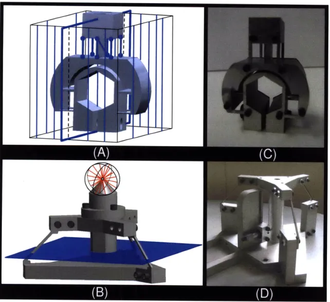
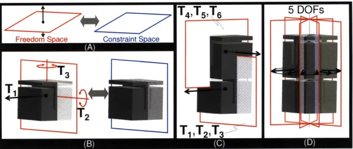
Figure 1.1: Geometric shapes (A) and (B) may be used to synthesize and actuate flexure systems

(C ) an d (D )...16

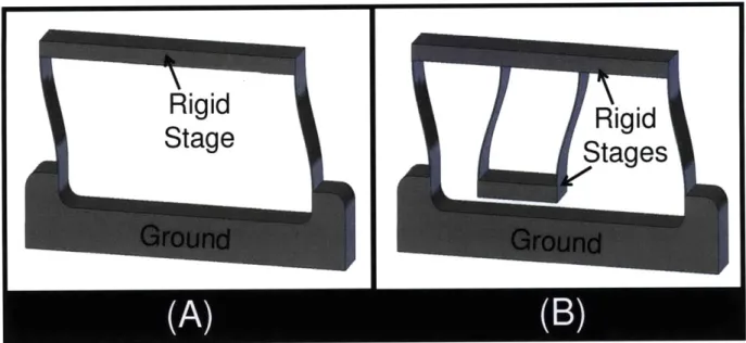
Figure 1.2: Example of a parallel flexure system (A) and a serial flexure system (B)...17

Figure 1.3: Example flexure system with desired rotation (A), intuitive actuator placement with shifted rotation that yields error (B), correct actuator placement (C)...21

Figure 1.4: Twist parameters defined (A), rotation twist (B), translation twist (C), screw twist (D )... . . .. 22

Figure 1.5: Example flexure system with two rotational DOFs (A) and (B). The flexure system's freedom space is a disk of rotations (C)...23

Figure 1.6: Wrench parameters defined (A). Color coded wrench types (B). Pure force wrenches modeling long slender constraints (C). Pure force wrenches modeling thin blade flexures (D )... . . .. 24

Figure 1.7: Eight wrenches that model the system's constraints (A). Mathematical and practical system constraint space (B). System constraints lie within its constraint space (C)...25

Figure 1.8: Complementary twist and wrench parameters (A). Uniquely linked freedom and constraint space pair for the example flexure system (B)...27

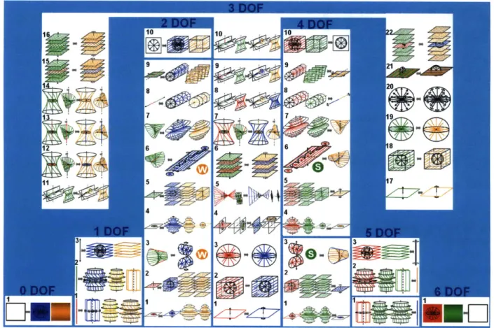
Figure 2.1: Mathematically comprehensive FACT chart...30

Figure 2.2: Practical FACT chart for flexure synthesis...31

Figure 2.3: Flexural elements in parallel (A) and in series (B)...32

Figure 2.4: 3 DOF parallel flexure system (A). 5 DOF stacked serial flexure system (B)...34

Figure 2.5: 3 DOF Type 1 freedom and constraint spaces (A). Spaces imposed on the 3 DOF parallel flexure module (B). Intermediate freedom spaces (C) sum together to produce the 5 DOF freedom space of the serial flexure system (D)...35

Figure 2.6: 5 DOF Type 1 freedom and constraint space (A). Spaces imposed on the 5 DOF wire flexure (B). Wire flexure and serial flexure chain are kinematically equivalent (C). Two kinematically equivalent flexure systems (D)...37

Figure 2.7: Steps of the FACT design process...38

(9)

Figure 2.9: The desired motions that should be imparted on the hex nut by the flexure system

(A) and the freedom space of those desired motions (B)...42

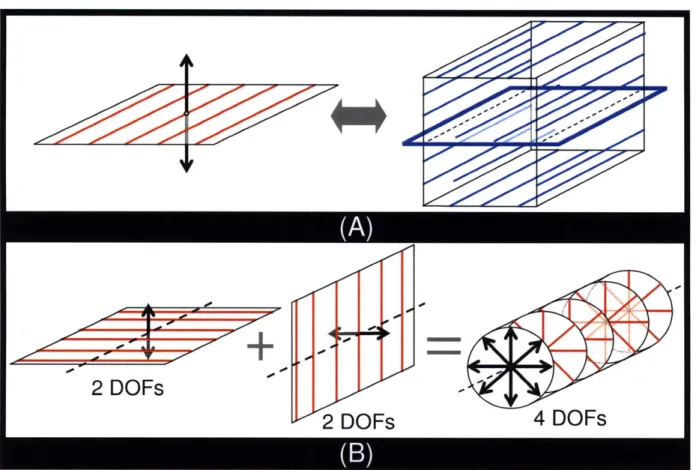
Figure 2.10: Freedom and constraint space of 2 DOF Type 2 (A). Two intermediate freedom spaces sum together to generate the freedom space of the system (B)...44

Figure 2.11: Geometric constraints shape the ground and stage designs (A). The ground and stages shown with the desired DOFs (B)...45

Figure 2.12: Orientation of the first intermediate freedom space (A) and its complementary constraint space (B). Flexible constraints selected from the constraint space connect the main stage to the intermediate stage (C)...45

Figure 2.13: Orientation of the second intermediate freedom space (A) and its complementary constraint space (B). Flexible constraints selected from the constraint space connect the intermediate stage to the ground (C)...46

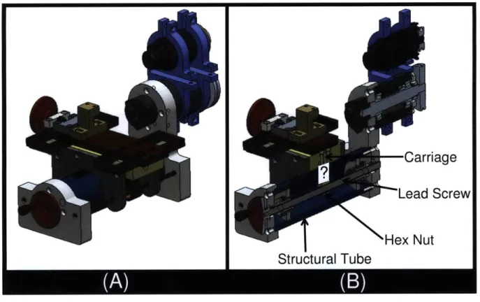
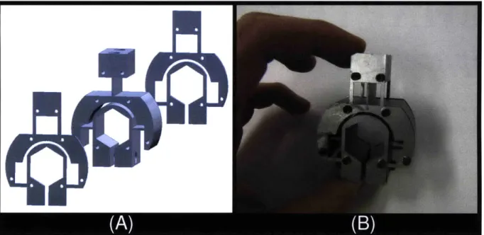
Figure 2.14: The flexure consists of three planar pieces (A). The final lead screw flexure (B)..47

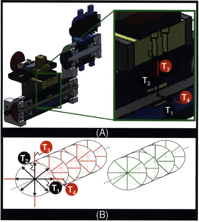
Figure 2.15: The four DOFs of the lead screw flexure (A), (B), (C), and (D)...47

Figure 3.1: Freedom space of 0 DOF Type 1...49

Figure 3.2: Constraint space of 0 DOF Type 1...50

Figure 3.5: Parameters that define the wrenches within the constraint space of 1 DOF Type 1..51

Figure 3.8: Parameters that define the constraint lines within the constraint space of 1 DOF T y p e 1...54

Figure 3.13: Parameters that define the wrench lines within the constraint space of 2 DOF T ype 1... . . 57

(10)

Figure 3.16: Parameters that define the wrench lines within the constraint space of 2 DOF

T ype 2 ... . 59

Figure 3.21: Parameters that define the constraint lines within the constraint space of 2 DOF T ype 4 ... . 62

Figure 3.24: Parameters that define the constraint lines within the constraint space of 2 DOF T ype 5 ... . 64

Figure 3.27: Parameters that define the blue disks within the constraint space of 2 DOF T ype 6 ... . 67

Figure 3.30: Parameters that define the blue constraint lines (A) and orange wrench lines (B) within the constraint space of 2 DOF Type 7...69

(11)

Figure 3.43: Freedom space of 3 DOF Type 4A...76

Figure 3.44: A set of screws of the same pitch value that lie on the surface of a hyperbolic paraboloid and belong to the freedom space of 3 DOF Type 4A...77

Figure 3.45: Constraint space of 3 DOF Type 4A...78

Figure 3.46: Freedom space of 3 DOF Type 4B...79

Figure 3.47: Constraint space of 3 DOF Type 4B...80

Figure 3.48: Freedom space of 3 DOF Type 5A... 81

Figure 3.49: A set of screws within the freedom space of 3 DOF Type 5. The screws within this set possess the characteristic screw's pitch value...82

Figure 3.50: Constraint space of 3 DOF Type 5A...83

(12)

3.71: Freedom space of 3 DOF Type 16...104

3.72: A cylindroid from the freedom space of 3 DOF Type 16...105

3.73: Constraint space of 3 DOF Type 16...106

Figure Figure Figure Figure Figure Figure Figure Figure Figure Figure Figure Figure Figure Figure Figure D O F T ype 17...106 3 DOF Type 17...107 D O F T ype 18...107 3 DOF Type 18...108 D O F T ype 19...109 3 DOF Type 19...109 D O F T ype 20...110 3 DOF Type 20...110 D O F T ype 21...111 3 DOF Type 21...111 D O F T ype 22...112 3 DOF Type 22...113

Figure 4.1: Parameters defined for a desired twist (red line with a circular arrow) that is optimally actuated by a wrench (blue arrow)...117

Figure 4.2: Three independent DOFs represented as twists, Ti, and their corresponding actuator placements represented as wrenches, Wi (A). Freedom and actuation spaces of the flexure system (B )...118

Figure 4.3: A flexure system with a planar freedom space (A) and a box-shaped actuation space of parallel lines (B )...119

Figure 4.4: A flexure system with a planar freedom space of parallel rotation lines (A) and a disk-shaped actuation space (B)...120

Figure 4.5: The twenty-six actuation spaces that pertain to systems actuated by linear actu ators...12 1 Figure 4.6: A triangular actuation scheme for accessing every rotation in the sphere with minimal error (A), and the corresponding actuator force ratio for accessing the particular rotation, T (B )...124

Figure 4.7: Parameters that define the TWSM, (A) and (B)...127 Freedom space of 3 Constraint space of Freedom space of 3 Constraint space of Freedom space of 3 Constraint space of Freedom space of 3 Constraint space of Freedom space of 3 Constraint space of Freedom space of 3 Constraint space of 3.74: 3.75: 3.76: 3.77: 3.78: 3.79: 3.80: 3.81: 3.82: 3.83: 3.84: 3.85:

(13)

Figure 4.8: Numerical example flexure system with parameters (A), and actuator setup with param eters (B )...129 Figure 4.9: Experimental flexure setup for measuring error, e (A), and the CMM used to

measure the twists imposed by the micrometer (B)...134 Figure 4.10: Experimental (A) vs. theoretical (B) errors of the probe's tip...135 Figure A. 1: Twist configurations that generate every type within the 2 DOF column...140 Figure A.2: All twist configurations that build off of the configuration from Figure A. lA to

generate types within the 3 DOF column...141 Figure A.3: All twist configurations that build off of the configuration from Figure A. lB to generate types within the 3 DOF column...142

(14)

LIST OF TABLES

Table 3.1: Freedom space color code for various twist types...48 Table 3.2: Constraint space color code for various wrench types...48

(15)

CHAPTER 1:

Introduction

This chapter provides a discussion of the purpose, importance, and impact of this research. The background principles that are necessary to understand the contributions of this work are briefly reviewed and an overview of the content of this thesis is provided.

1.1 Research Objectives

The purpose of this thesis is to generate the principles required to (i) synthesize multi-degree of freedom (DOF) flexure systems and (ii) optimally place their actuators. These principles are embodied in the form of geometric shapes like those shown in Figure 1. 1A-B that help designers visually identify all the possible regions where constraints and actuators may be placed in order to achieve desired motions. These shapes - called freedom, actuation, and constraint spaces

-enable designers to rapidly consider all the possible flexure concepts before selecting the concept that best satisfies the system's functional requirements. The flexure design process that utilizes these shapes is called Freedom, Actuation, and Constraint Topologies (FACT). Examples of multi-DOF flexure systems designed using FACT are shown in Figure 1.1 C-D.

Flexure systems have been used as precision machine elements for over a century [1-8] due to their exceptional resolution characteristics, their low-cost characteristics, and the ease with which they may be fabricated. Flexure systems continue to be important to conventional precision applications. For example they are commonly used within optical manipulation stages, precision motion stages and as general purpose flexure bearings. More recently, flexure systems have become attractive for use in motion stages for nanomanufacturing equipment [9-10], instruments that are used in scale research/manufacturing [11-15], and micro- and nano-manipulators [16-18]. These instruments and devices typically require the capability to move in four to six axes with nanometer-level resolution.

(16)

Figure LI: _{Geometric shapes (A) and (B) may be used to synthesize and actuate flexure}

systems (C) and (D).

1.1.1 Serial Flexure Synthesis

All flexure systems fall under two categories - parallel or serial. Parallel flexure systems consist of a single rigid stage that is connected directly to ground by non-conjugated flexible elements. Serial flexure systems consist of nested parallel flexure systems that are stacked together. Figure 1.2 shows a parallel and serial flexure system. The principles needed to synthesize parallel flexure systems are provided in Hopkins [19-21]. A major objective of this thesis is to generate the principles needed to synthesize serial flexure systems.

(17)

Figure 1.2: Example of a parallel flexure system (A) and a serial flexure system (B).

The synthesis of multi-DOF parallel flexure systems is difficult because there are typically many flexural components. It is difficult for designers to keep track of (i) the relative, three dimensional orientations of the flexural constraints, (ii) the orientation of the permitted motions, and (iii) the three dimensional relationships between each constraint and the permissible motions. Even if an expert designer is capable of the preceding, the task of synthesizing a multi-DOF serial flexure system becomes more difficult as extra stages are stacked on top of each other. The kinematics, elastomechanics, and dynamics of each stage are influenced by the kinematics, elastomechanics, and dynamics of the proceeding stages in the serial chain. The task of synthesizing most serial flexure systems is, therefore, very difficult for flexure system designers that rely on intuition and motion visualization capabilities alone.

The existing body of published flexible mechanism design knowledge provides little information or guidance as to how to synthesize three dimensional, multi-DOF, serial flexure systems. The three most common approaches for designing flexible mechanisms include constraint-based design (CBD), the pseudo-rigid body model (PRBM), and topological synthesis. Constraint-based designers have developed rules of thumb for synthesizing simple, planar, flexure systems using well known flexural elements as building blocks [22-24]. Pseudo-rigid body modeling models compliant mechanisms (CMs) as analogies to rigid-link mechanisms

[25-27]. The rigid analog is then modeled using pre-existing rigid mechanism theory and the

principle of virtual work to ascertain its kinematic and elastomechanic properties. The PRB .. .. ... : ... :: ... .. ....

(18)

model has been used to design precision elastic mechanisms [28-29] and many consumer products. The primary aim of PRBM is to model, rather than synthesize, and so it is not ideally suited to solve the problems that are the target of this thesis. Topological synthesis is based upon computer algorithms that examine a starting shape for a compliant mechanism and then determines how to add/subtract material in order to create concepts that satisfy performance specifications [30-32]. In this method, the computer makes the design decisions that determine the layout of the rigid and flexible elements. This approach is effective for rapid synthesis of non-precision compliant mechanisms for robotics, MEMS and aeronautics. Unfortunately, topology synthesis is not readily applied to solve most precision flexure design problems. The reason for this is that the knowledge needed to integrate the specialized precision design rules with topological synthesis does not currently exist.

The ability to synthesize serial flexure systems is important because of their unique capabilities and advantages over parallel flexure systems. First, serial flexure systems are capable of permitting DOFs that are not possible for parallel flexure systems. A flexure system, for instance, that must permit only three independent translations, i.e. x-y-z, is only possible for a serial flexure system. The reason for this fact is that the moment a single flexible constraint is connected directly from a stage to ground, the stage looses one of its three translations along the constraint's axis. Parallel flexure modules must therefore be stacked in series to achieve three translations. Second, serial flexure systems may be designed to possess larger ranges of motion than same-size parallel flexure systems. Note that the serial flexure system from Figure 1.2 is the same size as the parallel flexure system shown, but the serial flexure system's stage is capable of moving twice the distance of the parallel flexure system's stage. Third, serial flexure systems may be designed to reduce parasitic errors. The parallel flexure system's stage from Figure 1.2 does not possess a perfect translational DOF. The stage follows an arc-like path over its range of motion. The stage of the serial flexure system moves along a "straighter" path because the vertical components of the opposing arc motions of the two rigid stages cancel.

A number of applications require the advantages that are inherent to serial flexure systems.

Compliant transmissions that amplify or attenuate forces or displacements are generally serial flexure systems because they consist of at least two stages-an input stage and an output stage. Six-axis, flexure-based nanopositioners must also be serial flexure systems if they are to achieve all six DOFs with comparable stiffness characteristics. Furthermore, some kinematically

(19)

equivalent serial versions of parallel flexure systems may be designed with (i) better elastomechanic characteristics, (ii) better dynamic characteristics, (iii) greater load capacities, and (iv) increased resistance to buckling.

The results of this thesis will enable one to consider all the possible ways of synthesizing serial flexure systems that possess any desired DOFs. A comprehensive library of geometric shapes has been created that links serial flexure designs to desired motions. These "graphical" representations of flexure performance enable one to understand what a flexure should look like if one wishes to achieve certain motion characteristics. After selecting the right design via these shapes, designers may use screw theory to tune and optimize a concept for specific design requirements. This method helps designers ascertain when it is best to use a serial or a parallel flexure system for a given application. New design rules have been found for serial flexure systems. These rules enable designers to rapidly identify concepts that possess desired symmetry, load capacity, and constraint redundancy. They may also be used to optimize the layout of a flexure system so that one may achieve the best flexure system's stiffness and dynamic characteristics.

1.1.2 Optimal Actuator Placement

Precision engineers take great care to model, design, and fabricate flexures such that they exhibit low (often nanometer-level) error motions. It is equally important to place the actuators properly, as an improper layout may cause additional errors (100s to 1000s of nanometers). The optimal actuator placement depends upon coupling of many design parameters and requirements. This coupling presents a complex problem that is not suitably addressed by intuition. It is necessary to have tools/principles that link actuator placement and flexure performance, thereby enabling a designer to set the best layout.

This thesis contains these tools and principles. A mathematical basis is introduced that may be used to determine the best layout for actuators. This information is then encapsulated within geometric shapes that designers may use to visualize the best locations to place actuators. This quantitative/qualitative combination enables rapid actuator layout during concept design, and the modeling that may be used to perform concept optimization and refinement. This approach enables designers to (i) visualize the regions wherein actuators should be placed so as to

(20)

minimize errors, (ii) guide designers in selecting these actuators to maximize the decoupling of actuator inputs, and (iii) determine actuator forces and displacements that actuate specific degrees of freedom.

The placement of actuators is a generic problem that is relevant to flexible mechanism design. This problem has been a topic of study in structure and robotic design [33-40], but little work has been directed towards the unique requirements of precision flexure systems, specifically those associated with thermal, vibration, fabrication, parasitic, and other error sources.

Parasitic errors are the deviations from a stage's intended motions where the magnitudes of these errors are linked with the magnitudes of the stage's intended motions. Parasitic errors that result from incorrectly actuating a flexure system are systematic, and may therefore be easily characterized by standard error mapping techniques [41-44]. For six DOF flexure systems, error mapping may be used to calibrate the machine via mechanical tuning or active control. For flexure systems with less than six DOFs, errors in non-actuated directions are not easily addressed. It is, therefore, important to know how to arrange the actuators to reduce these errors.

Proper actuator placement depends upon flexure geometry and material properties, therefore the process of specifying actuator placement should occur in early-stage design. In this approach, screw theory is used to generate three dimensional shapes, called actuation spaces, which may be used to visualize the best actuator placement.

One must consider the three dimensional geometries, motions, and deformations of the elastic elements in order to determine the best actuator placement. An experienced designer is not always guaranteed to find the best actuator placement via intuition. The thesis presents a tool that makes it easier for designers to consider all important aspects of the problem, and therefore select the best actuator placement.

The limitations of intuition are demonstrated via the following example. Suppose one wished to rotate the stage in Figure 1.3A about the dotted line that intersects a probe's tip. Engineers would typically intuit that the best actuator placement is that shown in Figure 1.3B. The detail in Figure 1.3B shows that this actuator placement yields a rotation about a line (solid) that is shifted from the desired line (dotted). This shifted rotation causes the probe's tip to displace with an error as shown in Figure 1.3B. If the flexure elements behaved as ideal constraints with infinite stiffness along their axes (this is often how they are visualized), this shift

(21)

would not occur. In reality, the flexure elements exhibit deformations, e.g. stretching along their axis(es) of constraint, that yield non-ideal motions that manifest as parasitic errors. These deformations cannot be predicted via constraint-based design principles. Later in this thesis, the twist-wrench stiffness matrix (TWSM) will be provided. This matrix may be used to determine that the best actuator placement is that shown in Figure 1.3C.

Error

Probe's

-.

Tip

_A

Figure 1.3: Example flexure system with desired rotation (A), intuitive actuator placement with shifted rotation that yields error (B), correct actuator placement (C).

1.2 Fundamental Principles

This section reviews the basic principles necessary to (i) synthesize parallel flexure modules using geometric shapes and (ii) model actuator placements. In following chapters these principles will be applied to (i) the synthesis of serial flexure systems and (ii) the optimal placement of actuators that minimize error.

1.2.1 Modeling Motions via Screw Theory

All small motions may be modeled as a 6x1 vector called a twist [45-48]. A twist may be

visualized as a line about, or along, which a stage rotates and/or translates. The pitch of a twist is defined as the ratio of the distance a stage translates along the twist's axis to the coupled rotation about this axis. A general displacement twist, T, is defined as:

T=[AO 8]' =[AO ((cxAO)+p-AO)] T, (1.1)

(22)

where AO is a 1x3 vector that points along the twist's axis. The magnitude of AO represents the angle through which the stage rotates. The 1x3 vector, 6, is the linear displacement of the chosen coordinate system's origin. The location vector, c, is any 1x3 vector that points from the origin to any point along the twist's axis. The twist's pitch is p. These general twist parameters are depicted in Figure 1.4A. If the twist's pitch is zero or infinite, the twist describes a purely rotational or translational motion respectively. If its pitch is any other value, the twist describes a screw motion. The rotational, translational, and screw DOFs shown in Figure 1.4B-D may be modeled as twists with pitch values of zero, infinity, and a finite value respectively. In this thesis rotations are depicted as red lines, translations are depicted as black arrows, and screws are depicted as green lines.

AO

p

c

z

x

_y

Rotation =0 Translation p=oo Screw p404

oo

Figure 1.4: Twist parameters defined (A), rotation twist (B), translation twist (C), screw twist (D).

1.2.2 Freedom Space

The parallel flexure systems shown in Figure 1.4 are single DOF systems. Consider the 2-DOF parallel flexure system shown in Figure 1.5. It is capable of guiding two independent rotation DOFs as shown in Figure 1.5A-B. If these two independent rotations are simultaneously

actuated and the relative ratio of their rotations are controlled, the resulting rotation line may be any of the lines within the disk or pencil shown in Figure 1.5C. This disk is the system's freedom space [19-21]. Freedom space is the geometric shape that visually represents a system's kinematics, i.e. all the twists the flexure permits. The freedom space of a system is modeled using a twist matrix, [TJ, defined as

(23)

[T]=[rT, T2 - T.], (1.2)

where n is the number of independent twists or DOFs that the system possesses. For the example flexure system from Figure 1.5, n is 2.

Figure 1.5: Example flexure system with two rotational DOFs (A) and (B). The flexure

system's freedom space is a disk of rotations (C).

1.2.3 Modeling Flexible Constraints via Screw Theory

Any flexible constraint may be modeled using 6x1 vectors called wrenches [45-48]. A wrench may be visualized as a line along or about which a force and/or moment act. A general wrench,

W, is defined as

W=[f T'=[f ((rxf)+q.f)]T , (1.3)

where f is a 1x3 force vector that points along the wrench's axis, T is a 1x3 vector that represents

the moment about the coordinate system's origin due to the wrench, r is any 1x3 location vector that points from the origin to any point along the wrench's axis, and q is the ratio of the moment about the wrench's axis to the force along this axis. These general wrench parameters are depicted in Figure 1.6A. If the wrench's q-value is zero or infinite, the wrench describes a pure force or moment respectively. In this thesis pure forces are depicted as blue lines, pure moments are depicted as black lines with circular arrows, and wrenches with non-zero, finite q-values are depicted as orange lines. The differences between these lines are shown in Figure 1.6B. It is

important to note that only pure force wrenches model flexible constraints (q=O). If a constraint

is long and slender, as those shown in Figure 1.6C, a single pure force wrench oriented along the constraint's axis accurately models the constraint. If the flexible constraint is a thin blade

(24)

flexure, as those shown in Figure 1.6D, the pure force wrenches that lie on the plane of the blade accurately model the constraint. Any three of these pure force wrenches that are not parallel, and do not intersect at a common point, will be independent and will also model the kinematics of the blade flexure. Note that if the three blue lines from one of the blade flexures shown in Figure

1.6D were replaced by long slender constraints, the kinematics of the stage would remain

unchanged. If, however, one or more of those constraints was removed, the stage would possess unwanted DOFs.

f

q

r

z

X

en

_{Pure Force q=0 Pure Force q=0}

Figure 1.6: Wrench parameters defined (A). Color coded wrench types (B). Pure force

wrenches modeling long slender constraints (C). Pure force wrenches modeling thin blade flexures (D).

1.2.4 Constraint Space

Consider again the parallel flexure system from Figure 1.5. The eight pure force wrenches shown in Figure 1.7A accurately model the system's flexible constraints. These eight constraints or wrenches are not all non-redundant or independent. Some of the constraints could be removed without affecting the system's kinematics. Such constraints are called redundant constraints. If a matrix were constructed using the eight wrenches from Figure 1.7A, Gaussian elimination would reveal that only four of these wrenches are independent. More redundant constraints could be added to the flexure system without changing the system's DOFs. All of these redundant constraints could be found by linearly combining the system's four independent wrenches. The wrenches of these redundant constraints would lie on, or within, a space called constraint space. Constraint space is the geometric shape that visually represents the regions where redundant constraints could be placed without altering a system's DOFs. The constraint

(25)

space of the flexure system from Figure 1.7 is shown in Figure 1.7B. The constraint space of any system is modeled using a wrench matrix, [W], defined as

[W]=[W,

W2 -- Wi], (1.4)

where m is the number of independent wrenches or non-redundant constraints the system possesses. For the example flexure system from Figure 1.7, m is 4. Although mathematically it consists of wrenches of all q-values, the constraint space of interest to flexure designers consists of only pure force wrenches as only these wrenches model flexible constraints. The constraint space of use to flexure designers, therefore, consists of every pure force constraint line that lies on a plane outlined in blue shown in Figure 1.7B and every pure force constraint line that intersects a common point that lies on that plane represented by a sphere of blue lines. Note that wrenches W1, W4, W5, and W8 belong to this sphere shown in Figure 1.7C and W2, W3, W6, and

W7 lie on the plane of the constraint space. Any other constraint selected from this plane or

sphere would be redundant and would affect the system's elastomechanics, dynamics, and load capacity without changing the system DOFs.

Figure 1.7: Eight wrenches that model the system's constraints (A). Mathematical and

practical system constraint space (B). System constraints lie within its constraint space (C).

1.2.5 Constraint and DOF Relationship

The relationship between the number of non-redundant constraints, m, and DOFs, n, any given parallel flexure system possesses is given by

6= m+n. (1.5)

The relationship between a constraint, W, and a DOF, T, that the constraint permits is given by ... ... .... ... . .... .. .. .... .. . .. ... ... ..... .....

(26)

WT.

[<b].T=0,

(1.6) where

[]=

3x3 I3x3

(1.7)

3x3 03x3

and where 0 3x3 is a 3x3 matrix of zeros and 13x3 is a 3x3 identity matrix. In essence, Equation 1.6 suggests that DOF twists are orthogonal to their complementary constraint wrenches. Or, in other words, for a given constraint wrench, W, the DOF twist, T, is a motion that produces no work. Intuitively this means that DOFs are the motions that produce the least resistance from the constraints.

Another useful form of Equation 1.6 is found by combining Equation 1.1, Equation 1.3, Equation 1.6 and Equation 1.7 and is given by

p+q= d -tan(p), (1.8)

where p is the twist's pitch, q is the wrench's q-value, and d and (p are the shortest distance and skew angle between the twist's and wrench's lines of action respectively. These parameters are shown in Figure 1.8A.

The relationship between a system's constraint space, [W], as defined in Equation 1.4 and freedom space, [71, as defined in Equation 1.2 is given by

[W]T -[<D]- [T]= 0, (1.9)

where [CD] is defined in Equation 1.7. Equation 1.9 suggests that a parallel flexure system's freedom space is the null space of that system's constraint space. It is important to note, therefore, that there is a unique linking between a system's freedom space and its constraint space. The flexure system from Figure 1.5C possesses the disk-like freedom space because its constraints lie within this freedom space's complementary constraint space as shown in Figure

1.7C. Any parallel flexure system that possesses constraints, which lie within the constraint

space shown in Figure 1.8B, will possess rotational DOFs that lie within the freedom space also shown in Figure 1.8B. The uniquely linked freedom and constraint space pair from Figure 1.8B helps designers recognize the region where constraints must be placed to synthesize a parallel flexure system that possesses two intersecting rotational DOFs.

(27)

Figure 1.8: Complementary twist and wrench parameters (A). Uniquely linked freedom and

constraint space pair for the example flexure system (B).

1.2.6 Modeling Actuators via Screw Theory

Any actuation force may also be modeled as a wrench vector as defined in Equation 1.3 where the wrench's line of action is synonymous with the actuator's line of action. This thesis is scoped to work with linear actuators therefore the q-values are generally zero. Pure moment actuators or screw-like actuators may, however, be modeled as wrenches with q-values equal to infinity or non-zero, finite values respectively. The linear actuators shown as a pure force lines with thick arrows in Figure 1.3B and Figurel.3C may be modeled as wrenches with q-values that

are equal to zero.

1.2.7 Decomposing Wrench and Twist Vectors

The six components contained in W are not always easily determined given a wrench vector's line of constraint or actuation. The process of deconstructing a wrench vector into its location vector, r, orientation vector, f, and q-value is called wrench decomposition. The wrench's force vector, f, is simply the first three components of W. The wrench's q-value is

f eT

q= -, (1.10)

f o f

where T contains the last three components of W. The wrench's location vector, r, may be any

vector that satisfies this system of equations

q -

r

r,

r, q - r, fT=T T.(.1

_-r, r, q

(28)

Twist vectors may also be decomposed using Equation 1.10 and Equation 1.11 by substituting

AO for f, 8 for T, p for q, and c for r.

1.3 Thesis Overview

Chapter 2 discusses the principles necessary for synthesizing serial flexure systems using freedom and constraint space pairs. Chapter 3 describes and parameterizes every freedom and constraint space pair for any flexure system. Chapter 4 discusses the principles necessary for optimally placing actuators for parallel flexure systems. Chapter 5 concludes the thesis with a review of its major contributions and a discussion of future flexure research that is currently underway. Appendix A contains the proof of how all the spaces described in Chapter 3 were found and Appendix B contains the MATLAB code necessary for generating a parallel flexure system's best actuator scheme.

(29)

CHAPTER 2:

Serial Flexure Synthesis

This chapter demonstrates how serial flexure systems may be synthesized via FACT. The comprehensive chart of freedom and constraint space pairs is introduced and basic principles of serial synthesis are discussed in the context of these spaces. The steps of the FACT design process are described and a case study is presented.

2.1 FACT Chart

There are only 50 freedom and constraint space pairs called types. These types are described in detail in Chapter 3, derived in Appendix A, and are shown in Figure 2.1. The chart from this figure contains a great deal of information and the reader is not expected to understand its full significance at this point in the thesis. Notice, however, that all the types belong to one of seven columns. Each column pertains to the number of DOFs the type's freedom space possesses. Within each column, the freedom and constraint space pairs are labeled with type numbers. The freedom space of each type is shown to the left of a small, grey, double-sided arrow in the middle of each column and the constraint space of the same type is shown to the right of the same arrow. The freedom and constraint spaces in Figure 2.1 include all twists and wrenches of all pitch and q-values respectively. This chart is a visual representation of all screw systems

[49-62] and their complementary spaces. Although much work has been done to classify screw

systems [63-68], this chart provides a comprehensive classification of screw systems that is suited for flexure synthesis. Note that the spaces within the chart are symmetric about the 3 DOF column. This means that the freedom spaces within the n DOF column are identical to the constraint spaces within the 6-n DOF column. The proof for this symmetry is found in Hopkins [21].

(30)

Figure 2.1: Mathematically comprehensive FACT chart

Recall from Section 1.2.3 that flexible constraints may only be modeled using pure force wrenches with q-values equal to zero. Thus the chart from Figure 2.1 is only useful to flexure designers if the constraint spaces contain only pure force wrenches (blue lines). Furthermore, practical constraint spaces must possess enough independent, pure force wrenches to produce the correct complementary freedom space. In other words, if a system's freedom space possesses n DOFs, its constraint space must possess 6-n independent pure force wrenches according to Equation 1.5 or it is not a useful constraint space. The chart, therefore, becomes useful to flexure designers if all constraint spaces that don't satisfy this criterion and all orange wrenches and pure torque lines (black lines with circular arrows) are removed from the chart of Figure 2.1. This chart is shown in Figure 2.2. The thick black line that separates the types with constraint spaces from the types without constraint spaces is called the "parallel pyramid". Parallel flexure systems may only possess freedom spaces that lie within the parallel pyramid. All flexure systems that possess freedom spaces that lie outside of this pyramid may only be synthesized by stacking parallel flexure models from within the parallel pyramid in series. The reason for this

(31)

fact is that the freedom spaces that lie outside of the pyramid don't have constraint spaces from which the designer may select constraints. Note that the freedom and constraint space pair shown in Figure 1.8B of the 2 DOF flexure system from Chapter 1 is the first type at the bottom of the column labeled 2 DOF in Figure 2.2 and the pair lies within the parallel pyramid. Note also that the freedom space that contains only three pure translations (sphere of black arrows) is the 20th type in the column labeled 3 DOF and lies outside of this pyramid. This freedom space is only possible for a serial flexure system to possess.

Figure 2.2: Practical FACT chart for flexure synthesis

2.2 Serial Synthesis Principles

This section discusses the principles necessary to synthesize serial flexure systems using geometric shapes as tools. The principles that govern underconstraint and kinematic equivalence are set forth.

.. .. ... . .,

(32)

2.2.1 Parallel and Serial Constraint Fundamentals

According to constraint-based design, flexures connected in parallel retain the DOFs that the individual constraints have in common, whereas flexures connected in series will possess the DOFs of the individual constraints combined [22]. Each constraint shown in the left and center images of Figure 2.3A permits the two-dimensional stage to possess a rotational DOF and a translational DOF that is perpendicular to the axis of the constraint. If these constraints are combined in parallel, the stage retains only the common rotational DOF shown on the right side of Figure 2.3A. If the translational DOF parallel flexure module shown in Figure 2.3B is stacked in series with itself, not only does the final stage inherit each module's translational DOF, but it also inherits every combination of those translational DOFs. The stage shown in Figure 2.3B may, therefore, move with any translation in the plane of the flexure as represented by the disk of arrows. It will later be demonstrated that these basic principles also apply to the design of flexure systems using geometric shapes.

Disk of

Translations

(33)

2.2.2 Underconstraint

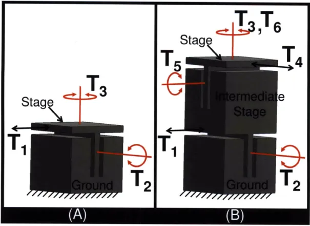
Consider the 3 DOF system that is constrained by the flexure blade in Figure 2.4A. The system's stage is permitted to move with a translation and two rotations as depicted by the three twists that are shown in the figure. If this parallel flexure module were stacked on top of itself as shown in Figure 2.4B, one might expect the new stage to possess 6 DOFs-3 from each module. Although the stage inherits the DOFs of both parallel modules as shown in Figure 2.4B, the stage only possesses 5 DOFs because the rotations labeled T3 and T6 are redundant meaning that both

parallel modules possess the same DOF. When a serial flexure system possesses one or more

redundant DOFs, the system is underconstrained. When the system's stage and ground are held

fixed, underconstrained systems possess one or more intermediate stages that are not fully constrained. Under such conditions these intermediate stages are free to move with the DOFs that are redundant. Consider, for example, holding the stage and ground of the serial flexure system from Figure 2.4B fixed. The intermediate stage labeled in the figure would remain free to rotate about the axis of the rotation labeled T3 and T6. It will later be demonstrated how

geometric shapes may be used in conjunction with the principles of this section to avoid or utilize underconstraint in the design process of serial flexure systems.

(34)

U

e,,Z~ol-7171/

Figure 2.4: 3 DOF parallel flexure system (A). 5 DOF stacked serial flexure system (B).

Advantages and challenges are associated with flexure systems that are underconstrained. Parallel modules stacked in series like those shown in Figure 1.2B and Figure 2.4B achieve a greater range of motion than the individual parallel modules alone. The reason for this increase in range is that the redundant motions of each module contribute to the full stroke of the final stage. A properly underconstrained system may, therefore, markedly increase a flexure's stroke to size ratio. Unfortunately, underconstrained flexure systems generally have poor dynamic characteristics. Reducing the mass of the intermediate stages and stiffening the flexible elements that connect them together helps mitigate this problem.

2.2.3 Intermediate Spaces

Consider the planar constraint space of the parallel flexure module from Figure 2.4A. This constraint space is shown with a different orientation in Figure 2.5A. Note that the constraint lines of the flexure blade shown in Figure 2.5B lay on the plane of the system's constraint space. The constraint space belongs to the first type in the 3 DOF column in Figure 2.2. The constraint

T5

T4

3 _eT

Stage

(35)

space's complementary freedom space, shown in Figure 2.5A, consists of all rotational lines that lie on the plane of the constraint space as well as a translation perpendicular to this plane. Notice from Figure 2.5B that the three DOF twists shown in Figure 2.4A belong to the freedom space of the system. If the parallel flexure module is stacked in series with itself as shown in Figure 2.5C, the resulting freedom space of the serial stage not only possess twists from the planar freedom spaces of each individual parallel flexure module, but it also possesses the twists that result from combining the twists of these spaces. The freedom space of the serial flexure system's stage, therefore, contains (i) every rotational line that lies on the planes that intersect the dotted line shown in Figure 2.5D and (ii) every translation that is perpendicular to the same line. Note that the two planar freedom spaces of the two individual parallel modules both lie within this freedom space. The two freedom spaces that combine to form the serial system's freedom space are called intermediate freedom spaces. These spaces each contain three independent twists that are labeled in Figure 2.5C. These twists may be combined to generate the other twists within each space. Together, however, the six twists combine to generate all the twists shown in the freedom space of Figure 2.5D. If Gaussian elimination were performed with these six twists, only five of them would be shown to be independent. It is not surprising therefore, that the freedom space shown in Figure 2.5D belongs to the first type in the 5 DOF column of the chart shown in Figure 2.2 because the system possesses only five DOFs.

T4T5,T6

5 DOFs

3

T1T

2

T2

3

Figure 2.5: 3 DOF Type 1 freedom and constraint spaces (A). Spaces imposed on the 3 DOF

parallel flexure module (B). Intermediate freedom spaces (C) sum together to produce the 5 DOF

freedom

space of the serial flexure system (D).

(36)

Intermediate freedom spaces always exist within a system's freedom space. The total number of independent twists from all of the intermediate freedom spaces combined must equal the number of DOFs within the desired system freedom space. If this condition is not satisfied, the intermediate freedom spaces of the stacked parallel flexure modules will not produce the correct DOFs.

Intermediate freedom spaces help designers identifying whether or not a serial flexure system is underconstrained. If the sum of the number of DOFs of each intermediate freedom space is more than the number of DOFs of the system's freedom space, the serial flexure system will be underconstrained and will possess redundant DOFs. Note that the serial flexure chain from Figure 2.5 is underconstrained because the sum of the number of DOFs from each intermediate freedom space is six, and six is greater than the number of DOFs of the system's freedom space (5 DOFs).

2.2.4 Kinematic Equivalence

The freedom and constraint spaces of the serial flexure chain from Figure 2.5D are shown as Type 1 in the 5 DOF column of the chart of Figure 2.2 and again in Figure 2.6A. Note that the freedom space not only contains rotation lines and translations, it also contains screws. The shapes that describe the locations and orientations of these screws are described in detail in Chapter 3. The constraint space of the system is a constraint line that is collinear with the line of intersection of the planes of rotation from the freedom space. Note that a single flexure wire constraint also possesses the same freedom and constraint spaces as shown in Figure 2.6B. A flexure wire is a long, slender flexible element. The flexure wire and the serial flexure chain from Figure 2.6C are said to be kinematically equivalent because they possess the same freedom space. The parallel and serial flexure systems shown in Figure 2.6D are also kinematically equivalent because the flexure wires of the parallel flexure system were replaced with the kinematically equivalent flexure chains of the serial flexure system. Although kinematically equivalent flexure elements may be substituted without changing a system's DOFs, the system's elastomechanics, dynamics, and manufacturability may be altered to satisfy desired design requirements.

(37)

Figure 2.6: 5 DOF Type 1 freedom and constraint space (A). Spaces imposed on the 5 DOF

wire flexure (B). Wire flexure and serial flexure chain are kinematically equivalent (C). Two kinematically equivalent flexure systems (D).

2.3 FACT Design Process

This section describes the 6 steps of the FACT design process shown in Figure 2.7 that is used to synthesize precision flexure systems. A lead screw flexure will be designed using FACT.

(38)

Figure 2.7: Steps of the FACT design process

Step (1): Identify Desired Motions

The designer must first recognize which DOFs the system should possess.

Step (2): Identify Freedom Space

The designer must then identify the freedom space that embodies the DOFs that were specified in Step (1). This freedom space will belong to the column from Figure 2.2 that pertains to the number of DOFs the system should possess. If the designer is not familiar enough with the spaces to recognize which space contains the desired DOFs, a computer code could be written using the materials from Appendix A and Hopkins [21] that identifies this freedom space from the appropriate column.

Step (3): Parallel or Serial?

The designer must then decide whether to synthesize a parallel or a serial flexure system. If the freedom space identified in Step (2) does not belong inside the parallel pyramid from Figure 2.2, then the designer must synthesize a serial flexure system to achieve the desired DOFs. If, however, the freedom space does belong inside the parallel pyramid, then parallel or serial concepts exist that achieve the desired DOFs. Designers are generally encouraged to first

(39)

attempt generating parallel concepts before generating serial concepts because parallel concepts

(i) do not suffer from stacked axis errors, (ii) are easier to design and fabricate, and (iii)

generally possess better dynamic characteristics than serial flexure systems.

Step (4): Choose Intermediate Freedom Spaces

If the designer chooses to synthesize a serial flexure system, intermediate freedom spaces must

be selected. The intermediate freedom spaces must exist in the chart of Figure 2.2 to the left of the column that contains the selected freedom space because the intermediate freedom space must exist within the freedom space. The intermediate freedom spaces must also belong within the parallel pyramid. If the designer has trouble recognizing feasible intermediate freedom spaces, a computer code could be written that identifies them. This code would rely on the materials from Appendix A and theory in Hopkins [21]. Designers may select any number of viable intermediate freedom spaces. An intermediate freedom spaces may be selected multiple times. The number of intermediate freedom spaces determines the number of rigid stages or conjugated elements the flexure system will possess. The fewer the stages, the less complex the design, the easier to fabricate and assemble, and the better will be the dynamic characteristics. Serial flexure systems require a minimum of two intermediate freedom spaces. Intermediate spaces that possess orthogonal features generally produce designs that are easily fabricated.

Step (5): Design Ground and Stage/s

The ground and rigid stages must then be designed. If the designer chose to synthesize a parallel flexure system, only one stage should be designed. If the designer chose to synthesize a serial flexure system, the number of stages should equal the number of intermediate freedom spaces that were selected from the previous step. The rigid stages should be far enough away from each other that they do not collide as they move.

Step (6): Select Constraints from Constraint Space/s

If the designer is synthesizing a parallel flexure system, he/she must select constraints from the

constraint space of the system's freedom space. These constraints must connect the ground to the rigid stage. If the designer is synthesizing a serial flexure system, constraints from the constraints space of the first intermediate freedom space must be selected such that they connect

Design of flexure-based motion stages for mechatronic systems via Freedom, Actuation and Constraint Topologies (FACT)

Design of Flexure-based Motion Stages for Mechatronic

Systems via Freedom, Actuation and Constraint Topologies

(FACT)

OFCHIVES

ARCHNVES

7)

i

upervisor

Design of Flexure-based Motion Stages for Mechatronic

Systems via Freedom, Actuation and Constraint Topologies

(FACT)

ABSTRACT

ACKNOWLEDGMENTS

TABLE OF CONTENTS

LIST OF FIGURES

LIST OF TABLES

CHAPTER 1:

Introduction

1.1 Research Objectives

1.1.1 Serial Flexure Synthesis

1.1.2 Optimal Actuator Placement

Error

Probe's

-.

Tip

A

1.2 Fundamental Principles

1.2.1 Modeling Motions via Screw Theory

AO

p

c

z

x

y

Rotation =0 Translation p=oo Screw p404

oo

1.2.2 Freedom Space

1.2.3 Modeling Flexible Constraints via Screw Theory

q

r

z

X

en

Pure Force q=0 Pure Force q=0

1.2.4 Constraint Space

[W]=[W,

1.2.5 Constraint and DOF Relationship

[<b].T=0,

[]=

(1.7)

1.2.6 Modeling Actuators via Screw Theory

1.2.7 Decomposing Wrench and Twist Vectors

q -

r

r,

1.3 Thesis Overview

CHAPTER 2:

Serial Flexure Synthesis

2.1 FACT Chart

2.2

Serial Synthesis Principles

2.2.1 Parallel and Serial Constraint Fundamentals

Disk of

Translations

2.2.2

Underconstraint

2.2.3 Intermediate Spaces

T5

T4

3

eT

Stage

T4T5,T6

5 DOFs

T1T

T2

freedom

2.2.4 Kinematic Equivalence

2.3 FACT Design Process

_A

_y

_{Pure Force q=0 Pure Force q=0}

_eT