Characterization of hot-carrier reliability in analog sub-circuit design

Characterization of Hot-Carrier Reliability in Analog

Sub-circuit Design

by

Huy X. P. Le

Submitted to the Department of Electrical Engineering and Computer Science

in partial fulfillment of the requirements for the degree of

Master of Engineering in Electrical Science and Engineering

at the

MASSACHUSETTS INSTITUTE OF TECHNOLOGY

May 1996

@ Huy X. P. Le, MCMXCVI. All rights reserved.

The author hereby grants to MIT permission to reproduce and distribute publicly

paper and electronic copies of this thesis document in whole or in part, and to grant

others the right to do so.

Author...

_{A uthor}

_...

..

_E1.ctrical"

_ý

_{... ..}

_77:ý...

Departm nt of Eldctrical Engineering and Computer Science

t

March 8, 1996

Certified by ...

....

". .

...

..

-(1

i

.. .. . .. . .. .. . .. .. . .. . .. .. . .. .

James E. Chung

Associate Professor

Thesis Supervisor

"b

Accepted by...

k

.

Frederic R.

Morgenthaler

"'hairman, Departmental Committee on Graduate Students

MASSACHUSETTS INSTI'U FE

OF TECHNOLOGY

JUN

I1

1996

Characterization of Hot-Carrier Reliability in Analog Sub-circuit Design

by

Huy X. P. Le

Submitted to the Department of Electrical Engineering and Computer Science on March 8, 1996, in partial fulfillment of the

requirements for the degree of

Master of Engineering in Electrical Science and Engineering

Abstract

The focus of hot-carrier reliability study in recent years has shifted from the modeling of the physical phenomenon at the device level toward understanding the relationship be-tween the AC degradation and its impact on circuit performance. However, most of the effort has been targeted at digital applications, and very limited work has been done on applications requiring analog functions. Increasingly, there is a need to address the issue of hot-carrier reliability in the area of analog circuit design since the traditional lifetime prediction methodology applicable for digital circuits is no longer valid for analog circuits where the devices are not always operated in saturation and key circuit performance pa-rameters depend on the matching properties of the devices, Leff, biasing conditions, and circuit topology.

Through simulation, this thesis systematically looks at the methodology of designing for hot-carrier reliability in analog circuits. By studying hierarchically the degradation of the circuit building blocks most utilized in an operational amplifier, we first examine the existing tools and methodology for hot-carrier degradation evaluation. In a larger context and framework of evaluating the reliability of analog-circuit designs, a set of systematic steps is then proposed to be carried out in modifying, improving , and developing new algorithms and design guidelines. The end goal is to get a better understanding and insight into the trade-offs of the different designs and reliability, and more fundamentally, what it means to have a 10%AgM, or O10%AVOFFSET at the circuit level.

Thesis Supervisor: James E. Chung Title: Associate Professor

Contents

1 Introduction

1.1 Hot-Carrier Effects & Degradation ... 1.2 Degradation Model ...

1.3 The Concept of Accelerated Stressing . . . . 1.4 Reliability Simulation Tools ...

1.5 Hot-carrier Degradation & Circuit Reliability . . . 1.6 Thesis Overview ...

2 Experimental Framework

2.1 Tool Calibration Issues ... 2.1.1 SPICE Model Fitting ...

2.1.2 Hot Carrier Degradation Model Parameters 2.2 Analog Design Space ...

2.2.1 Low Frequency Differential Pair . . . . 2.2.2 High Frequency Differential Pair . . . . 2.2.3 Mixed Frequency Differential Pair . . . . . 2.2.4 Simple Current Mirror ...

2.2.5 Cascode Current Mirror ... 2.2.6 Wilson Current Mirror ... 2.2.7 Bias-Voltage Generator ... 2.2.8 Common-Source Amplifier ... 2.2.9 Source Follower ... 2.2.10 Design Verification ... 6 . . . . 6 . . . . 9 . . . . 11 . . . . 11 . . . . 12 . . . . 13 15 . . . . 15 . . . . 15 . . . . . 17 . . . . 18 . . . . . 20 . . . . . 22 . . . . . 22 . . . . 23 . . . . 24 . . . . 24 . . . . 25 . . . . 26 . . . . 26 . . . . 27

3 Simulation Result & Discussion

29

3.1 NMOS Device Simulation ... 29 3.2 PMOS Device Simulation ... 31 3.3 Differential Pair Simulation ... 32

4 Conclusion

35

A BERT: Limitations of HCI Reliability Simulation

37

B SPICE & BERT Simulation Input Files

42

B.1 BERT Command File ... 42 B.2 SPICE Netlist for MOSFET Simulation ... 43 B.3 Netlist for Differential Pair Simulation ... 43

List of Figures

1-1 MINIMOS simulation of lateral electric field [1] . . . . . 7

1-2 Cross section of an NMOSFET showing hot-carrier effects [2] . . . . . 8

2-1 ID-VD parameter extraction of a fresh device using BSIM2 model . . . . . 16

2-2 Rout-VD fitting of an degraded device using BSIM2 model . . . . . 17

2-3 Hot-Carrier parameters fitting for use in this thesis . . . . . 18

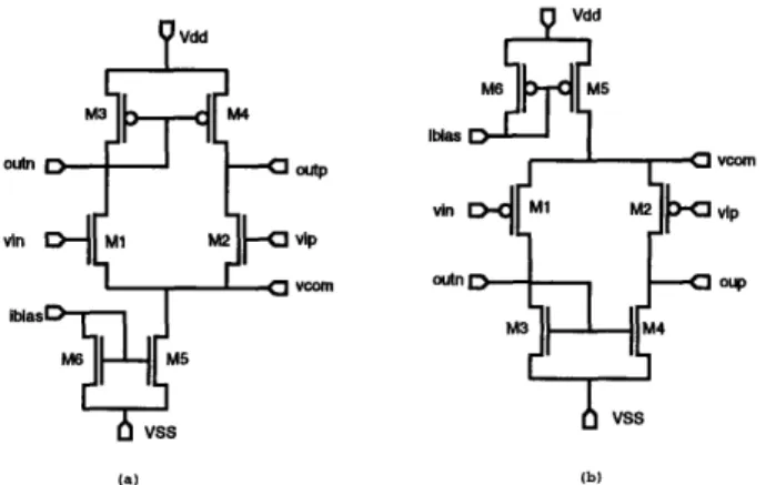
2-4 Schematic of differential pair with emphasis on accessibility of the internal nodes . . . 21

2-5 Schematic of differential pair with emphasis on high frequency testing. . . . 22

2-6 Schematic of differential pair compromising between accessibility and high frequency testing ... 23

2-7 Schematic of simple current mirror . . . . 24

2-8 Schematic of cascode current mirror . . . . . 24

2-9 Schematic of Wilson current mirror . . . . . 25

2-10 Schematic of bias voltage generator . . . . . 26

2-11 Schematic of common source amplifier . . . . . 26

2-12 Circuit schematics for the source follower . . . . . 27

3-1 Simulated degradation vs. raw degradation for a single NMOSFET... .. 30

3-2 Experimental fresh and degraded IV for both N and PMOSFETs [10] .. . 32

3-3 Simulation of the fresh and degraded Bode plots for a differential pair . . . 33

3-4 Experimental data of the differential pair stressing [22] . . . . . 34

A-1 Inner working of BERT ... 38

A-2 Linear and quadratic dependency of MUo and U0lo in linear scale . . . . . 40

C-1 Layout of the test circuit of the low-frequency differential pair (Figure 2-4). 46 C-2 Layout of the test circuit of the high-frequency differential pair (Figure 2-5). 47 C-3 Layout of the test circuit of the mixed-frequency differential pair (Figure 2-6). 48

C-4 Layout of the test circuit of the simple current mirror (Figure 2-7) . . . . . 49

C-5 Layout of the test circuit of the cascode current mirror (Figure 2-8)... .. 49

C-6 Layout of the test circuit of the Wilson current mirror (Figure 2-9)... .. 50

C-7 Layout of the test circuit of the bias-voltage generator (Figure 2-10)... . 50

C-8 Layout of the test circuit of the common-source amplifier (Figure 2-11). . . 51

List of Tables

Chapter 1

Introduction

With a combination of technology scaling, architectural re-design, and creative program-ming, the speed and density of modern VLSI systems has increased by several orders of magnitude. One of the goals of technology scaling is to try to keep the vertical and lateral electric fields constant in a device while continually reducing the device dimensions. If these two scaling constants are severely mismatched, the device performance will degrade, and consequently fail. Such an example is when the device channel length is scaled down from 1 - 2 pm into the deep submicron regime (around a one order of magnitude reduction) while the supply voltage is merely scaled down by a factor of 2 - 3. The resulting high-lateral electric field causes the mobile minority-carriers in the inversion layer to accelerate and reach velocity saturation. Such highly energized carriers-also known as hot carriers-can cause harmful and catastrophic failures to the device.

1.1

Hot-Carrier Effects & Degradation

If device dimensions are scaled down while the supply voltage remains constant (or is not reduced as rapidly as the device dimensions), the high lateral electric field generated near the drain-end region causes the mobile carriers to reach velocity saturation. This can be seen in Figure 1-1 where the 2-D simulator MINIMOS was used to simulate the lateral electric field along the channel of an NMOS device [1]. This exponential-like dependence of

D A %--_C 0 0 ..J

Figure 1-1: MINIMOS simulation of lateral electric field [1]. the electric field in the pinch-off region can be estimated from [3]:

VDS - VDsat

Emax

=1

1 _(1.1)

0.22 (tox) / (xj )

where tox is the gate oxide, and xj is the source/drain junction depth. Increasing Emax with decreasing device dimensions causes the mobile minority-carriers to gain kinetic energy and become hot.

A hot-carrier, while traversing the channel at maximum velocity, can cause impact ionization by colliding with the silicon lattice near the drain end, generating an electron-hole pair. This electron-electron-hole pair creation is only one manifestation of the high lateral electric field near the drain end of the device. As shown in figure 1-2, the peak Emax field can also affect devices in the following ways [2]:

* With sufficient energy, the initial electron-hole pair can create another electron-hole pair, and another, and another-leading to avalanche breakdown of the device (process 2 in Figure 1-2).

* In an NMOS transistor, the electrons created by the avalanche process are collected by the drain, and the holes diffuses to the substrate-constituting substrate current (process 3 in Figure 1-2). Due to high substrate resistance (10 ~- 1000 Q), the flow of substrate current can also raise the substrate potential and forward-bias parasitic p-n

Figure 1-2: Cross section of an NMOSFET showing hot-carrier effects [2].

junctions causing the circuit to latch-up (processes 4 and 5 in Figure 1-2).

* If the electrons from the electron-hole pair creation gain sufficient energy to surmount the Si - SiO2 potential barrier (-, 3.1eV), they can be injected into the gate oxide

to create an oxide trap or be trapped by an existing trap, giving rise to a shift in threshold voltage AVT (process 1 in Figure 1-2), as can be seen through [4]:

VT =

+ 2M

+ Qms b Qss (1.2)

Cýox

-

Cox

where 45m, is the metal-silicon work-function, 4 f is the Fermi potential, Qb is the

total charge in the inverted channel,

Q,s

is the total interface/oxide traps in the gate oxide, and Cox is the gate oxide.

* The highly energized mobile carriers can also break a silicon bond at the Si - SiO₂

interface to create an interface trap, resulting in decreased carrier mobility (AP). Hot-carrier degradation is not a catastrophic problem in the sense that the circuit does not fail suddenly. Rather, the device performance degrades gradually through the slow increase in threshold voltage VT and/or the decrease in mobility A. As a consequence, circuit performance degrades because the small signal parameters gin, 9ds, and IDsat are functions of VT and A.

The high value of Emax near the drain end arises partly due to the abrupt junction between the drain and the channel, and partly due to the high drain voltage Vds. To reduce this Emax, one can reduce the power supply voltage, or alternatively, introduce a graded doping profile junction so that the junction can absorb some of the voltage drop when

Vds > Vdsat. Such drain-engineering techniques are often used to fabricate double-diffused

drains (DDD) and lightly-doped drains (LDD) devices, making them more resistive to hot-carrier degradation. When this is done, a typical reduction of 30 - 40% of lateral Emax is observed which consequently reduces the the effects of hot-carrier degradation by orders of

magnitude'.

Although DDD and LDD structures have been shown to improve hot-carrier reliability, they posses drawbacks due to the increase in required process technology, and the resulting reduction in device performance. Because the source and drain have lower doping concen-trations for DDD and LDD devices, there is an increase in series resistance Rd and Rs which lowers the effective Vd, of the device. This results in a lower current driving capability of the device.

1.2

Degradation Model

Among the different hot-carrier effects described in 1.1, interface-state generation has been found to cause significant long-term degradation in MOSFETs. To quantify the amount of degradation experienced by a device, a physical model was developed based on the lucky electron concept [6]:

ANit oc

exp(-

T

(1.3)

where the exponential term exp(- i ) describes the probability an electron having suffi-cient energy to create an interface state with Oit being the critical energy needed to create an interface state, and qAEm being the kinetic energy gained by an electron while traveling along the channel. n simply describes the dynamics of ANit generation (whether interface state generation is diffusion limited or reaction limited). To check for device degradation easily, substrate current has been proposed as a degradation monitor since it has the same

functional dependence on the lateral electric field as interface state generation2 [6]:

Isub

-= -EmlcIdexp (-i

) (1.4)

In terms of I-V characteristics of the device, interface state generation results in a shift of the threshold voltage AVt, shift in the subthreshold current swing AS, and reduction in the transconductance in the linear and/or saturation region Agm. Using a simple gradual-channel approximation, a linear relationship was derived between the threshold voltage shift (AVT), relative transconductance reduction (Agm), relative mobility degradation (AM), and the number of interface states generated (ANit) [5]:

(

dDL -qL

AVT

o

WCo.

VD

+

)

it

(1.5)

•Ni - _GmGm

_(1.6)

OAGm

POa

_(1.7)

// -"1+a Nit

As can be seen, Equations 1.3 and 1.4 are both related to one another through the maximum electric field Emax in the pinch-off region (Equation 1.1) and provide a link between the electrical characteristics of a degraded device and its physical damage (Equations 1.5, 1.6, and 1.7). Details of this particular derivation and the detailed description of the constants can be found elsewhere [5].

By generalizing the degradation of transconductance, drain current, or threshold voltage as AD, we can model the hot-carrier degradation as [6]:

AD = (Age)n _(1.8) where Age(t) = I t DC condition (1.9) HW Id, I

Age(t)

=

N

-u

km

dt

AC condition

(1.10)

Jo

HW [Id,

The constant m-sometimes referred to as the voltage acceleration factor-is another way

2

one can write the term - i in Equation 1.3. The larger the m value (typically from

qAEEm

3 , 8), the harder it is for a hot-carrier to generate an interface state. The constant n, also referred to as the degradation rate coefficient, normally ranges from 0.5 , 1 [6]. H is simply a technology-dependent fitting parameters.

The age parameter describes how much stress a device experiences and determines the number of interface states (ANit) generated over time, for a given Ids, and Isub operating condition. The degradation AD is a power-law function of the age, and, for a given tech-nology, the graph of AD vs. age should fall on a universal curve for a wide range of possible channel lengths and device operating conditions.

1.3

The Concept of Accelerated Stressing

Since device parameter degradation can be calculated by the normalized value Age, one can get the same age of a device by:

* Operating the device at operational conditions at low VDS and VGS, and hence low

IDS and Isub, for a long time.

* Stressing the device at accelerated stress conditions at higher VDS, and hence higher

Isub, for a shorter period of time.

Because operating voltages VDS, VGS, and time are all related through equations 1.9 and 1.103, one can evaluate the hot-carrier reliability of a device by doing accelerated stress-ing experiments. This is desirable because evaluatstress-ing hot-carrier reliability at operational conditions would take a very long time. Typically, one would stress the device with a high

VDS to near the breakdown region in order to get a noticeable amount of degradation in a shorter time frame. One can then extrapolate back from the accelerated stress condition to the normal operating condition to predict the degradation of the device4

1.4

Reliability Simulation Tools

Through accurate modeling of the hot-carrier degradation mechanisms and basic under-standing of how a device ages, several hot-carrier reliability simulators have been developed.

3

A certain bias VDS and VGs will give rise to a fixed IDS and Is'aub.

4

One such example is the BERT tool [7], where all the major degradation mechanisms-oxide integrity, electromigration, and hot-carrier degradation-are modeled. Other hot-carrier circuit reliability simulation tools include HOTRON [8], and RELY [9].

The reliability tools BERT, RELY, and HOTRON are all built around some form of a transistor-level circuit simulator such as SPICE or HSPICE. The circuit simulation pro-grams provide information about the device terminal voltages and currents. The reliability simulation programs then use this information to estimate the dynamic stress condition, and consequently, the aging of each transistor in the given time interval. By doing a ta-ble look-up of each transistor's calculated age, a set of aged SPICE device parameters are extrapolated for each device in order to simulate aged circuit behavior. Circuit perfor-mance analysis can then be done to predict the impact of hot-carrier degradation on such parameters as switching frequency, low frequency gain, fT, and phase margin.

1.5

Hot-carrier Degradation & Circuit Reliability

To quantify the gradual nature of hot-carrier degradation in a circuit environment, a simple-minded approach would be to set a threshold limit for all device parameter variation and to declare a failure if the variation of that device's parameter exceeded the set threshold limit. This simplistic definition of failure has drawbacks impacting the general circuit performance. For example, if a device is not in a critical path, a larger parameter variation may be tolerable. However, if a transistor is in a critical path, a slight change in parameter value may have a large impact on the circuit performance. Therefore, the correct definition for circuit failure must incorporate both an understanding of device-level degradation mechanisms as well as an understanding of the impact of device degradation on circuit performance.

Work in recent years has shifted focus from trying to understand and model device-level degradation to understanding its impact on circuit performance. While some work focused on the degradation of the frequency in a ring oscillator (or Tpd of an inverter) [10, 11, 12],

other studies have focused on the effects of hot-carrier degradation in SRAM and DRAM performance [13, 14, 15]. With greater work and effort being spent in assessing digital-circuit reliability with respect to hot-carrier degradation, it is only worthwhile that some attention be focused on analog circuit-reliability.

and analog circuits onto the same chip. Since the world is analog in nature, this not only aids digital circuits interfacing with the physical world, but also helps in improving their computational performance.

Unfortunately, the existing circuit simulation models for digital ICs are not compatible with analog-circuit simulation because:

* An incorrectly modeled slope in the saturation ID - VG characteristics is of no conse-quence in most digital design. In analog design, however, it can mean an extremely inaccurate prediction of amplifier voltage gain.

* A small variation in the shape of the IV characteristics could make a big difference in the circuit sensitivity analysis.

Since the design and analysis of analog integrated circuits involves more than just a simple DC point evaluation, we need to re-examine and modify (if necessary) existing simulation models so that these models are more robust [16]. Furthermore, the most popular metrics for determining the accuracy of device models, such as RMS error of Id current, are adequate for evaluating models for digital-circuit design. However, if these same metrics were to apply to analog device models, one would get a very different outcome, because in analog-circuits, the important device model parameters are the small signal gm and gds, as opposed to the traditional IDsat which is important for digital circuits.

1.6

Thesis Overview

This thesis addresses the issue of hot-carrier reliability in analog circuit design based on the assumption that the existing degradation models and reliability simulators are adequate and can predict performance accurately (even for large and complex circuits). Instead of studying reliability for analog circuits in general, this study focuses particularly on the design of a differential amplifier and its subcircuit building blocks. By studying the problem hierarchically and systematically, we can get a better understanding into the trade-offs between the different circuit designs and reliability. We chose to focus on the class of amplifiers because of its frequent use in microprocessor as well as application specific ICs such as DSP chips.

and simulation of reliability in digital and analog integrated circuits. Chapter 2 shows the design issues involved for the particular subcircuit designs. It also explains how the circuit-simulation and reliability circuit-simulation tools are calibrated to a given technology. In Chapter 3, simulation results are presented, and discrepancies between preliminary experimental work and the simulation results will be discussed. Chapter 4 will conclude with some discussion on the ongoing efforts to verify the results from the simulations with real experimental data.

Chapter 2

Experimental Framework

2.1

Tool Calibration Issues

Several degradation models have been proposed to explain hot-carrier degradation and have been implemented in computer simulation programs. These programs can evaluate the effects of hot-carrier degradation on circuit performance quite effectively. However, ap-propriate procedures to calibrate these tools to a particular process have only been recently addressed as critical for the accurate prediction of lifetime [17]. Without careful calibration, these simulation tools would not be very accurate, thus limiting their overall impact and usefulness. Moreover, a typical reliability degradation simulation often relies on the volt-age waveform of only the first few cycles of circuit operation (- 10- 9 seconds) to compute the degradation out to 10 years (_ 10+8 seconds). This computation would result in an extrapolation of more than 10+17 cycles of simulation, requiring a high degree of accuracy in the simulation parameters (both for the degraded SPICE model parameters as well as the hot-carrier degradation parameters m, n, and H.

2.1.1

SPICE Model Fitting

Since hot-carrier degradation typically alters device performance by only a few percent during typical stress measurements, SPICE parameter extraction and optimization tools cannot afford to be more than a few percent off in RMS error. If the SPICE parameter extraction tool has more RMS error than the degradation itself, one may even not be able to distinguish between the fresh SPICE parameters and the degraded ones. Therefore, high

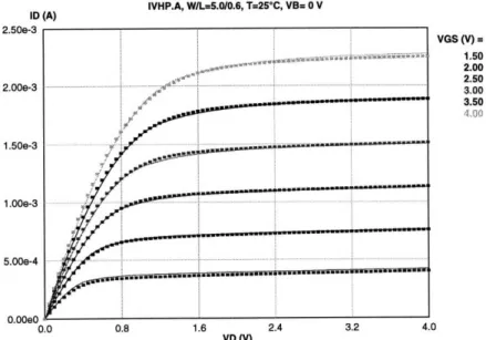
2.50e-3 2.00e-3 1.50e-3 1.00e-3 5.00e-4 0.00A0 VI HP.A WIL=5.0f0. , VB= 0 V ID (A) 0.0~e 1.6 2.4 3.2 4.0 VGS (V) = 1.50 2.00 2.50 3.00 3.50 VD (V)

Figure 2-1: ID-VD parameter extraction of a fresh device using BSIM2 model.

performance extraction and optimizing tools must be used. Furthermore, the MOSFET models available for analog design and simulation may have addition problems that are not significant for a digital design. For example, the same specific models in various simulators may behave differently from one another due to differences in their particular implementa-tions [16]. Poor fitting of a SPICE model could also be the result of using too simple of a model, or simply due to poor parameter extraction. For the above reasons, all SPICE simulations in this study use the BSIM2 SPICE model (model 39) to ensure proper behavior

of the model in all biasing ranges.

Typical parameter extraction and SPICE fitting results for the BSIM2 model are shown in Figures 2-1 and 2-2. Only a few example of parameter fittings are shown here, and even with one the most advanced MOSFET models (BSIM2), the fit of the drain current and output resistance is still poor at the 'knee' region where the transistor changes from the linear to the saturation region. Recent improvements in the MOSFET model BSIM3 greatly rectify this problem, but the model has yet be implemented in the currently-available design

tools.

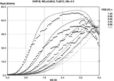
Notice that the ID-VD curves show a much better fitting than Ro-VD curves. In Figure 2-1, we were able to achieve less than 2% RMS error, but with Figure 2-2, the best we could do was a 40% RMS error. This is an illustration of how models and tools are tradi-tionally optimized for digital-circuit simulation rather than analog-circuit modeling since in digital circuits, one is only concerned with saturation current drive rather than small-signal

VI HP B WIL=5.01 V Rout (Kohm) 80.0 64.0 48.0 32.0 16.0 A0n VGS (V) = 1.50 2.00 2.50 3100 3.50 0.0 0.8 1.6 2.4 3.2 4.0 VD (V)

Figure 2-2: Rout-VD fitting of an degraded device using BSIM2 model.

parameters such as ro for analog circuits.

2.1.2

Hot Carrier Degradation Model Parameters

Almost all AC hot-carrier degradation models and reliability simulation tools are based on the general concept of hot-carrier 'AGE' as described in the previous chapter. This abstract quantity, as defined by Equation 1.9, has an inversely-proportional relationship to H and an exponential relationship to m; any small error in extracting these quantities could result in large error in predicting degradation. Furthermore, the stress-bias dependence of the hot-carrier degradation rate n has been shown to cause poor lifetime prediction if not properly taken into account [18].

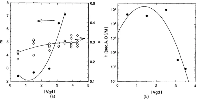
As mention previously and also noted in Appendix A, reliability simulation often requires large extrapolations based a few initial data points using model fitting parameters that can vary by orders of magnitude (Figure 2-3-b). In this study, to improve model accuracy, a large number of devices were stressed, from which degradation model parameters were extracted, in order to account for any statistical and experimental variations. The hot-carrier degradation parameters m, n, and H for NMOSFETs have been extracted based on a 10 percent linear-current degradation lifetime definition, and modeled as a quadratic function of Vgd. The model fitting of these parameters is shown in Figure 2-3, and the

106 0.4 105 S104 0.3 0 (D 103 0.2 102 0 1 1n1 0 1 2 3 4 5 0 1 2 3 4 I Vgd I I Vgd I (a) (b)

Figure 2-3: Hot-Carrier parameters fitting for use in this thesis. quadratic function modeling these parameters was found to be:

m = 3.376 - 2.233 Vgd + 0.96 V2d (2.1)

n = 0.230 - 0.0424 Vgd - 0.0044 V2d (2.2)

log H = 4.346 + 2.743 Vgd - 0.998 V2 (2.3)

2.2

Analog Design Space

The performance of digital circuits may not depend as critically as analog circuits on such circuit parameters as biasing conditions, matching properties of the devices, or on device parameters such as and threshold voltage shift (AVt). As can be seen in the following two equations, whereas the digital circuit parameter -rpd of an inverter is quite insensitive to device variation, the transconductance Gm of a differential pair can vary significantly with device variation [4, 19]: Tpd o 1 (2.4) Sc (Vdd -t) 2 Gm = gm OC (V98- Vt) (2.5) 7 6 E 5 4 3 2

This can be seen more clearly if one differentiate these two equations for the circuit param-eters Tpd and Gm with respect to the device parameter Vt and evaluating them at Vt0:

6

(Tpd 2

SVt )3 (2.6)

cGm -1 _(2.7)

The denominator of Equation 2.6 will always be greater than one, hence the sensitivity of Tpd (Equation 2.6) with respect to Vt would always be smaller than the sensitivity of

Gm (Equation 2.7) with respect to Vt. Furthermore, the sensitivity of an analog circuit parameters depends a lot on perturbations in the SPICE parameters as well as the particular circuit operating environment. Thus, the circuits in this thesis have been designed to span many dimensions to study the different dependencies and sensitivities of circuit performance. Ranging from basic biasing circuits to basic gain stages, the circuits designed in this thesis serve as the building blocks of more complex analog functions and subsystems. Al-though implementations may vary from design to design, the circuits presented here show the simplest way one could implement the given function. Beginning with analog subcircuit blocks such as differential pairs, current mirrors, bias voltage generators, gain stages, and output stages, models and understanding will build upon the analysis and experimental data gathered from stressing each of these subcircuit blocks. Instead of the traditional device lifetime plots, we will concentrate on a set of analog hot-carrier design curves based on the simulation of the 'composite' amplifiers using simulation tools such as HSPICE and BERT.

One may question the methodology we take in evaluating the degradation and reliability of the subcircuits since, after all, the device degradation and its interaction among the subcircuits may not be as valid and well behaved as we have assumed it to be. Whether it

is valid to 'break up' the circuits in this manner and model degradation as a black box with terminals that can interact across each of the subcircuits remains unclear. However, from our previous experience, one can model the performance behavior of an operational amplifier this way, and since hot-carrier degradation is directly related to circuit performance and behavior, the assumption that degradation can be modeled as a series of connected black boxes is a good one. The validity of this assumption will be verified with experimental data. These circuits were designed to maximize the VDS on each transistor-and to enhance

II

M1

M2

M3

M4

M5

M6

M7

M8

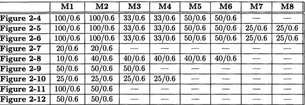
Figure 2-4 100/0.6 100/0.6 33/0.6 33/0.6 50/0.6 50/0.6 - -Figure 2-5 100/0.6 100/0.6 33/0.6 33/0.6 50/0.6 50/0.6 25/0.6 25/0.6 Figure 2-6 100/0.6 100/0.6 33/0.6 33/0.6 50/0.6 50/0.6 25/0.6 25/0.6 Figure 2-7 20/0.6 20/0.6 - - - - - -Figure 2-8 10/0.6 40/0.6 40/0.6 40/0.6 40/0.6 40/0.6 - -Figure 2-9 50/0.6 50/0.6 50/0.6 - - - - -Figure 2-10 25/0.6 25/0.6 25/0.6 25/0.6 - - - -Figure 2-11 100/0.6 50/0.6 - - - - - -Figure 2-12 50/0.6 50/0.6 - - - - -

-Table 2.1: W/L of transistors used in figure 2-4 to 2-12 (in micron).

hot-carrier degradation-especially those devices that are 'stacked' between power and ground rails. Unlike digital circuits where a typical transistor sees a full Vdd across the drain and source terminals, a transistor in an analog circuit will only see a fraction of Vdd in a typical operating condition. Therefore, all transistors have minimum feature size to accelerate the hot carrier degradation, with the exception of a few channel-length variations of some circuits to verify the channel length dependence of hot-carrier degradation in analog circuits.

The dimensions of the transistors are listed in Table 2.11. A variant of these subcircuits are the sister-class of circuits where PMOS and NMOS devices substitute for one another. The following figures capture most the ideas of this project, and provide a brief explanation for what we would hope to see from each subcircuit block. In each figure, the NMOS flavor is shown in (a), and its corresponding PMOS sister is shown in (b).

2.2.1

Low Frequency Differential Pair

This represent a broad class of circuits whose basic function is to amplify the difference between the two input signals. The bias level and gain of such a stage depend on the

symmetry between the two branches of the circuit making it an ideal gain block in most integrated circuits. The differential pair is attractive for its ability to be cascaded without requiring either DC level shifters or coupling capacitors. A typical configuration may have a passive (resistive) load or an active (current mirror) load. The active-load differential pair can provide higher gain because the output impedance of a current source is (theoretically)

1

Variant of figure 2-4 includes fixing the PMOSFETS and varying NMOSFETS channel length to 0.8 and 1.0 pr, and fixing the NMOSFETS and varying the PMOSFETS channel length to 0.8 and 1.0 pm

VroM

VIp

oup

u voo

(a) (b)

Figure 2-4: Schematic of differential pair with emphasis on accessibility of the internal nodes.

infinite. Normally, a differential pair would have a differential output where the signal voltage is taken between the two output nodes. Shown in Figure 2-4 is the differential to single-ended conversion implementation of the differential pair circuit.

Figure 2-4 shows the schematic of a simple differential pair where each of the individual transistor within the subcircuit can be probed and monitored for degradation, or individu-ally be stressed in order to study how the asymmetrical degradation of the devices affects the matching properties of the differential input pair. Because of the probing pads present at the AC nodes outp, outn, and vcom, the bandwidth performance of this circuit is expect-edly poor and simulated to be no more then 10MHz. If we take the output at node outp and the input at node vin, the gain of the differential pair can be calculated as:

AV

_ Voutp = 9m2 X

gds4

(2.8)

vvin

where gm2 and gds4 can be found by differentiating

Ids

=

Cox

2

(V

- V)2

(2.9)

and evaluating it at the appropriate bias condition. Looking at this circuit by grounding

vip, the input vin to output outp can be seen as a common gate amplifier. The DC node

ibias.-Iblas

(a) (b)

Figure 2-5: Schematic of differential pair with emphasis on high frequency testing.

2.2.2 High Frequency Differential Pair

One limitation of the low-frequency differential pair is the large output load capacitance at node outp that prevents the signal from achieving high bandwidth. By incorporating the source follower, we can achieve a higher bandwidth without sacrificing gain as shown in Figure 2-5. With this configuration, we hope to study hot carrier effects at a higher frequency at the cost of losing the capability of internal probing to characterize the individ-ual transistors. Figure 2-5 shows the schematic of a simple differential pair with a source follower simulating the realistic operating condition of a typical amplifier. Because there is minimal loading capacitance in the internal nodes, the frequency response is expected to be superior to that of Figure 2-4. However, we cannnot monitor/stress the individual transistors from within the subcircuits.

From this circuit we can only measure how the frequency response behaves as the sub-circuit is stressed over time. By cascading the source follower with the differential pair, we have effectively trade the increase in bandwidth of the circuit for the effective gain, since the gain of a source follower is not quite unity 2

2.2.3

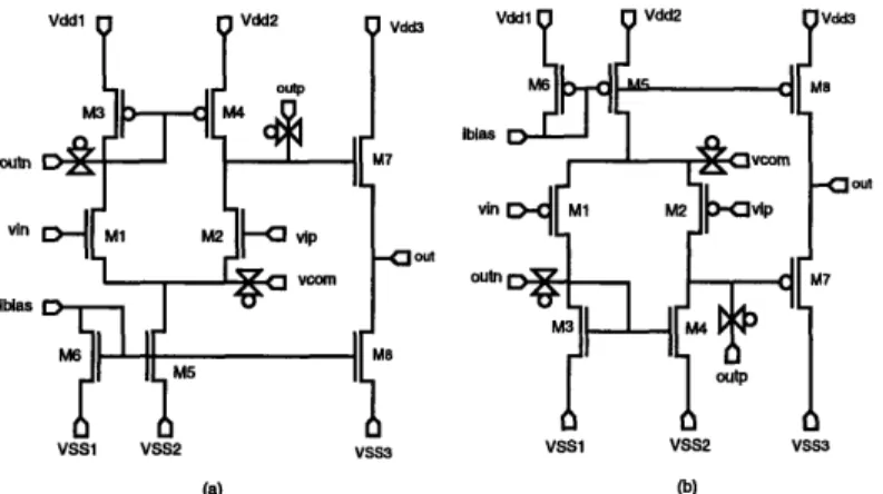
Mixed Frequency Differential Pair

The low-frequency and high-frequency differential pairs present the two extreme cases of testability in our designs. On the one hand, the design in Figure 2-4 provides for accessibility to the internal nodes of the circuits at the expense of frequency limitation. On the other hand, the design of Figure 2-5 allows the testing frequency to go higher but at the cost of internal-node probing and monitoring. A good compromise between these two designs is

2

ouin

vin

Iblas

VSS1 VSS2 VSS3

(a) (b)

Figure 2-6: Schematic of differential pair compromising between accessibility and high frequency testing.

shown in Figure 2-6 where CMOS pass-gate transistors were added to the high-frequency differential pair. With this design, one still can individually monitor each device in the subcircuit as it degrades, but the complexity of the test setup has increased by one order of magnitude. The presence of parasitic junction-capacitances of the pass-gate transistors is minimal as compared to the large gate-capacitances of each of the transistors, thus not limiting the circuit bandwidth significantly.

2.2.4 Simple Current Mirror

In order for the differential pairs to work properly, appropriate current biasing conditions must be established to keep the input transistor pair ml and m2 in saturation. Another way to look at the basic differential-pair is a pair of source-coupled NMOS transistors in cascode with 2 current sources (one PMOS type, and one NMOS type). The goal of a current mirror is to establish a DC node that is capable of sourcing or sinking current, and with a high small-signal impedance to ground. One simple-minded way to do this is shown in Figure 2-7. Output resistance in this configuration is limited by the channel-length modulation coefficient, and in sub-micron dimensions, this coefficient can be quite large.

The purpose of this subcircuit is to study how the mismatch in current mirrors due to hot-carrier degradation can affect the circuit-level performance. The symmetry of the device and design layout would be reduced when one of the transistor's Vt is shifted due to hot-carrier degradation. We want to explore how degradation tracks the current matching behavior of the circuit. For completeness, we have included the PMOS class of the current mirror, while in practice, the NMOS current mirror alone is sufficient.

ibias vout Vdd

ibias Vout

(b)

Figure 2-7: Schematic of simple current mirror.

Vdd vi vout Vdd

(a) (b)

Figure 2-8: Schematic of cascode current mirror.

2.2.5 Cascode Current Mirror

A cascode configuration, such as one shown in Figure 2-8, can achieve a much higher output resistance. Since this is a desirable characteristics in a current source, a cascode current mirror is often used in circuits where the power supply is greater than a few volts. In low power supply design, it is more difficult to use a cascode circuit such as the one shown here since the 'head-room', or swing voltage at the output node, is limited as the transistors are stacked up. In the cascode design, a minimum voltage must be maintained at the output terminal to keep transistors M5 and M6 in saturation. Hot-carrier degradation may cause the node voltages to drift, thus driving some of the transistors out of saturation and into linear region-reducing the effectiveness of the cascode configuration.

2.2.6 Wilson Current Mirror

Another method to improve the output resistance of a current source is to use negative feedback in the manner known as the Wilson current mirror as shown in Figure 2-9. By employing negative feedback through transistor M2, the effective output resistance seen at

vout ibias

(b)

Figure 2-9: Schematic of Wilson current mirror.

vout is found to be [4]:

rout (2 +

gm3

rol)

ro

3

(2.10)

The feedback action works as follow. As lout decreases slightly, node v1 decreases, and in order to maintain the fixed Ibias, the Vd, of M1 would have to increase. As a result, the effective Vg, of M3 is increased making Iout larger. The Wilson current mirror also suffers from similar problems as other current mirrors, and any threshold voltage deviation (due to hot-carrier degradation) will lead to drain-current mismatch.

2.2.7 Bias-Voltage Generator

In a variety of circuit applications, it is necessary to establish a low-impedance point within the circuit which can serve as an internal voltage supply. Ideally such a voltage reference point is required to have both a very low AC impedance, and a very stable DC voltage level which is insensitive to power supply and temperature variations. Such circuits are known as voltage sources or references. A simple way of implementing a bias-voltage reference is to cascode the diode-connected transistors between the power and ground rails as shown in Figure 2-10. The reference voltage generated at nodes v1, v2, and v3 can be controlled by

varying the device dimensions (L

,

()2,

and

(L).

Many circuits have been proposed to generate DC voltages that are independent from power supply voltage or temperature. However complex these circuits may be, hot-carrier

Vdd VSS M1 M4 V1 V3 V2 V2 M2M2 M3 V2 J 4V2 M3 M2 V3 V1 M4 M1 I VSS _Vdd (a) (b)

Figure 2-10: Schematic of bias voltage generator.

Vdd

VIp _M1

Vout Vin H M2

VVSS

Figure 2-11: Schematic of common source amplifier.

2.2.8

Common-Source Amplifier

The common-source amplifier is commonly used in operational amplifiers for second-stage gain. As an amplifier in itself, hot-carrier degradation of the common source amplifier may not be as interesting as if it was used for second-stage gain. In a Miller-compensated configuration, the common-source amplifier is directly in the feedback path, and, depending on the design, fT may be a function of g9m2 where 9m2 is the second stage gain. Hot-carrier degradation resulting in a reduction in g9m2 may lead to circuit instabilities when fT shifts or the phase margin decreases. With this configuration (shown in Figure 2-11), one can achieve very high gain with low biasing current as a single gain stage since it is a common source amplifier with an active (current source) load .

2.2.9

Source Follower

Sometimes known as a level shifter, this class of subcircuit insures the DC level of one part of the circuit is compatible with another part of the circuit. Such a circuit is needed, for example, when common-source gain stages are cascaded, and the output DC level of one

3

Vdd Vdd Vin -dM1 Vb DAM, Vout _.. Vout Vb D-] M2 Vip DA M2 u vss rlvss (a) (b)

Figure 2-12: Circuit schematics for the source follower.

stage is higher than the input DC level of the next stage. Due to its high input-impedance and low output-impedance nature, this kind of circuit is often used as a unilateral buffer between successive gain stages to prevent loading. It is also sometimes used at the output stage where small output impedance is required. The schematics are shown in Figure 2-12. When used as an output stage, it is the simplest technique to achieve large output current swing, low output impedance, low signal distortion, and excellent frequency response. The gain of this stage is approximately [19]:

A - v _Vin - _gdsl+gds2 gout _{9m +} (2.11)

9mb1

where, in the limit of gmi

>

9mbl or 1 the gain approaches unity. 9ds1 +Yds2 '

Depending where the input signal is applied and where the output signal is taken, Figure 2-12 can also be configured as a common-gate amplifier. For example, if the input signal is applied at vb, and the output is taken at vdd, with vin biased at a DC voltage, the amplifier could be used as a current buffer, or a very high gain voltage amplifier without sacrificing bandwidth due to the missing coupling capacitance from input to output.

2.2.10

Design Verification

Using the data to be gathered from each subcircuit blocks, a 'composite' operational ampli-fier will be simulated using circuit simulators such as HSPICE and reliability tools such as BERT. By doing so we hope to gain further insight into the relationship between circuit relia-bility and performance in analog circuit design. Upon the completion of this study, it may be worthwhile to re-assemble these subcircuits into a complete Miller-compensated operational-amplifier and verify the degradation mechanisms and their interaction among the subcircuits by using the two-port model of the amplifier and measuring the Y-parameters.

Using the layout tool MAGIC, the above circuits were laid out using techniques such as common centroid to minimize device mismatch. The circuits were each SPICE extracted into net lists for hot-carrier degradation simulation. Processing parameters such as inter-connect and device parasitics were included to simulate the realistic circuit environment.

Chapter 3

Simulation Result & Discussion

As outlined in previous chapters, there are several important issues involved in the simu-lation of hot-carrier reliability. One important issue is the accurate extraction of the fresh device and degraded device SPICE parameters. It is also important that the SPICE models behave 'normally' in all regions of operation. By normal we mean that there is no discon-tinuity in the plots of the small signal parameters gds or gn. Another important issue is the accuracy of the degradation model as well as the device SPICE models implemented in the simulators. In this chapter, we will examine the accuracy of the degradation as well as the SPICE models and point out some of the subtle issues in simulating the hot-carrier degradation of analog circuits.

3.1

NMOS Device Simulation

During the process of SPICE parameter extraction, one would not expect to achieve a perfect fitting to the I-V data after just the first pass (or trial). Typically, one would need to adjust various SPICE parameters until the desired accuracy goal is achieved. Depending on the application for which the SPICE parameters are to be used, one would have to optimize the fitting of SPICE parameters to the data for different parts of the I-V curve. This is often due to inaccuracies or limitations of the device models. For our experiments, we extracted the SPICE parameters for the BSIM2 model with an emphasis on the fitting of analog small-signal parameters ro0 t and the optimization of the I-V curve locally in the

low Vg, region.

20 2 15 10 5 A 0 5 10 15 25 Raw Degradation (%)

Figure 3-1: Simulated degradation vs. raw degradation for a single NMOSFET.

corresponding SPICE parameter file, it is much more difficult to get a consistent set of SPICE parameter files for a set of I-V curves which degrades over time. To illustrate this problem, we look at a set of degraded Ids vs Vds curves labeled IVo, IVi, IV2, ... IV4 with

the corresponding SPICE parameter files modelo, modell, model2, ... model.. The subscript

0, 1, 2, ... i describes the order in time when the I-V characteristics were taken at various

stress time intervals. Although each I-V and SPICE model file correlate well with each another at any particular stress time, if we superimpose all the SPICE model files together, we find that the SPICE models at time (i + 1)th will not necessarily be consistent with the

SPICE model at time ith even though their corresponding raw data I-V files are consistent1 . As shown in figure 3-1, the degradation of a single NMOSFET is simulated under DC stress conditions and compared with the real experimental degradation of the device under the same stressing condition. The labels on the axis corresponds the subscript 0, 1, 2, ... i

above, and the interpretation of the plot is as follow:

* For smaller degradation values of the transistor, we get a near perfect correlation between the simulated degradation and the raw degradation. These correspond to the dots that are on or very close to the solid line.

* For other small degradation values (at a later time interval i + 1 > i), we may over-predict the degradation of the device as compared to the real degradation. This corresponds to the dots that are above the solid line.

* For degradation values above a certain threshold (- 3%), we consistently

under-'By consistent, we mean that the (i + 1)th drain current is smaller than the ith drain current as expected since at the (i + I)th time, the device should have more degradation than at time ijth.

--,

. . . . I . . . . I . . . . I . . . .

estimate the degradation as compare to the real degradation (corresponding to the dots below the solid line).

* If we trace the simulated degradation of the device as a function of (stress) time, we will notice that errors in the SPICE model and parameter extraction procedure cause the current drive of the device to increase at some future time, and then decrease monotonically for subsequent stress time. While these kind of effects have been often observed in ring-oscillator degradation, it has rarely ever seen in device degradation. The simulated degradation exhibits this behavior because there is a lack of global

opti-mization with respect to time in the optiopti-mization algorithm of the SPICE parameters

even though each SPICE parameter file is locally optimized.

The circuit performance degradation can be accurately predicted only if the SPICE and degradation models along with the parameter extraction techniques are of sufficient accu-racy.

3.2

PMOS Device Simulation

Not withstanding the issues pointed out previously, NMOSFET device and degradation models are relatively quite robust and have been developed over the years to model a wide range of circuit environments, and be able to scale across most technologies. The NMOSFET degradation mechanisms have also been thoroughly examined and demonstrated to correlate well with substrate current. For PMOSFETs, however, the degradation mechanisms and its effects on performance have not been so thoroughly investigated to the same extent as NMOSFETs'. It has been shown that PMOSFET degradation in conventional devices can be modeled as a combined function of both gate current as well as substrate current [20]. As the channel length of the devices approaches submicron dimensions and device technology becomes more advanced, however, the degradation models developed for PMOSFETs in the early days for long channel-conventional devices may not be as applicable.

According to the traditional understanding of the PMOSFET degradation mechanisms and their effects on the I-V characteristics, one would expect that when the PMOS device degrades, the Vt increases in the direction such that its magnitude is decreased. As a result,the drain current is increased in both the linear and saturation regime. With such degradation behavior, one would expect the I-V of a fresh and degraded PMOSFET to be

1.5

1

0.5 n -1 -0.5 n ,d U 0 0.5 1 1.5 2 2.5 3 0 -0.5 -1 -1.5 -2 -2.5 -3

VD (V)

VD (V)

Figure 3-2: Experimental fresh and degraded IV for both N and PMOSFETs [10]. opposite to that of the NMOSFET. The degraded PMOS drain current should be larger than the fresh drain current for all bias regimes. However, as can be seen in Figure 3-2 (b), hot-carrier degradation of the PMOS device results in a decrease rather than an increase in drain current in the linear region. The explanation for this is that when the device is in linear region, the hot-carrier induced series resistance as a result of Ap has a larger impact on the drain current than does the shifted threshold voltage [10]. In the saturation region, the drain current increases as expected. This demonstrates that the PMOSFET degradation model is not as quite robust as that of the NMOSFET's. For purposes of comparision, Figure 3-2 (a) shows the behavior of a fresh and degraded NMOSFET.

3.3

Differential Pair Simulation

Because PMOSFET degradation results in an increased current drive, its manifestation in a digital circuit such as an inverter is a shifted degradation curve (or performance curve) opposite to that of the NMOSFETs. Such a rule of thumb for digital-circuit design has been shown to predict reasonably accurate degradation in ring-oscillators [21]. This technique is possible because in a digital-circuit environment, most transistors are either in cut-off, or in

x HCI DEGRADATION IN DIFFERENTIAL PAIR INPUT 95/11/14 23:42:19 Z.ACO OUTK M ZAGE.ACO OUTxM 3f---10.0 V 0 L 1. 0 T M A 10o0.OM G L 10 .0M 0 G I l 1 -OM 0. p -20.0 H A S -QO .0 E O -60 0 E G _{-80 0} L I N -100.0 -120.0 -13Q .93 1 Z Z.ACO 0 OUTIP A ZAGE.ACO OUTxP LI

Figure 3-3: Simulation of the fresh and degraded Bode plots for a differential pair.

V, to high Vg, is typically smaller than one microsecond. Thus, the total degradation seen by the transistors when Vt <• Vg,

•

Vds is small comparing to transistors in analog circuits. In a typical analog circuit, different transistors may see different biasing conditions and degrade differently, especially those that are biased in strong saturation (Vgs < Vd,). One would not expect the rule of thumb as describe above to be applicable in accounting for PMOSFET degradation. If one does a full simulation of an analog circuit using existing tools and degradation models, the resulting simulated degradation would be inaccurate as shown in Figure 3-3 and 3-4. Using the existing degradation and SPICE models to simulate the differential pair of Figure 2-4, we plot the fresh and degraded Bode curves after ten years of operation in Figure 3-3.

As can be seen, the unity gain fT of the differential pair and the phase margin change negligibly both before and after 10 years. However, the low frequency gain increases from 27.45 dB to 28.22 dB, which corresponds to a gain increase from 23.59 to 25.76. This con-tradicts the experimental results from earlier work where it was shown that the degradation

102

S101

O

10 0 lAno 0

-2

-4

-6 0

10

10W

10

s

106

Time (sec)

Figure 3-4: Experimental data of the differential pair stressing [22].

of a differential pair actually decreases with increasing stress time as shown in Figure 3-4 [22]. Clearly, the degradation and device simulators need improvement both in terms of model calibration, and modifying the models to be more sensitive to small-signal parameter degradation due to hot-carrier damage.

Chapter 4

Conclusion

This thesis intends to show that analog reliability simulator tools and models need several improvements. In contrast to the traditional data-fitting of digital circuits, where IDsat was the major concern, analog hot-carrier reliability models, both in BERT, and SPICE extraction programs, need to be more sensitive to small-signal parameters such as gm and

gds. Furthermore, the optimization algorithm of the SPICE parameters needs modifying to be able to optimize globally across several SPICE and I-V files independent of the algorithms already used in the existing extraction tool. Finally, new degradation models and design guidelines must be developed in light of the recent need for insuring analog circuit reliability. The problems are not so easy to solve. While some of the issues such as model in-consistency among the simulators can be cured by simply modifying the necessary codes, others such as SPICE modeling and optimization of the model parameters may take a lit-tle more work, especially to satisfy stringent requirements for consistency in the degraded small-signal parameters such as gm and gds. To this end, we must make a conscious effort to improve the SPICE models as well as develop new degradation models and design guide-lines. Promising work is already in progress in improving the SPICE models, such as the current work going on at the University of California at Berkeley.

What we are proposing is to develop new models and algorithms that are applicable to the framework of evaluating the reliability analog-circuit designs. The traditional method-ology, techniques, and benchmarks for evaluating hot-carrier degradation in digital circuit design, as we have shown, are no longer applicable to mixed-mode signal simulation. As of the writing of this thesis, we have already designed and implemented the circuits proposed

in this thesis for hot-carrier evaluation. Shown in appendix C are the actual layout of these circuits transfered to industry for fabrication.

Appendix A

BERT: Limitations of HCI

Reliability Simulation

Degradation simulators such as BERT assume that the degradation of each transistor in the circuit is independent from one another, and is only a function of the terminal voltages and current of each transistor. All degradations behavior of a device is captured in the quantity called AGE that provides the means to compare the amount of degradation experienced by the device in operation with a fresh device. AGE is described by [21]:

Age--

IdA

[

I=

dt

NMOSFET (A.1)

Age =

W9f

,HL

dt + Wb

HW

Id.

dt PMOSFET (A.2)

where Wg and Wb are weighting factors that take into account both the gate and substrate current in PMOSFET degradation mechanisms. The DC version of AGE is defined by Equation 1.9.

During circuit simulation, the "AC" AGE is calculated for each device and at each time step using the terminal voltages and currents. It is then integrated to obtain the total AGE over the simulated operation time of the circuit. After the AGE of each transistor in the circuit is computed by this 'quasi-static' method, it is compared to the list of "DC" ages stored in a separate files called the "agetable" to generate the aged SPICE models using the methods of regression or interpolation [23]. Graphically, the steps are shown in Figure

DC

1=I

output

)dels/netlist

4

3

L

Age

>

output

Figure A-1: Inner working of BERT.

1. SPICE extraction of a device is done at time to (fresh), and at subsequent t1, t2, ... ti (after DC stress for ti, t₂, ... minutes). A reference SPICE file is extracted and generated at various stressed times with the associated DC age computed by Equation 1.9. Substrate current is also measured to extract the appropriate substrate current parameters.

2. The SPICE netlist for the fresh device (to) is fed into circuit simulator (such as SPICE) to get terminal voltage and current waveforms.

3. The age of each transistor is calculated according to equation A.1 and A.2. Substrate current Isub is calculated based on the SPICE output and using equation [6]:

A B

Isub =

i

EmlcId exp i

(A.3)

Bi Em

where

Em

(Vd

-

Vdsat)

(A.4)

ic

4. Regression

/

Interpolation between the reference SPICE files is used to calculate the appropriate aged SPICE models for each transistors to produce an 'aged' netlist file. This file can be simulated again to predict the performance of the circuit after it degrades.

Once the SPICE model files and BERT parameters (m, n, and H) are calibrated, the above process can be repeated to get accurate prediction of circuit performance at dif-ferent future times under a particular operating conditions. The tools (SPICE, BERT)

Netlist