Calibration of a Physically-based Distributed
Rainfall-Runoff Model with Radar Data
by
Yanlong Zhang
Submitted to the Department of Civil and Environmental
Engineering
in partial fulfillment of the requirements for the degree of
Master of Science in Civil and Environmental Engineering
at the
MASSACHUSETTS INSTITUTE OF TECHNOLOGY
February 1995
@
Massachusetts Institute of Technology 1995. All rights reserved.
(2
/7
Author..., ...
Department of Civil and Environmental Engineering
.7..
..
January 1, 1995
Certified by... ." ' ...
...
...
7
Rafael L. Bras
Professor
Thesis Supervisor
Accepted by....
... .... ...\.Joseph M. Sussman
Chairman, Departmental Committee on Graduate Students
Barlrca•
Calibration of a Physically-based Distributed
Rainfall-Runoff Model with Radar Data
by
Yanlong Zhang
Submitted to the Department of Civil and Environmental Engineering on January 1, 1995, in partial fulfillment of the
requirements for the degree of
Master of Science in Civil and Environmental Engineering
Abstract
A physically-based distributed rainfall-runoff model is presented and tested in two river basins. The model discretizes the terrain of a river basin into rectangular ele-ments, thus exploiting topographic information available from digital elevation maps (DEM). Soil properties and rainfall input are also represented as rectangular grids. Initial water table depth is used to describe the prestorm basin soil moisture condi-tions, and both infiltration-excess and saturation-excess mechanisms of runoff gener-ation are taken into account.
A method to derive the prestorm water table depth across the basin is also imple-mented. This method relates the water table depth with the prestorm streamflow and the basin topographical and soil characteristics. The model calibration and verifica-tion in the Arno river basin in Italy is against three streamflow gauges simultaneously. Both raingauge and meteorological radar data are used as rainfall input. In the case of the Souhegan river basin in New England, only radar data is used as rainfall input to the model. It was found that the model does fairly well in these two vastly dif-ferent basins, with two difdif-ferent rainfall measuring methods. This demonstrates that with spatially distributed DEM and radar rainfall data, a physically-based distributed rainfall-runoff model can be a very useful tool in flood forecasting.
Thesis Supervisor: Rafael L. Bras Title: Professor
Acknowledgments
This work has been supported by the U. S. Army Research Office (Grant DAALO-3-89-K-0151), the Arno Project of the National Research Council of Italy, the National Weather Service (Cooperative agreement NA86AA-D-HY123) and the National Sci-ence Foundation (Grant CES-8815725). The University of FlorSci-ence provided the rainfall and streamflow data of the Arno river basin, and the MIT Weather Radar Laboratory provided the radar rainfall data of the Souhegan river basin used in this work.
I would like to thank my advisor, professor Rafael Bras, who provided guidance and encouragement throughout this study. Thanks also go to Dr. Luis Garrote, who taught me how to use the runoff model during my first semester at MIT and Dr. Ying Fan, with whom I had many helpful discussions. The support from other Parsons Laboratory students and staff is also appreciated.
I owe tremendous thanks to my parents, my uncle and aunt for their constant support and encouragement. They always show great interest in what I have achieved, and set up yet higher expectation for me.
And to my wife Yanping, for your patience and the joy you brought to my life. Thank you so much.
Contents
1 Introduction 10
2 The Rainfall-Runoff Model 17
2.1 The One-dimensional Infiltration Model ... 17
2.1.1 Assum ptions . .. .. . . . ... . .. . . . 17
2.1.2 Unsaturated Flow ... 20
2.1.3 Saturated Flow ... 22
2.1.4 Wetting and Top Front Evolution . . . . 27
2.2 Basin Scale M odel ... 30
2.2.1 Equivalent rainfall rate . . . . 31
2.2.2 M oisture Balance . . . . 32
2.2.3 Runoff Generation ... 36
2.2.4 Surface flow routing ... 39
3 Initial Basin Conditions and Model Calibration Procedure 42 3.1 Initial Basin Moisture Conditions . . . . 42
3.1.1 Relating Spatially Distributed Water Table Depth to Basin Av-eraged Water Table Depth ... 43
3.1.2 Relating Basin Averaged Water Table Depth with Prestorm Stream flow ... .. .. .... . . .... .... . .. . 47
3.2 Application to Souhegan River Basin . . . . 52
3.3 Initial Water Table for Arno River Basin . . . . 57
4 Calibration for the Arno River Basin 62 4.1 The Data ... ... 63 4.2 Model Calibration .. ... . 70 4.2.1 Storm February 20-22. 1977 . . .... ... .. 70 4.2.2 Storm January 9-10, 1979 ... ... .. 74 4.2.3 Storm November 13-14. 1982 ... . . . . . . . ... . 76 4.3 Model Verification . ... .. 79 4.3.1 Storm November 24-26. 1987 ... . . . . . . . ... . 79 4.3.2 Storm October 30-31. 1992 ... . . . . . . . ... . 81 4.3.3 Summary ... ... 88
5 Calibration for the Souhegan River Basin 92 5.1 The Data ... ... 92 5.2 Model Calibration ... ... 100 5.2.1 Storm 1: September 19-20, 1987 .. . . . . . . . . . . . 101 5.2.2 Storm2: June 27, 1987 . ... . 104 5.2.3 Storm3: June 22-23, 1987 . .... . . . . . . . . ... . 104 5.3 Model Verification ... ... . ... 106 5.3.1 Storm4: June 22-23, 1988 . ... . 106 5.3.2 Storm 5: October 21-22, 1988 . .... . . . . . . . . . . 110 5.3.3 Storm 6: August 29-30, 1988 . ... . 113 5.3.4 Summary ... ... 113 6 Conclusion 116
List of Figures
2-1 Soil column representation . . . . 18
2-2 Infiltration in the unsaturated soil . . . . 21
2-3 Pore pressure profile in the perched saturated zone . . . . 25
2-4 Integration domain Q for the continuity equation . . . . 27
2-5 Different pixel states ... 37
3-1 Typical sectional view of a hillslope . . . . 44
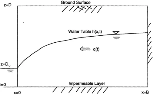
3-2 Schematic representation of an unconfined aquifer . . . . 48
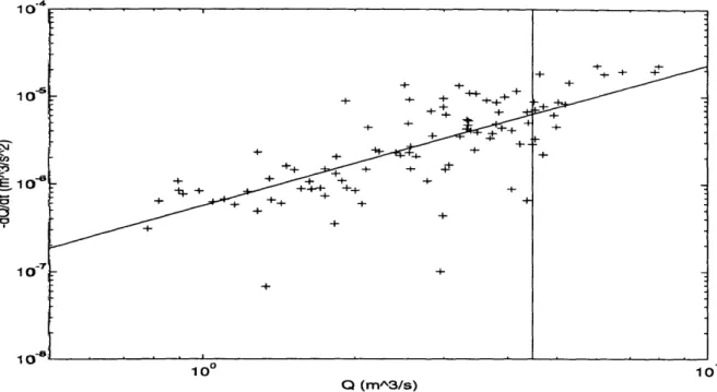
3-3 Recession flow at Souhegan river. Linear regression fitted line and 15% vertical threshold .. .. ... . . ... .... .... 53
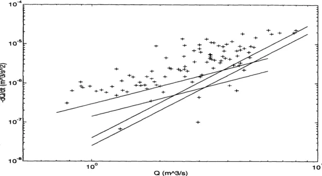
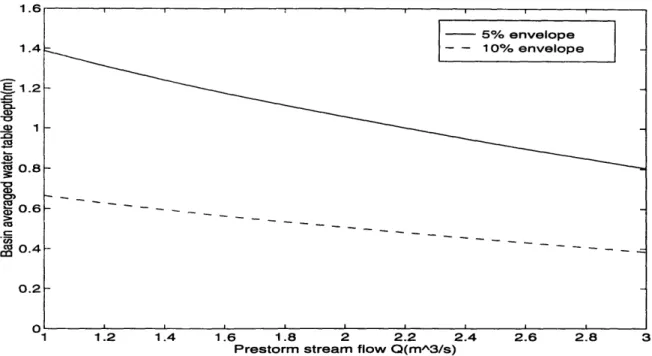
3-4 Recession flow at Souhegan river. The 4 straight lines correspond to 5% and 10% envelopes with slopes 3/2 and 3 respectively . . . . 54
3-5 Sensitivity of water table depth to whether 5% or 10% envelope is used to estim ate a, . . . 55
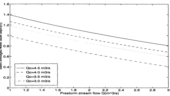
3-6 Sensitivity of water table depth to critical flow rate
Q
. . . ..
563-7 Sensitivity of water table depth to a priori estimated drainable porosity n e . . . . . .. . . 56
4-1 DEM of Rosano ... 63
4-2 Channel network of Rosano . . . . 64
4-3 Soil map of Rosano ... 66
4-4 Rain gauges in Rosano ... 69
4-5 Hydrographs at Rosano for storm of Feb.20-22, 1977 using hourly rain gauge data . . . 71
4-6 Hydrographs at Subbiano for storm of Feb.20-22, 1977 using hourly
rain gauge data ...
...
. 724-7 Hydrographs at Fornacina for storm of Feb.20-22, 1977 using hourly rain gauge data . .... ... .. 72
4-8 Hydrographs at Rosano for storm of Feb.20-22, 1977 using daily rain gauge data ... ... . ... 75
4-9 Hydrographs at Subbiano for storm of Feb.20-22, 1977 using daily rain gauge data ... ... . ... 75
4-10 Hydrographs at Fornacina for storm of Feb.20-22, 1977 using daily rain gauge data ... ... . ... 76
4-11 Hydrographs at Rosano for storm of Jan. 9-10, 1979 . . . . 77
4-12 Hydrographs at Subbiano for storm of Jan. 9-10, 1979 . . . . 78
4-13 Hydrographs at Fornacina for storm of Jan. 9-10, 1979 . . . . 78
4-14 Hydrographs at Subbiano for storm of Nov. 13-14, 1982 . . . . 80
4-15 Hydrographs at Fornacina for storm of Nov. 13-14, 1982 . . . . 80
4-16 Hydrographs at Rosano for storm of Nov. 24-26, 1987 . . . . 82
4-17 Hydrographs at Subbiano for storm of Nov. 24-26, 1987 . . . . 82
4-18 Hydrographs at Fornacina for storm of Nov. 24-26, 1987 . . . . 83
4-19 Hydrographs at Rosano for storm of Oct. 30-31, 1992 using rain gauge data ... ... . . . ... 84
4-20 Hydrographs at Subbiano for storm of Oct. 30-31, 1992 using rain gauge data ... ... . . ... . 85
4-21 Hydrographs at Fornacina for storm of Oct. 30-31, 1992 using rain gauge data... . . ... .... ... ... .. 85
4-22 Rainfall volume at spatial points measured by radar and rain gauges. 87 4-23 Hydrographs at Rosano for storm of Oct. 30-31, 1992 using radar and rain gauge data ... . .... . . ... . 89
4-24 Hydrographs at Subbiano for storm of Oct. 30-31, 1992 using radar and rain gauge data .. ... . 90
4-25 Hydrographs at Fornacina for storm of Oct. 30-31. 1992 using radar
and rain gauge data... ... . ... 90
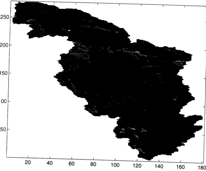
5-1 DEM of Souhegan... . . ... . ... .. 93
•142 Channel network of Souhegan . . . . .. 94
5-3 Soil map of Souhegan ... 96
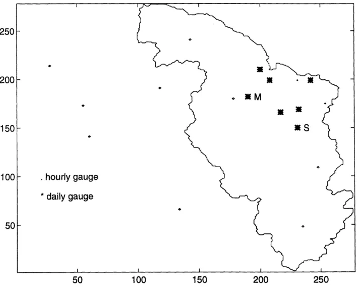
.5-4 Rain gauges within radar coverage ... 99
.5-5 Radar and rain gauge comparison for the storm Sept. 19-20, 1987 . . 102
i-6 Measured and simulated hydrographs for the storm Sept. 19-20, 1987 103 75-7 Radar and rain gauge comparison for the storm June 27, 1987 . . . . 105
5-8 Measured and simulated hydrographs for the storm June 27. 1987 . . 106
!9A Radar and rain gauge comparison for the storm June 22-23. 1987 . . 107
35-10 Measured and simulated hydrographs for the storm June 22-23, 1987 108 t-11 Radar and rain gauge comparison for the storm June 22-23, 1988 . . 109
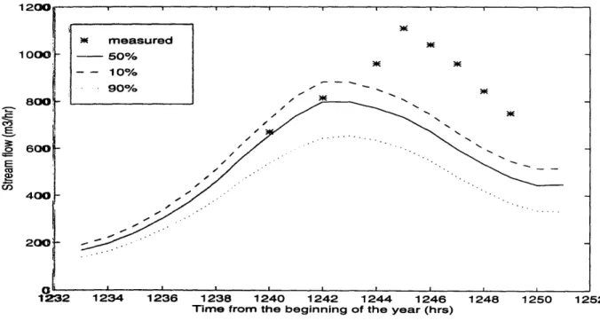
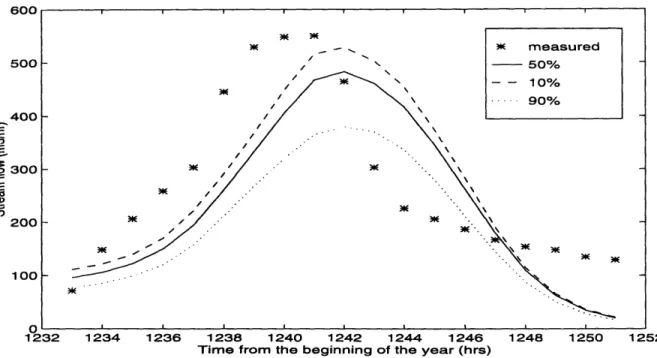
5-12 Measured and simulated hydrographs for the storm June 22-23, 1988 110 •-1 13 Radar and rain gauge comparison for the storm October 21-22, 1988 111 ,.5-14 Measured and simulated hydrographs for the storm October 21-22, 1988112 .- 15 Radar and rain gauge comparison for the storm August 29-30, 1988 . 114 5-16 Measured and simulated hydrographs for the storm August 29-30, 1988 115
List of Tables
3.1 Results with different drainable porosity values ...
3.2 Basin averaged water table depth for the 6 storms ... 4.1 Soil properties in Rosano ...
4.2 Soil properties in Rosano(continued) . . . ...
4.3 Simulations for the storm Feb.20-22, 1977 using hourly rain gauge data 4.4 Simulations for the storm Feb.20-22, 1977 using daily rain gauge data 4.5 Simulations for the storm Jan. 9-10, 1979 . . . .
Simulations for the storm Nov. Simulations for the storm Nov. Simulations for the storm Oct. Simulations for the storm Oct. data . . . .
13-14, 1982 ....
24-26, 1987 . ...
30-31, 1992 using rain gauge data . . 30-31, 1992 using radar and rain gauge
5.1 Soil properties 5.2 Simulation for 5.3 Simulation for 5.4 Simulation for 5.5 Simulation for 5.6 Simulation for 5.7 Simulation for in Souhegan . the storm Sept. the storm June the storm June the storm June
19-20, 1987 .
27, 1987 .. ..
22-23, 1987 . 22-23, 1988 .
the storm October 21-22, 1988 the storm August 29-30, 1988 .
. . . . 97 . . . . . 103 . . . . . 104 . . . . . 106 . . . . . 108 . . . . . 112 . . . . . 113 4.6 4.7 4.8 4.9
Chapter 1
Introduction
A watershed consists of a complex three-dimensional mosaic of soils, vegetation and bedrock, all of which are highly heterogeneous over space. The hydrological processes occurring in a watershed are very complicated. A drop of water may follow an infinite number of pathways between its precipitation on the land surface and its subsequent discharge through stream channels or evapotranspiration (Woolhiser, 1981). However, with the increasing understanding of the hydrological processes and the increasing availability of computer resources, significant advances have been made in developing physically-based, distributed hydrological models during the last two decades.
Unlike the traditional lumped conceptual models which take lumped input pa-rameters and simulate total runoff at the basin outlet, physically-based distributed models simulate the hydrological processes at every point within a basin. In these models, hydrological processes are modeled with the governing principles, either by partial differential equations of mass, momentum and energy conservation, or by em-pirical equations derived from independent experimental researches, such as Darcy's equation for subsurface flow and Penman-Monteith equation for evapotranspiration. Runoff generation mechanisms
The main components into which precipitation may be partitioned are evapotran-spiration. overland flow, unsaturated subsurface flow and saturated subsurface flow. Runoff is influenced by the rainfall intensity and duration, antecedent basin
condi-tions and the basin characteristics, especially the basin topography. In most cases, over a basin scale, the major component of the hydrograph is overland flow.
The generation of overland flow occurs under at least three sets of conditions (Kirkby, 1985). When rain falls faster than it can be infiltrated into the soil, then the excess rainfall will form Hortonian or infiltration-excess overland flow. When the soil is saturated, any further rainfall will generate saturation-excess overland flow. Return overland flow occurs where subsurface flow is forced up to the surface by the soil or slope configuration.
Since the seventies, the concept of variable source area overland flow generation has been gaining more and more attention. This concept implies that during a storm, most rainfall infiltrates into the soil and migrates as subsurface flow downslope to produce saturated areas, mostly near the channel. From these areas overland flow is generated either as saturated overland flow directly from rainfall or as return overland flow. Saturated contributing areas can expand or shrink in response to the changing rainfall intensity. In contrast to the "Hortonian" overland flow concept, the variable source area concept incorporates the entire range of the hillslope processes, rather than only the infiltration process in a vertical soil column.
In urban or other developed watersheds, the Hortonian overland flow may dom-inate the hydrograph, but in forested or wildland watersheds, it is the saturated overland flow and return flow that dominate. Numerous observations have been re-ported to support the variable source area theory. For example, Pilgrim et al. (1978) reported on a field evaluation of surface/subsurface runoff processes under natural and artificial rainfall. They found that the surface flow was mostly a combination of return flow and saturated overland flow, and the Hortonian overland flow was discontinuous downslope and only local in nature.
Development of physically based distributed models
Given the complex three-dimensional nature of the hydrological processes, it is ex-tremely difficult to model them mathematically. Not all of the conceptual under-standing of the way hydrological systems work is expressible in formal mathematical
terms (Beven, 1985). Sometimes hydrological processes are expressed mathematically in the form of non-linear partial differential equations that can not be solved analyti-cally for the cases of practical interest. Numerical solutions must be found, which will involve the discretization of the space-time coordinates. And when the mathematical models are applied to a basin, some simplifications are usually necessary (such as reducing the dimensionality of the processes) to make the problem manageable.
The Institute of Hydrological Distributed Model (IHDM) classifies the watershed into a number of spatial zones of like attributes with respect to vegetation type and microclimate (Calver, 1988). The basic structure of the model calculations is a two dimensional representation of each hillslope section in the vertical slice sense; changes of hillslope width within each section can be incorporated, allowing the effects of converging and diverging hillslope flows to be taken into account. The IHDM assumes that overland flow results from Hortonian runoff and return flows. Channel flow and any overland flow are modeled by the one dimensional Kinematic Wave equation, which is solved using a 4-point implicit finite difference scheme. The unsaturated and saturated flow are modeled together using two-dimensional Richards equation, incorporating Darcy's law and consideration of mass conservation. This equation is solved using a finite element scheme, the Galerkin method of weighted residuals for the two space dimensions and an implicit finite difference method for the time dimension. The interception and evapotranspiration may be derived from modeling or observation, and must be subtracted from rainfall to get net rainfall input.
The Systeme Hydrologique European (SHE) model is one of the most compre-hensive physically-based distributed hydrological models. It simulates the entire land phase of the hydrological cycle (Abbot et al., 1986). In the SHE model, spatial distri-bution of watershed parameters, rainfall input and hydrological response is achieved in the horizontal by an orthogonal grid network and in the vertical by a column of horizontal layers at each grid square. Grid spacing in the horizontal can vary across the network, but must remain the same for a given row or column within the net-work array. Node spacing in the vertical is a function of the vegetation type which characterizes a given grid square and can vary between the root zone and the soil
layer below it. Each primary process of the land phase of the hydrological cycle is modeled as a separate component: interception is modeled by the Rutter accounting procedure; evapotranspiration is modeled by the Penman-Monteith equation: over-land and channel flow are modeled by simplified St. Venant equations; unsaturated zone flow is modeled by the one dimensional Richards equation; saturated zone flow is represented by the two dimensional Boussinesq equation; and snowmelt is obtained using an energy budget method.
The assumptions made in the SHE model are: flow in the unsaturated subsurface zone is essentially vertical and flow in the saturated subsurface zone is essentially hor-izontal. Flows in the soil macropores are secondary details and thus are not explicitly but implicitly modeled. Flow in the confined aquifer is of secondary importance and is not modeled. The one dimensional unsaturated flow columns of variable depths act as a link between the two dimensional overland flow component and the two dimen-sional saturated flow component. These equations are solved numerically for each node in space and at each time step. The time step can be different for different components, but must remain constant in a component.
Most distributed models partition the watershed into small grids like the SHE model. The grid structure typically restrains the flow from one node to one of the eight possible directions and flow paths take on a zigzag shape (Moore and Hutchinson, 1991). Vieux et al. (1988) used a TIN (Triangular Irregular Network) to provide a framework for solving the kinematic forms of the two dimensional overland flow equations using the finite element method. In this application, the quadrilateral and triangular elements were aligned so that the principal slope direction was parallel to one of the sides of the element. This made the flow path representation more realistic. Recognizing the importance of the topography on the basin hydrological responses, the THALES model (Moore and Hutchinson, 1991; Grayson et al., 1992a) assumes that the contour lines are equipotential lines and pairs of orthogonals (streamlines) to the equipotential lines form the "stream tubes". Adjacent contour lines and stream-lines define irregularly shaped elements. Surface runoff enters an element orthogonal to the upslope contour line and exits orthogonal to the downslope contour line, with
the adjacent streamlines being no-flow boundaries. Flow from one element can then be successively routed to downstream elements within the same stream tube.
The model also assumes that the infiltrated water flows downslope in a saturated layer overlaying an impermeable base. and this flow is modeled as one dimensional kinematic flow. If the subsurface flow rate exceeds the capacity of the soil profile to transmit the water, surface saturation occurs and the rain falling on the saturated areas becomes direct runoff. Runoff can also be generated by Hortonian overland flow, which is also modeled as one dimensional kinematic flow. Infiltrated water is assumed to flow vertically through an unsaturated zone to become part of the saturated layer. More recently, Paniconi and Wood (1993) developed a numerical model based on the 3D transient Richards equation describing flow in variably saturated porous media. The equation is solved using the finite element method to simulate the hydro-logical processes at subcatchment and catchment scale. The model can be applied to catchments of arbitrary geometry and topography. The model automatically handles both soil driven and atmosphere driven surface fluxes, and both saturation excess and infiltration excess runoff production.
Runoff generated within a basin varies considerably over space, and this variation occurs at different spatial scales. However, if small area variability is integrated over a large enough area, the effects of the small variations are often attenuated or completely submerged (Grayson et al.. 1992b). The representative Elementary Area (REA), defined as the spatial scale at which the runoff spatial variability disappears, was first proposed by Wood et al (1988). They argue that the internal physical processes within an REA should be studied in detail, and distributed models can use REAs as building blocks to simulate the basin runoff generation. Although there is still an ongoing debate on whether REA really exists, this concept does bring some insight into the issue of spatial variability of runoff generation.
Our understanding and ability to model the hydrological processes is very limited compared to the spatially heterogeneous physical reality. In most of the current distributed models, physical processes are modeled based on the small scale physics of homogeneous systems. In application, we are forced to lump up the small scale
physics to the model element scale (Beven, 1989). The implicit assumption is that the same small scale homogeneous physical equations can be applied at the model element scale with the same parameters. This is a very strong assumption because at a larger scale. some parameters could totally lose their physical meanings. Beven (1989), after examining the fundamental problems with distributed models, concluded that the current generation of physically-based distributed models are. in fact, LUMPED conceptual models. He argued that we need the theory for lumping subgrid processes to spatially heterogeneous grid squares.
In principle physically-based distributed models do not need calibration, because all the parameter values have their physical meaning and are measurable in the field. However, two primary reasons make calibration indispensable for almost all the mod-els before they are applied to a real basin. First, every model has approximations in its representation of the physical processes; second, oftentimes not all the parameter values required by the model are available for a whole basin, some parameter val-ues have to be gval-uessed from experience. Even if they are all available, considerable uncertainty is always associated with these data. Soil properties seem to be most difficult to obtain, not only because that their measurement is financially prohibitive, but also because that they are highly heterogeneous, and the measured values depend strongly on the measurement scale (Beven, 1985).
Physically-based distributed models should be able to predict the internal flow behavior of the basin. However, although there are many models which have reported satisfactory results in representing real basins, most of these "satisfactory results" mean only a good fit of the predicted and observed hydrographs at the basin outlet, or, at most, at only a few other points along the basin channel. But lumped models can altso easily achieve a "good fit" with the observed hydrograph at the basin outlet. Different combinations of parameter values and process presentations could produce similar results at the basin outlet. Thus, it is quite possible to obtain a "good fit" at the basin outlet when representing the wrong physical processes.
WVith all the problems, distributed models still have some advantages over lumped conceptual models. One of the advantages is that we can use a distributed model as a
tool for hypothesis testing (Grayson et al., 1992b), i.e., to assist in the understanding of physical systems by providing a framework within which to analyze data. For instance, the effects of land use change of a basin can be forecasted with a distributed model. Because of the lack of physical significance, lumped models usually need a lot of historically measured data for calibration. Thus in forecasting the hydrological responses of ungauged basins, distributed models will usually perform better than lumped models.
Distributed models represent the future. Spatially distributed topographic and rainfall data (Digital Elevation Maps, or DEM, and radar rainfall data) are becoming more and more available. Remote sensing as a tool has the potential to measure spatially distributed soil parameters (for example, antecedent soil moisture content distribution). Computer resources are expanding every day. Distributed models,
which make the b est use of the distributed topographic, soil and rainfal certainly be the choice of the future, and new ways to solve the existing problems will
be found.
In the following chapters, we demonstrate the applications of a physically based distributed rainfall-runoff model to two river basins of vastly different characteristics. The first river basin, the Arno, is located in Central Italy, we have three streamflow gauges at different parts of the river channel, and rainfall data from raingauges and radar are available. The second river basin, the Souhegan, is located in New England. We use only radar data as rainfall input. It can be shown that with real-time radar data, a physical based distributed model can do a very good job in flood forecasting.
Chapter 2
The Rainfall-Runoff Model
The physically based distributed runoff model used in this work is DBS (Distributed Basin Simulator). It was first proposed by Cabral et al. (1990) and further developed by Garrote (1992). Garrote also wrote all the computer code to make the model actually a flood forecasting system with a very friendly user interface. The system can be run either on-line for real time flood forecasting or off-line for model calibration and basin hydrological behavior studies. This chapter is based on Cabral et al. (1990) and Garrote (1992).
2.1
The One-dimensional Infiltration Model
2.1.1
Assumptions
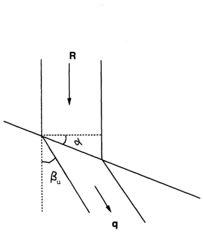
Consider a vertical soil column of horizontal size dX x dY and infinite depth with surface slope angle a (figure 2.1). The reference system is formed by the axes n and p, where n is perpendicular to the terrain surface and positive downward, and p is parallel to the terrain surface and positive downslope. The other axis is Y perpendicular to both n and p.
The flow in the soil is assumed Darcian. The full equations are considered in the saturated area, but the kinematic approximation (Beven, 1984) is adopted in the unsaturated zone, where the contribution of the capillary pressure to the hydraulic
(
Ux
n
q
Figure 2-1: Soil column representation
gradient is neglected (Garrote, 1992). Flow through the macropores in the soil is also neglected. Under the kinematic approximation, the infiltration capacity of the soil column is equal to the saturated hydraulic conductivity at the surface.
Further assumptions include:
(1) The soil is anisotropic with one primary anisotropic direction parallel to the terrain surface p and the other primary anisotropic direction normal to the terrain surface n. The anisotropy ratio is defined as
K,(O8, 0)
ar = Kp(08, 0)
Kn (OS1 0)
where K, (0s, 0) and Kp (9,, 0) are the soil surface saturated hydraulic conductivities
in the n and p directions respectively. ar is assumed to be a constant larger than 1. (2) In the directions p and Y. the soil is homogeneous within the column dX x dY. but in the direction n normal to the soil surface, the soil is heterogeneous with the
d\l
/I
]
soil saturated hydraulic conductivity decreasing exponentially
Kn(0s, n) = Kn(0s, 0)e- fn (2.2a)
Kp(O., n) = Kp(O,, 0)e -fn (2.2b)
where Kn (0s, n) and Kp(9,, n) are the n and p direction soil saturated hydraulic con-ductivities at normal depth n respectively;
f
is a constant expressing the conductivity exponential decay rate.The decrease of saturated hydraulic conductivity with normal depth is a key as-sumption that leads to the formation of perched saturated zone to be described later. Although the decrease may take different functional forms, the exponential form is adopted here. Beven (1982) finds that a number of soil data sets from a variety of basins are well represented by the exponential decay form of saturated hydraulic conductivity.
The Brooks-Corey model (Brooks and Corey, 1964) is used to relate the unsat-urated hydraulic conductivity to the satunsat-urated hydraulic conductivity and moisture content. Using equations (2.2a) and (2.2b), the Brooks-Corey model gives
Kn(9, n) = Kn(Os9, 0)e-n( 0--
)O
(2.3a)Kp(0, n) = Kp(OS, O)e-n( - Or ) (2.3b)
K~(O8,~e 1 0( - Or
where Kn(0, n) and Kp,(9, n) are the n and p direction soil hydraulic conductivities at normal depth n and moisture content 0 respectively; Or is the soil residual moisture content defined as the value below which moisture can not be extracted by capillary forces; 0, is the soil saturated moisture content (porosity); and E is the soil pore size distribution index.
Parameters Or, Os and c are assumed to be constant with depth although hydraulic conductivity is a function of depth. The same approach has been adopted by other authors (e.g., Yeh et al., 1985).
2.1.2
Unsaturated Flow
Using Darcy's equation, the flow vector q can be expressed as (Cabral et al., 1990)
q = -KJnin - KPJPiP (2.4)
where J, and Jp are the n and p direction soil hydraulic gradients respectively, and in and iz are the unit vectors in the n and p directions respectively. Under the kinematic approximations, gravity is the only driving force for moisture flow in the unsaturated zone. Hydraulic gradient is only gravitational,
J = Jnin + Jip = - cos(a)in - sin(a)ip (2.5)
Substituting equation (2.5) into equation (2.4) and from equations (2.1) and (2.3), we have
q = Kn cos(a)in + arKn sin(a)ip (2.6) Because of the soil anisotropy, the unsaturated flow is not in the vertical direction z, but rather it deflects at an angle /., with the vertical direction z(figure 2.1).
It is clear from figure 2.1 that
tan(a + l) = p = a, tan(a) (2.7)
qn
Or we can write
= tan-'(ar tan(a)) - a (2.8)
Angle 0, is constant with depth in the unsaturated zone, and it increases with ar.
Consider rainfall at rate R smaller than the surface normal saturated hydraulic conductivity (figure 2.2), from continuity we can write for steady state unsaturated flow
q= cos() R (2.9)
R
Figure 2-2: Infiltration in the unsaturated soil The steady normal flow is
qn = cos(a + ,03)q = R cos(a) (2.10) Firom equations (2.6) and (2.10) we have
K (O, n) = R (2.11)
Combining equations (2.11) and (2.3a) yields
R
fn
O(R,n) = ()•(O9 - 07) exp( ) + 9r (2.12)
Kn (05 1
0)
f
The above equation shows that under steady state, the moisture content in the unsaturated zone increases exponentially with normal depth in order to maintain the normal hydraulic conductivity equal to the rainfall rate R (Cabral et al., 1990). At
a critical depth N*, the soil becomes saturated and a perched saturated zone starts to develop. This depth N* also corresponds to where the saturated normal hydraulic conductivity equals to the rainfall rate.
Kn(Os, N*) = R (2.13)
Substituting into equation (2.2a), and solving for N* yields
1
K.
(OS,
0)
N*(R) = ln(Kn ) (2.14)
f R
the above equation applies only for the case R < Kn(O0, 0). For R > K,(O0. 0), the saturation is at the surface, no unsaturated zone exists above the wetting front.
Substituting equation (2.11) into equation (2.6) yields
q = Rcos(a)in + a, R sin(a)ip (2.15)
Vertical and horizontal components of the flow in the unsaturated zone are, respec-tively (Cabral et al., 1990),
qz qn cos(a) + qp sin(a) = R[cos2() + ar sin2(a)] (2.16)
and
qx= -qn sin(a)+ qpcos(a) = Rcos(a) sin(a)(ar - 1) (2.17) Both vertical and horizontal components of the flow are constant with depth in the unsaturated zone. For anisotropy ratio greater than one, horizontal flow goes in the downslope direction (Cabral et al., 1990).
2.1.3
Saturated Flow
For a given rainfall rate, as the wetting front penetrates beyond the critical depth N*. the infiltration capacity (the saturated normal conductivity at that depth) of the soil
becomes less than the recharge rate from above, and moisture starts to accumulate above the wetting front. A zone of perched saturation develops and grows both downward and upward. The top of the perched saturation zone is defined as the top front. It is assumed that both the wetting front and the top front proceed perpendicular to the soil surface.
Within the zone of saturation, the soil moisture content is constant. Since we also assumed that all derivatives in the p direction are zero, the continuity equation becomes (Cabral et al., 1990)
Oqn -q= 0
(2.18) On
Equation (2.18) means that the qn is constant in the n direction within the sat-urated zone. Since the gravitational gradient is constant and hydraulic conductivity decreases with depth. constant normal flow implies a positive pressure buildup within the saturated zone to compensate for the different hydraulic conductivities of different soil layers.
J = Jnin + Jip = (-cos(a) + n )in - sin(a)ip (2.19)
where T is a positive pore pressure varying only with normal depth. The flow equation in the saturated zone is
q = qnin+qpip = -Kn(Os, n)Jnin-KP(O,, n)JpiP = -Kn(O7, 0)e-fn Jnin-Kp(Os, 0)e-fn Jip
(2.20) The normal component of the saturated flow can be written as
qn(n) = (cos(a) - O'n )Kn(9, O)e-fn (2.21)
Substituting equation (2.21) into equation (2.18) yields
-[(cos(a)
-)Kn(9
8
, 0)e-fn]
= 0
On On
or
On2 cos(a) 0 (2.22)
This equation governs the pressure distribution within the saturated zone.
Pressure at both top and wetting fronts can be assumed atmospheric given that they are in contact with the unsaturated zones. Integration of equation (2.22) with this boundary conditions xI(Nf) = xF(Nt) = 0 leads to
1 - en
(N
1 efn - ef t(n) = cos(a) (n + eN - ef (Nt + - efNf - efNt (Nf + )] (2.23)
where Nf and Nt are the normal wetting and top front depths respectively. Substituting equation (2.23) into equation (2.19) yields
J = -[f(N Nt) e/n ] cos(a)in - sin(a)ip (2.24)
ef N. -- ef Nt
And substituting equation (2.23) into equation (2.21) yields
f (Nf - N)
qn
= Kn(0.,0) e
-
e) cos(a)
(2.25)
eNf - ef Nt
We can define an "equivalent hydraulic conductivity" for the saturated zone, Keq, as the normal hydraulic conductivity of a homogeneous soil column with the same normal flow qn given by equation (2.25) (Garrote, 1992),
)f(Nf- Ne)
Keq(Nf Nt) = K(Os, 0) e- f(Nf -fNf_ N~fNtNt) (2.26)
This Keq also corresponds to the harmonic mean of the soil normal hydraulic conduc-tivities over the saturated depth
fN ' dn
Keq(Nf , Nt) N= dn
Nt Kn (0,,n)
We may also define "equivalent depth", Neq, the normal depth where the normal saturated hydraulic conductivity equals to Keq(Nf , Nt). From equations (2.2a) and
(2.26),
Neq(Nf, Nt) n_ f f(Nf -f Nt)] (2.27)
X~~q(X:,
Xe) = 7 •Nf
-
efNtn
Figure 2-3: Pore pressure profile in the perched saturated zone
Neq is also the depth at which the pore pressure is maximum (equation (2.23)) (fig-ure 2.3). For Nt < n < Neq, the saturated hydraulic conductivity is greater than
Keq, and the pressure gradient is positive downward to compensate for the exces-sive hydraulic conductivity and maintain constant normal flow. For Neq < n < Nf,
the saturated hydraulic conductivity is smaller than Keq, and constant normal flow implies a negative pressure gradient downward.
The parallel component of the flow is
qp = Kp(Os,. 0)e- f n sin(a) (2.28)
Between the wetting and the top fronts, normal flow is affected by the pressure gradient in the normal direction while parallel flow is not. And also due to the soil anisotropy, the saturated flow is deflected laterally. The angle of flow with the vertical
I\
direction : is designated 3s, which is a function of normal depth:
efNf ef N
tan(a + /3s(n)) = qp = a, tan(a) e e _f (2.29)
qn f (Nf - Nt)
Solving for 3,(n) gives
efNf - efNt
0,(n) = tan-'[a, tan(a)f(N - N)f e -IN ] - a (2.30)
f (Nf - Nt)
The vertical and horizontal components of the flow in the zone of saturation are, respectively.
qz (n) = qn cos(a)+qp sin(a) = [Kn(0s. 0)f(Ne - Ne) cos(a)] cos(a)+[K,(0s, 0)e- f sin(a)] sin(a)
ef N1 - ef't
or
orf (Nf - Nt) 2
qz(z) = Kn(Os, 0)[ar e -fzcs(a) sin2 (a) + ef Nj - ef Nt COS2(a)] (2.31a)
and
q, (n) = -qn sin(a)+qp cos(a) = -[K,(0,, 0) f(NI efN - Nt) cos(a)] sin(a)+[Kp(0, 0)e- fn sin(a)] cos(a
1 - efNt
or
qx (z)
=
Kn (Os,
0) sin(a) cos(a) [are-fz cos(a)
f(Nyf-
(2.31b)
ef Nf - efNt
Because of the flow deflection in the saturated zone, the vertical infiltration is not constant with depth. It is the sum of a constant term and a term which decays exponentially with depth. The resulting horizontal flow may be negative (upslope) as well as positive (downslope), depending on the relative values of ar,
f,
z, ac, Nf andn.
Nr
n
Figure 2-4: Integration domain Q for the continuity equation
2.1.4
Wetting and Top Front Evolution
Wetting front before perched saturation
Under steady infiltration, the soil moisture profile in the unsaturated zone is given by equation (2.12). Prior to a storm the initial moisture profile is assumed to be given also by equation (2.12) with R equal to a very small initial recharge rate Ri. Consider a constant rainfall rate R, R > R, over a given interval, a sharp discontinuity in the moisture content separates the area affected by the propagation of the infiltration wave and the undisturbed area below the front.
Assume: (1) equation (2.15) is valid for the area just above and below the wetting front; (2) the wetting front is parallel to the surface and advances perpendicular to
The continuity equation can be written as
00 08q &qp 0- + 0qn + Op - 0
(2.32) at an OP
Integration of equation (2.32) in the domain Q (enclosed by p = pl, p = p2, n = n1 and n := n2) (figure 2.4) gives
( O
+ + )d
()dQ
+ (
+
q)d
= 0
(2.33)
Interchanging the integral and the derivative in the first term and applying Green's theorem to the second term gives
d ( OdQ) + (q.iZN)d(sQ) = 0 (2.34)
where i: is the unit vector normal to the boundary of Q, sQ. The time rate of change in moisture content within Q is balanced by the flux ( across its boundary sQ.
Above and below the wetting front, the soil moisture profiles are given by equation (2.12) with infiltration rate equal to R and Ri respectively. Thus
SOda•
j2 jf20(n)ddp
=
(P2 - p)
[ 0(o)dn
+
J
(n)
dn]
- (P2 P1)[(Kn(s,0) ) (Os - Or)()(e{Nf i- e') + Or,(Nf
- )+
Ri
( (,) ) s - Or)S( ) (e n2 - E N ) r(72 _ fS)] (2.35)
and d fff
R 1-( ~ r
d-( Oda) -- (P2-pl)[Kn(Rs, O)) (Os -- Or)eNf I+ Or]
K(0, 0) ) (s - Or)e +Or} dNt
The second term of equation (2.34) can be expanded as
n
f2 - 2 nf2
(jiiN)d(sQ) l- p=,dn - qn ln=nldP + qpP=P2dn + qn n=2dp
SO pp 1 n pl
Since the flow parallel to the hillslope is constant with depth
qP=P =qP P=P2Vn
we have
f
P2 P2.i)d(s) = - qn n=ndp+ qnln=n2dp (2.37)
•'l 1 91
For n < Nf, qn is given by equation (2.10), and for n > Nf, qn is also given by equation (2.10) with R = Ri. It then follows that
j( .iN)d(sQ)
= -Rcos(a)(p 2 - pl)+
Ri cos(a)(p2 - P1) (2.38)Substituting equations (2.36) and (2.38) into equation (2.34) and after manipulations yields
dNf (R - Ri) cos(a) N*
dt O(R, •) - 0(R N1)' N < N*(R) (2.39)
dt
0(R, Nf) - 0(Rj, Nyf)'
Equation (2.39) governs the advancement of the wetting front before perched saturation develops, that is, before Nf reaches the critical depth N*(R). Since when
NV < N*(R), the top front is the same as the wetting front, equation (2.39) is also
valid for the top front evolution.
It can be seen that the wetting front advancement velocity depends on the differ-ence between the rainfall rate and the initial recharge rate and the differdiffer-ence between the moisture distributions corresponding to R and Ri at the wetting front.
Wetting and top fronts in perched saturation
After the wetting front reaches the critical depth N*(R), the evolution of N1 can
be similarly obtained through integration of the continuity equation. The domain of integration is now defined by Nt < ni1 < N1 < n2. Normal flow is given by equation
(2.25) at n = ni (saturated zone) and by equation (2.10) at n = n2 (initial recharge
zone). The result is
dN K, (01, 0) fe(' - R,
dNf
_ TN- -,fNdt= - O( NV) cos(a), Nf > N*(R) (2.40)
dt 0, - 0( Ri, .f )
Derivation of the evolution of the top front is similar to that of the wetting front. The domain of integration is now defined by ni < Nt < n2 < Nf. Normal flow is
given by equation (2.10) at n = n, and by equation (2.25) at n = n2. The result is
dNt d. Kn (Os, 0) f -'N - R
- R-e N cos(a), Nt > 0 (2.41) dt 0s - O(R, Nt)
Since Rcos(a) > q, = K(Os, 0) eX__f f(N-Nt) f• Nt cos(a), the time derivative of Nt is
negative. N, normally decreases until it reaches the terrain surface. Eventually whenNt reaches the surface, we have
dNt= 0, Nt
= 0 (2.42)
dt
2.2
Basin Scale Model
The one-dimensional infiltration model is formulated for a constant rainfall intensity in a uniform slope of infinite length. Water moves in the plane defined by the vertical direction and the direction of maximum slope (p direction). Lateral inflow is balanced by lateral outflow for each vertical section. When this one-dimensional model is applied to a basin scale, many difficulties arise. First, water does not move just in a plane, but rather, the flow is truly 3-dimensional. Second, Even if the flow is confined in a plane, water will accumulate or deplete at certain points because of different slopes and different soil properties, and this accumulation and/or depletion will affect the wetting and top front evolutions. Third, rainfall rarely, if ever, occurs with constant intensity in time or space. To deal with these difficulties, further assumptions and modifications have to be made.
2.2.1
Equivalent rainfall rate
The basin is horizontally discretized into small square elements called pixels. Each pixel is treated as a soil column within which the one-dimensional model is applicable. The temporal variation of the rainfall intensity in one pixel can be treated by assuming that water gets redistributed in the normal direction so quickly that only a single moisture wave propagates downwards despite the variability of the rainfall intensity during a storm. This assumption, although strong, is supported to some extent by the way the unsaturated infiltration mechanism redistributes moisture (Garrote, 1992). With a variable rainfall intensity, if moisture content at some depth is higher, the hydraulic conductivity will be higher, and moisture will tend to migrate from that point. Conversely, if moisture content is lower at some depth, moisture will tend to accumulate.
For each computation step and for each pixel, a moisture balance is performed to derive the moisture content (see next section). We define an equivalent uniform rainfall rate Re as that which would lead to the same moisture content in the unsat-urated part of the soil column. The soil moisture profile is given by equation (2.12). Integrating equation (2.12) above the top front and equating it to the unsaturated moisture content MA, we get
fo
o K(O,0)
Re )Re 0 (8( - Or)er: +Or,]dn = M,and solving for Re yields
M - Ort
(2.43)
Re
= Kn(Os, 0Y [
f"
2.3
(Os - Or)-(e- - 1)
where MI is the total storm moisture content inside the soil column above the top front.
Equation (2.43) is valid only when there is an unsaturated part in the pixel. When the top front is at the surface (Nt = 0), the equivalent rainfall rate is the actual rainfall rate at that time step.
2.2.2
Moisture Balance
The lateral moisture fluxes between neighboring pixels pose another difficulty. The
lateral moisture flux, the vertical flux, the moisture content and the hydraulic po-tential of the soil within a pixel are functions of one another. The three-dimensional equation of moisture flow is needed to fully account for the moisture exchange be-tween pixels. However, to reduce the computation burden to the extent bearable for real-time flood forecasting, simplifications must be introduced.
The simplifications adopted are based on the idea of decoupling the vertical and horizontal moisture flow equations. Two mechanisms of lateral moisture transfer are considered. First, when the one-dimensional model is applied to a bounded domain,
the horizontal component of flow produces a net moisture flow at the downslope
boundaries, which is transmitted to the contiguous element. Additionally, the ap-plication of the one-dimensional model independently to each element gives different pressure and moisture distribution to every element, which, in turn, leads to horizon-tal hydraulic gradients that drive lateral flow between elements (Garrote, 1992).
Lateral flow in homogeneous terrain
In the one-dimensional kinematic model of infiltration, local slope, anisotropy and
vertical heterogeneity produce a diversion of the infiltration from the vertical direc-tion. Thus lateral moisture movement exists. For an infinite homogeneous slope, the moisture flow is not affected by the boundary conditions. However, for a finite domain, the boundary conditions will in general have great influence on the flow. The influence is treated rather simply here.
The one-dimensional infiltration equations are assumed to be valid at the subgrid scale. The horizontal component of the flow can be integrated vertically from the surface to the wetting front to obtain the net flow across the boundary (Garrote,
1990).
Qh = W Jo q, (z)dz
cross-section. This equation can be evaluated as
Qh = W[f - q(z)dz + COS() qx(z)dz] (2.44)
cos(a )
Substituting equations (2.17) and (2.31) into equation (2.44) yields
Qh = W sin(a) ){[NtR(a, -1)]+ [K, (Os, O)a (e-fNt - e-f I)]- [K (Os, 0)fNf - Nt)2
(2.45)
For a rainfall rate lower than the initial infiltration capacity (R < Kn(OS, 0)), lateral discharge is given only by the first term of equation (2.45) while Nt = NJ <
N*(R). After perched saturation has developed (Nt < Nf), lateral discharge is given by all the three terms of equation (2.45). And eventually when saturation reaches the surface (Nt = 0), the lateral discharge is given only by the second and the third term of equation (2.45).
The lateral flow across the cross-section is evaluated for every element in the basin. Subsurface inflow into a given element is given by the sum of the outflow from all its upstream elements draining directly into it. The computations are carried out recursively according to the relation "drains to" (Garrote, 1992). This means that the outflow from all the upstream elements should be computed before computing the outflow from a given element.
The simplifications made are: (1) Boundary effects are neglected. The one-dimensional model is applied to the central point of every element, and each element is considered effectively an infinite extension of soil. (2) The influence of lateral mois-ture flow on the momentum equations is neglected, although the mass conservation is taken into account. The equations governing the evolution of wetting and top fronts are affected only indirectly by the lateral moisture balance (through the equivalent rainfall rate). (3) The flow entering every element is assumed parallel to its line of maximum slope, irrespective of the orientation of the slopes of the upstream elements.
Lateral flow due to spatial variability
The horizontal hydraulic gradients between elements are usually very small because the horizontal distances between elements are typically very large. Therefore, the lateral flow due to spatial variability of pressure is small compared to the lateral flow due to topography and anisotropy (Garrote, 1992).
Again, the one-dimensional model is applied to the central point of every element independently. The pressure distribution along the normal direction is estimated for every element. The lateral hydraulic gradient between two contiguous elements is
given by
J (z) = •A9(z)
OX
AX
T2(z) - TI(z) (2.46)X2 - X1
where * is the pore pressure, z is the vertical depth, and x is the horizontal distance. The assumptions made are: (1) The effects of different depths of the perched saturation at contiguous elements are neglected. (2) The effects of different slopes at contiguous elements are neglected. Thus the normal directions to the terrain surface at two contiguous elements are assumed parallel to each other, and Ax is independent of z. Hence the vertical depth z can be substituted by ', where a is the average slope angle of the two elements.
Using Darcy's equation, we get the lateral flow
qx(z) = -Km(z)Jx(z) (2.47)
Because of the spatial heterogeneity, two contiguous elements may have different soil hydraulic conductivities inside a basin. The equivalent hydraulic conductivity in the horizontal direction, Km(z), for the inter-element distance Ax is approximated by the equivalent hydraulic conductivity in the parallel direction, which, in turn, corresponds to two elements of length Ax/2 connected in series
1
1
1 1-+
(2.48)
Km(z) 2KP (O0, z) 2K2 (O0, z) (2.48) The total lateral flow resulting from the spatial variability of pressure can be
obtained by integrating equation (2.47) along the saturated depth Q = - Js,, Km(z) Jx (Z)dz (2.49) nf where
NI
N ,
Zinf = mi( f)
cos(ce) cos(a)
and zsp = min( Nt Nt2 Scos(a)' cos(a)
Substituting equation (2.46) into equation (2.49) yields,
QX
=
sKm'(z)
-()
dz
zrnf SN f 'N fl XF (Z()" = cos( K z ) dz coscm Km (z) z 2dz (2.50) JNt. _X_(250)
cos(a) cos(a)The lateral flow of moisture due to the spatial variability of pressure can be com-puted as the difference between the flows that would result considering pressure dis-tribution in both pixels independently. Substituting equations (2.23) and (2.48) into the first term of equation (2.50) and considering a cross-section of width W yields the moisture outflow from element 1
W NtefNf - NfefNt 1 Nf + Nt
Qpout = Kp(Os 0) (N - Nt )[ + (2.51)efN
X2 - XI f
4
All the variables in the above equation refer to element 1 only. The second term of equation (2.50) which represents the moisture inflow into element 1 can be derived similarly.
The total moisture outflow from a given element is the sum of equations (2.45) and (2.51), and the total moisture inflow to a given element is the sum of the moisture outflow from all the upstream elements that drain directly to it.
2.2.3
Runoff Generation
Two modes of runoff generation are represented in DBS: infiltration excess runoff and return flow (Garrote, 1992). The infiltration excess runoff is a direct consequence of pixel states, and return flow is the result of the global moisture balance in the soil column.
Pixel states
Depending on the positions of the top and wetting fronts, a soil element can be in any of the four different moisture states, which have different runoff generation potentials (figure 2.5)
Unsaturated state: The wetting front is at some depth above the water table, and perched saturation has not developed yet, the wetting and top fronts are the same. The soil column generate infiltration excess runoff only.
Perched saturated state: The wetting front has penetrated beyond the critical depth N*, and the top front is separated from the wetting front but has not reached the surface. The soil column can generate infiltration excess runoff.
Surface saturated state: The wetting front has not reached the water table, but the top front has reached the soil surface. The soil column generates infiltration excess runoff. It may also generate return flow if infiltration plus subsurface inflow exceed subsurface outflow plus the storage increment due to the progression of the wetting front.
Fully saturated state: The wetting front has reached the water table and the top front has reached the soil surface. Both infiltration excess runoff and return flow are generated.
Infiltration excess runoff
The infiltration capacity of a soil column is a function of the wetting and top front positions. When the rainfall intensity is higher than the infiltration capacity, infil-tration excess runoff is generated. For unsaturated (Nf = Nt) and perched saturated
Perched saturated
Osat esat
Surface saturated Fully saturated
sat
Figure 2-5: Different pixel states
Unsaturated
V
v
(0 < Nt < Nf) elements, the infiltration capacity is only controlled by the surface saturated hydraulic conductivity,
Imax = K (0s, 0) cos(a) (2.52) where Imax is the infiltration capacity of the soil column.
For surface saturated elements (Nt = 0, Nf < Nt), the infiltration capacity is the harmonic mean of the saturated normal hydraulic conductivities of the saturated depth. From equation (2.26) we have
fNf
Imax = K(0s, 0) fN - 1 cos(a) (2.53)
Imax is controlled by the whole perched saturated zone from the surface down to the
wetting front, rather than just by the surface layer.
For fully saturated elements (Nt = 0, Nf = Wt), only the inter-storm recharge rate R, can be maintained, no storm rainfall can infiltrate to the soil column.
Imax =0 (2.54)
The actual infiltration I is given by
I = R,R < Imax
I = Imax,
R
> Imax (2.55)And the infiltration excess runoff rate Rinf is given by
Return flow
The moisture balance equation for one element during one time step can be written as
dMt - dNf•O(Ri, Vf) + I + Qlin -Qlout
(2.57)
dt dt A
where Mt is the total moisture content above the wetting front, Qtin is the lateral moisture inflow, Qlot is the lateral moisture outflow, and A is the horizontal area of one element. The change of Mt in an element is the result of infiltration, lateral moisture exchange, and the incorporation of the initial moisture due to the vertical displacement of the wetting front. 0(R/, Nf) can be evaluated with equation (2.12).
It is assumed that all the moisture inflow accumulates above the wetting front. Therefore, M't has an upper limit set by Nf 0, corresponding to surface saturation
(Garrote, 1992). Whenever the sum of the previous moisture content plus the net moisture inflow exceeds this limit, return flow is generated, and the return flow rate
during tj - to is
ftl dNf Qua - Q1out
Rr = {Nf(t)Os - Mt(to) - [- 0(R 1, N) I+ I -AQo ]dt}/(tl - to) (2.58)
The total runoff generation rate Rf by one element is
Rf = Rinf + R, (2.59)
2.2.4
Surface flow routing
The runoff generated by each grid inside the basin has to be routed to the basin outlet to get the actual hydrograph of a storm event. The path that the runoff generated at every grid point follows can be derived from the DEM according to the rule that water drains to the lowest of its 8 neighboring grids. For a hillslope pixel, the path consists of two parts: the hillslope part and the channel part; and for a channel pixel, the runoff only follows a channel path.