Design of an Automated Purification System for Biologically-Active
Macromolecules
by
Eric Hoarau
B.S., Mechanical Engineering
University of California at Berkeley, 1999
Submitted to the Department of Mechanical Engineering
in partial fulfillment of the requirements for the degree of
Master of Science in Mechanical Engineering
at the
MASSACHUSETTS INSTITUTE OF TECHNOLOGY
June 2001
© Massachusetts Institute of Technology 2001
All rights reserved
ENO
MASSACHUSETTS INSTITUTE OF TECHNOLOGYJAN 2 3 2002
LIBRARIESSignature of A uthor ...
...
Department of Mechanical Engineering
May 11, 2001
C ertified by ...
...
...
...
Kamal Youcef-Toumi
Professor of Mechanical Engineering
Thesis Supervisor
Accepted by ...
Ain A. Sonin
Design of an Automated Purification System for Biologically-Active
Macromolecules
by
Eric Hoarau
Submitted to the Department of Mechanical Engineering on May 11, 2001, in partial fulfillment of the
requirements for the degree of
Master of Science in Mechanical Engineering
Abstract
All biologically active macromolecules (BAMs) including pharmaceutical drugs need
purification as part of their production process to ascribe therapeutic properties. Therefore, the purification of BAMs has proven to be one of the fundamental challenges in drug production and discovery. There are different types of techniques presently being used to purify BAMs: manual, mechanical, or a combination of the two. Although purification techniques have improved dramatically in the last few years, the labor hours, chemicals used, delays and imprecision are still limiting factors.
This thesis first presents a stain-free ultraviolet absorption detection method that can be used to detect a variety of biologically active macromolecules in an electrophoresis gel. Next, it describes the design of a system that will automate the recovery and storage of samples from an electrophoresis gel.
The following components, which were designed and built for this system, are described in this thesis. An ultraviolet light source outputs a wide, collimated monochromatic beam of light to detect specific molecules within the gel. A mechanical cutting device excises bands of various shapes and sizes from an electrophoresis gel. A transportation system was developed to rapidly move the cutting device between the different stations. A cleaning station was implemented to clean and store the cutting tips that are used to excise the gel. Finally, a temperature-controlled storage station was developed to store the excised samples until needed for further analysis.
Thesis Supervisor: Kamal Youcef-Toumi Title: Professor of Mechanical Engineering
Acknowledgments
Thank you Professor Kamal Youcef-Toumi for supervising this thesis and for your support and guidance during my time at MIT. I would like to extend my gratitude to Alpine Pharmaceuticals, Inc. for funding this research. In particular, I would like to thank Dr. Manzoor Shah for his assistance in completing this work.
I would like to thank Belal, Bernardo, Byron, Namik, and Osamah for their help on this
project. I also thank my colleagues in the Mechatronics Research Laboratory and the Intelligent Machine Laboratory who have made my time there enjoyable. Thanks to Leslie and Carolyn for their help with cumbersome MIT paperwork. I would also like to thank Arin, May-Li, and Mike for proofreading this thesis.
Contents
Chapter 1
Introduction...13
1.1 Background Inform ation... 13
1.2 Gel Electrophoresis Principle ... 14
1.3 Purpose of the Research... 16
1.4 Functional Requirem ents and Scope of Research... 16
1.4.1 Functional Requirem ents... 16
1.4.2 Scope of Research ... 17
Chapter 2 D ifferent V isualization Techniques... 18
2.1 Overview ... 18
2.2 Laser Induced Fluorescence (LIF) ... 20
2.3 UV Absorption...22
2.4 Com parison ... 24
2.5 Proposed Technique... 25
Chapter 3 Presentation of the M ain C om ponents... 26
3.1 Overall Overview ... 26
3.2 Detection System ... 27
3.3 Precision X Y stage...28
3.4 Variable Light Source ... 29
3.4.1 Specifications ... 29
3.4.2 Existing D esigns... 3 1 3.4.3 Lam p Choice ... 33
3.4.4 Different Approaches to Filtering ... 38
3.4.6 Optical Com ponents... 45
3.4.7 Final D esign and Lam p Characteristics ... 55
3.4.8 Recom m endations and Future W ork... 61
3.5 Cutting Tool...65
3.5.1 Specifications ... 65
3.5.2 Existing D esigns... 65
3.5.3 Possible D esigns... 66
3.5.4 D esign of the Cutting device... 68
3.5.5 Results and Recom m endations... 71
3.6 D esign of the Cutter Transportation System ... 74
3.6.1 Requirem ents...74
3.6.2 Possible D esigns... 74
3.6.3 D esign of the Transportation System ... 75
3.6.4 Results and Recom m endations... 77
3.7 Cutting Tips Changing Station... 78
3.7.1 Requirem ents...78
3.7.2 D esign of the Tool Changing Station... 78
3.7.3 Results and Recom m endations... 80
3.8 Cutting Tip Cleaning Station ... 82
3.8.1 Requirem ents...82
3.8.2 Possible Cleaning M ethods ... 82
3.8.3 D esign of the Cleaning Station... 84
3.8.4 Results and Recom m endations... 85
3.9 Tem perature Controlled Sam ple Storage Station ... 90
3.9.1 Requirem ents...90
3.9.2 Design of the Temperature Controlled Storage Station ... 90
3.9.3 Results and Recom m endations... 92
Chapter 4 C onclusion ... 97
A ppendix A ...
101
A l M achine Pictures ... 102
A2 Parts List ... 104
A3 Vendors Inform ation... 108
A4 Circuit Schem atic of Selected Components ... 110
A ppendix B ... 112
B CCD Cam era Specifications... 113
B2 XY Stage Specifications... 116
Appendix C The Light Source ... 118
Cl Assembly Drawings ... 118
C2 Parts Drawings... 123
C3 Purchased Parts... 147
Appendix D The Excision D evice...151
Dl Assembly Drawings...151
D2 Parts Drawings...153
D3 Purchased Parts... .... 160
D4 The protean 2-D Spot Cutter by Bio-Rad... 161
Appendix E The Excision D evice Transportation System ... 162
El Derivations for the transportation system ... 163
E1.1 System Torque Calculation... 163
E1.2 Calculation of System Resolution and Speed ... 165
E1.3 Calculation of Rack and Pinion Specifications... 165
Appendix F
The Cutting Tip Changing Station...172
F l P art D raw ings... 172
Appendix G The Temperature Controlled Storage Station...179
GI Derivations for the Temperature Controlled Station ... 180
G1.1 Heat Load Calculations ... 180
G1.2 Calculation of Additional Parameters ... 181
G1.3 System Parameters ... 182
G2 Thermoelectric Cooler Data Sheet... 183
G3 Assembly of the Thermoelectric Cooler Storage Station ... 184
Appendix H The System Software Interface...186
List of Figures
Figure 1.1: Schematic of the electric field between two parallel plates ... 14
Figure 1.2: M acromolecules mobility in matrix gel versus size... 15
Figure 1.3: Example of separation of molecules using electrophoresis... 15
Figure 2.1: Typical LIF detection system [3]... 20
Figure 2.2: Instrumental set-up of a capillary electrophoresis system. [2]... 21
Figure 2.3: Absorption of light by a sample. [4] ... 22
Figure 2.4: CCD based DNA detection in systems for electrophoresis gels. [9]... 24
Figure 2.5: Quantum Efficiency of several CCD Arrays... 25
Figure 3.1: Drawing of the purification system... 26
Figure 3.2: Detection system by: a) taking a picture, b) scanning the gel... 27
Figure 3.3: 402 LN series XY table from Daedal. [4]... 28
Figure 3.4: Double stranded DNA absorbance spectrum. ... 29
Figure 3.5: Absorbance and light source spectra... 30
Figure 3.6: Spectroscopic light system... 31
Figure 3.7: 254nm Ultralum transiluminator... 32
Figure 3.8: Proposed light source... 32
Figure 3.9: Comparison of lamp output stability... 33
Figure 3.10: Spectrum of the L2D2 deuterium lamp using the CCD detector. ... 34
Figure 3.11: Deuterium lamp test: a) apparatus, b) and c) test results... 35
Figure 3.12: Lamp intensity at 254nm versus the angle... 36
Figure 3.13: Lamp intensity versus the angle for each bulb... 37
Figure 3.14: Filter wheel approach... 38
Figure 3.15: Variation of wavelength with incidence angle... 39
Figure 3.16: Diffraction grating approach ... 39
Figure 3.17: Diffraction grating [11]... 40
Figure 3.18: Grating driving mechanism. [11]... 41
Figure 3.19: Overlapping of spectral orders [11] ... 41
Figure 3.20: Plane grating mounts. [11]... 42 Figure 3.21: Concave grating mount [11]...
Figure 3.22: Optics set-up to focus and collimate the light ... 45
Figure 3.23: Light source set-up using a reflector... 46
Figure 3.24: Light source set-up with direct grating's illumination... 47
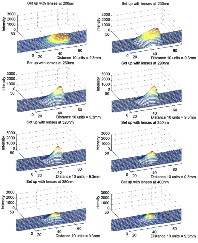
Figure 3.25: Light source illumination at different wavelengths for set-up with lenses. ... 49
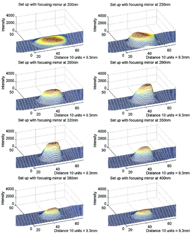
Figure 3.26: Light source illumination at different wavelengths for set-up with reflector... 50
Figure 3.27: Light source illumination at different wavelengths for set-up with direct illumination... 51
Figure 3.28: Light source spectrum analysis for three different focusing set-ups... 52
Figure 3.29: Proposed light source ... 55
Figure 3.30: Set-up to measure unwanted reflected light. ... 58
Figure 3.31: Influence of bare aluminum walls on the output signal. ... 58
Figure 3.32: Output power of the variable light source... 59
Figure 3.33: Illumination profile of light source at 260nm. ... 60
Figure 3.34: Peak location throughout the beam ... 60
Figure 3.35: Possible Gaussian addition to explain the spectrum shape ... 61
Figure 3.36: Deuterium lamp light path ... 61
Figure 3.37: Direct illumination with a baffle to restrict the light reaching the grating... 62
Figure 3 38: Results from testing the influence of the baffles on the direct illumination set-up... 63
Figure 3.39: Projecting type deuterium lamp. ... 64
Figure 3.40: Potential design of the cutting device using a:... 67
Figure 3.41: The cutting device... 69
Figure 3.42: T he cutting tip ... 71
Figure 3.43: Cutting tips cross section ... 72
Figure 3.44: Band expulsion test result ... 72
Figure 3.45: Possible modifications of the cutting tip expulsion system ... 73
Figure 3.46: Transportation systems: a) pulley-belt, b) lead screw, c) rack-pinion ... 74
Figure 3.47: The cutter transportation system... 75
Figure 3.48: The cutting tip storage station... 79
Figure 3.49: Tool changing station solenoid input voltage versus time ... 81
Figure 3.50: Other designs to increase number of stored cutting tips ... 81
Figure 3.51: Different cutting tip cleaning methods... 83
Figure 3.52: The UC-1 ultrasonic cleaner ... 85
Figure 3.53: Ultrasonic cleaner assembly using one beaker for cleaning and one for rinsing ... 89
Figure 3.54: Schematic of a thermoelectric cooler ... 90
Figure 3.56: Temperature on the thermoelectric cold side during power-up and power-down... 92
Figure 3.57: Temperature at a height of 10-mm with different heat transfer materials... 93
Figure 3.58: Cooling test, temperature at a height of 10-mm with an aluminum block... 95
Figure 3.59: Heating test, temperature at a height of 10-mm with an aluminum block ... 95
Figure Al: The designed automated purification system for biologically active macromolecules... 102
Figure A2: Pictures of selected components... 103
Figure A3: Schematic for the 4SQ-120BA34S stepper motor ... 110
Figure A4: Schematic for the L92121-P2 stepper motor... 111
Figure A5: Schematic for the solenoid... 111
Figure A6: Schematic for one of the feedback sensor ... 111
Figure B 1: 402 LN Series XY Table from Daedal. [4] ... 116
Figure Cl: Assembly of the light source outside walls ... 119
Figure C2: Assembly of the light source components #1... 120
Figure C3: Assembly of the light source components #2... 121
Figure C4: Assembly of the diffraction grating mechanism... 122
Figure C5: Drawing of the light source cover plate... 124
Figure C6: Drawing of the light source front wall... 125
Figure C7: Drawing of the light source sidewall... 126
Figure C8: Drawing of the light source back wall... 127
Figure C9: Drawing of the light source base plate #1 ... 128
Figure C10: Drawing of the light source base plate #2... 129
Figure C11: Drawing of the light source wall blocks... 130
Figure C12: Drawing of the light source inside wall #1... 131
Figure C13: Drawing of the light source inside wall #2... 132
Figure C14: Drawing of the light source bracket for the inside wall... 133
Figure C 15: Drawing of the light source shutter holder ... 134
Figure C16: Drawing of the light source heat sink... 135
Figure C17: Drawing of the light source base plate for the deuterium lamp... 136
Figure C18: Drawing of the light source base for the diffraction grating mechanism ... 137
Figure C19: Drawing of the light source diffraction grating holder... 138
Figure C20: Drawing of the light source diffraction grating shaft ... 139
Figure C21: Drawing of the light source diffraction grating bearings spacer ... 140
Figure C22: Drawing of the light source diffraction grating shaft arm... 141
Figure C24: Drawing of the light source diffraction grating base leg #2... 143
Figure C25: Drawing of the light source diffraction grating motor bracket... 144
Figure C26: Drawing of the light source diffraction grating motor holder ... 145
Figure C27: Drawing of the light source diffraction grating motor coupling ... 146
Figure Dl: Assembly of the excision device... 152
Figure D2: Drawing of the main frame ... 154
Figure D3: Drawing of the small frame... 155
Figure D4: Drawing of the cutting tip holder... 156
Figure D5: Drawing of the cutting tip base ... 157
Figure D6: Drawing of the stopper block... 158
Figure D7: Drawing of the flexible shaft plate... 159
Figure E1: Schematic of the rack and pinion system ... 163
Figure E2: Torque curves for the 4SQ-120BA34S stepper motor ... 164
Figure E3: Assembly of the transportation system ... 167
Figure E4: Drawing of the transportation system main frame ... 168
Figure E5: Drawing of the transportation system carriage frame #1... 169
Figure E6: Drawing of the transportation system carriage frame #2... 170
Figure E7: Drawing of the transportation system rack... 171
Figure Fl: Assembly of the cutting tip changing station... 173
Figure F2: Drawing of the base plate ... 174
Figure F3: Drawing of the end-piece... 175
Figure F4: Drawing of the shaft holder ... 176
Figure F5: Drawing of the sliding arm ... 177
Figure F6: Drawing of the shaft ... 178
Figure G 1: Diagram of the heat transfer in the storage system ... 180
Figure G2: The temperature controlled storage station... 184
Figure G3: Construction of storage tank: a) frame only, b) with the insulation... 184
Figure G4: Assembly of the thermoelectric base: a) top view, b) bottom view ... 185
Figure HI: Sample of the interface control for the cutting device, transportation system, and light source ...--... 18 7 Figure H2: Sample of the interface control for the XY stage... 187
List of Table
Table 1.1: Comparison table for the different visualization techniques [2]... 19
Table 3.1: Different available UV lamps. ... 33
Table 3.2: Selected concave holographic grating from Richardson grating laboratory...44
Table 3.3: Results of the spectrum bandwidth and location test...54
Table 3.4: Different surface reflectivity... 58
Table 3.5: Results of the ultrasonic test for different solution... 86
Table 3.6: Results of the ultrasonic test for different solution... 87
Table 3.7: Test result for blade cleaned while touching the bottom of the tank ... 88
Chapter 1
Introduction
1.1 Background Information
The development of new pharmaceuticals requires the use of pure biological samples, which allow for a thorough analysis of the therapeutic properties of newly developed drugs. Different methods are used to purify these samples such as chromatography, gel electrophoresis, capillary electrophoresis (CE), and high performance liquid chromatography (HPLC).
Each method has its advantages and disadvantages. Chromatography techniques are time-consuming, typically requiring five to seven working days, and are also imprecise, thus prone to errors. Although they are routine procedure, gel electrophoresis methods also require intensive labor -at least two or three working days and they result in a 30-40% product loss. The recovery of the sample is also problematic and imprecise. Currently, both these processes are carried out manually, which creates some repeatability and contamination issues.
This thesis develops the design of a system that will automate the recovery and storage of biological samples in an electrophoresis gel. It will also address the issues of increasing the efficiency and repeatability of the electrophoresis process, and eliminate possible sample contamination.
This first chapter provides a background and explanation of the electrophoresis process. It also states, in further detail, the objectives of the robotic system.
Chapter 2 describes and compares different possible visualization techniques, and presents the selected detection method.
Chapter 3 presents the design of each component, and also shows the performance and possible improvements for each.
1.2 Gel Electrophoresis Principle
Electrophoresis is a method used for the separation of biological macromolecules (such as proteins, nucleic acids, carbohydrates, and lipids) based on their size, charge, and conformation. Most biological molecules have an electrical charge, which is dependent on the molecule itself and on the pH of the solution surrounding it. A molecule that is placed in an electric field (see Figure 1) moves toward the cathode if negatively charged or toward the anode if positively charged. Molecules of different charges migrate at different rates.
Figure 1.1: Schematic of the electric field between two parallel plates
If the distance between the plates is d and the potential difference is E, then the force, F, exerted on a molecule of charge, q, moving in an electric field is
F =( q (1.1)
d
Since the molecule of radius, r is moving in a medium of viscosity p, this force is equal to the frictional force, Ff, (assuming that the molecule is moving at a constant velocity, V).
Ff = 6zrpV = F (1.2)
V= Eq (1.3)
61rad
Most electrophoresis techniques use a gel (polyacrylamide or agarose), a paper, or cellulose acetate as the supporting media. The matrix of the gel creates a sieving effect that interferes with the molecule's motion and therefore increases the separation gap between molecules of different sizes. As a result, larger molecules migrate slower. The velocity equation above does not account for the sieving effect due to the pores in the gel. It is more accurate to use the mobility of the molecules to describe their motion. The mobility of the molecule in a gel matrix exhibits the characteristic profile shown in Figure 1.2. The gel concentration should be adjusted so that the molecule mobility lies in the linear region of the plot. This will ensure a more uniform spread of the molecule bands along the gel lane as seen in Figure 1.3. [1]
Log molecular size
Figure 1.2: Macromolecules mobility in matrix gel versus size
Anode Anode A AA A An A Electrophoresis A Large gel [ Medium o o o 0 o 0 Small 0 0 0 0 Cathode Cathode
Before electrophoresis After electrophoresis
Figure 1.3: Example of separation of molecules using electrophoresis
Once separated, the molecules are invisible to the naked eye. A staining process is usually done to detect them in the gel. Several staining methods are available. Molecules can be stained with an intercalating dye such as ethidium bromide. This stain is commonly used but is hazardous. Silver stains may also be used. They are the most sensitive but molecules cannot be recovered afterwards. The gel can also be blotted onto a nitrocellulose filter by electrophoresis and visualized using an x-ray film or other staining procedures. This method requires radioactive labels and is therefore highly hazardous. Another method used does not require any stains, and is know as UV shadowing. However, it requires a larger concentration of the sample than other methods, and is applicable specifically to DNA molecules. [1]
1.3 Purpose of the Research
As stated previously, current gel electrophoresis methods have several drawbacks. Namely, stains need to be used to detect the molecules in the gel. Most intercalating stains bond physically to the molecule, so de-staining is necessary if further analysis of the molecule is desired. De-staining is a long, inefficient, costly and hazardous process. Afterwards, the desired bands need to be excised from the gel. Since this is done manually by an operator, it creates problems. The operator is exposed to hazardous chemicals and must exercise a large amount of caution in his work. Also, due to low precision, the operation is not repeatable, and the sample might be lost. Furthermore, during the process, an unclean blade or a handling mistake could contaminate the sample.
In summary, six problems exist in current electrophoresis methods:
1 De-staining of desired bio-molecules is a costly and difficult process. 2 Electrophoresis is a slow process.
3 Large product losses occur during the operation.
4 Health concerns arise since the operator handles hazardous chemicals. 5 Procedure is prone to human error.
6 Method has low repeatability.
1.4 Functional Requirements and Scope of Research
The aim of this project is to design a robotic purification system for biologically active macromolecules. This machine is intended to combine the efficiency of a gel electrophoresis system with the precision of a mini-robot, and thus automate the whole electrophoresis process.
1.4.1 Functional Requirements
From a functional standpoint, this machine will have four-fold applications:
First, it will automate the manual electrophoretic procedures, which are routinely used all over the world by numerous scientific personnel. Specifically, the mini-robot system will speed up the purification of Biologically Active Macromolecules (BAM) by:
a) reducing the number of steps and automating repetitive steps,
b) increasing the amount of end product by reducing the waste of the BAM,
Second, it should have the capability to: a) determine molecular weights of BAMs,
b) quantify concentrations of BAMs,
c) record/store data for photo-imaging.
Third, the built-in artificial intelligence of the machine should enable it to adjust to various situations. It should also allow a scientist to operate an experiment from a remote position, access data in real-time, and change experimental parameters at his/her will.
Fourth, it should have the capability to provide 24-hour, real-time, on-line access to a repository of molecular data (protein/DNA sequences, structural homologues, physico-chemical properties etc.) once an experimental run is complete.
1.4.2 Scope of Research
This research is composed of two main parts. The first part addresses the development of a stain free detection system that can be used for a variety of BAMs. The second part involves of the design of the main components of the robotic system, namely:
* Variable ultraviolet light source
" Mechanical cutting device to excise desired bands " Transportation system for the cutting device * Washing station to clean and store cutting-tip ends " Temperature controlled sample storage station
Chapter 2
Different Visualization Techniques
2.1 Overview
This chapter introduces the different techniques to visualize bio-molecules in a gel. The two most applicable to our set-up are reviewed, then after comparing them, the selection is made.
There are several detection methods for gel electrophoresis: absorbance, amperometry, conductometry, fluorescence, and indirect methods. The selection of an appropriate method is dependent on the application. The specifications for the detection system are:
* No stains should be used, so that further analysis of the sample is possible. This will also increase the efficiency of the process.
* The method should be applicable to a variety of BAMs: nucleic acids, proteins, and carbohydrates.
* The visualization of the bands in the gel should be fast enough to avoid photo bleaching and gel shrinkage. Photo bleaching is a change in the chemical structure of a molecule due to an intense or prolonged ultraviolet light exposure. Gel shrinkage occurs as the gel dries. This is caused by either by gel dehydration or by an increase in temperature due to
UV light exposure. Both these phenomena should be avoided since they cause a change
in the shape of the gel, and thus result in an inaccurate band location.
* The method should have enough resolution to be able to detect sample amounts less than
Detection method Applications Characteristics Equipment needed
UV Absorbance Nucleic acids, Universal and easy to Variable UV lamp,
proteins, peptides, use but relatively low light sensor
small ions sensitivity
Amperometry Only electroactive High sensitivity and Platinum electrodes, compounds in selectivity, difficult to power supply complex matrices establish
Conductometry Ion analysis Low sensitivity, not Conductivity cell,
universal conductometer
Fluorescence (LIF) Amino acids, nucleic High sensitivity, Several lasers, acids, peptides, selective, expensive, Photomultiplier tube,
proteins not universal spectroscopy method
Indirect absorbance Ion analysis, Universal, low Stable UV lamp, light carbohydrates sensitivity, restriction sensor, dye screen
of buffer choice
Indirect fluorescence Only non-fluorescent Universal, high Stable arc lamp, laser, compounds sensitivity, restriction filter
of buffer I _I
Table 1.1: Comparison table for the different visualization techniques [2]
A comparison table of the different methods is shown in Table 1.1. Amperometry and conductometry methods are usually applied in conjunction with capillary electrophoresis techniques for the detection of specific compounds that other methods cannot detect. The indirect detection methods are primarily used for detecting substances with low absorptivity, that cannot be detected by their direct detection counterparts. They are restricted to specific substances and require the use of a low concentration background electrolyte to work well. They also need a highly stable light source to ensure a uniform background signal [2]. The last two methods (absorbance and LIF) satisfy most of the specifications. They could both be applied to our system and will now be presented. However, it is to be noted that this is only an overview of the methods. An in-depth analysis is outside the scope of this thesis, and one should consult appropriate literature for more information.
2.2
Laser Induced Fluorescence (LIF)
Laser induced fluorescence is one of the most sensitive detection methods of bio-molecules. It consists of exposing a sample to electromagnetic radiation (usually with a laser). The molecules in the gel become excited to higher energy levels, and fluoresce at different wavelengths as they decay to lower levels. The higher sensitivity is due to the low background noise of the fluorescent signal.
Capillary
Focusing
-lens ~
Cuvette Beam block Laser source
Collection lens
and filter
PMTt
Figure 2.1: Typical LIF detection system [3]
A typical set-up is shown in Figure 2.1. The laser is focused on the sample. A
Photo-Multiplier Tube (PMT) senses the fluorescence emission collected by the lenses. A high power laser is necessary to obtain high resolution. This is because the fluorescence and background signal increase linearly with the laser intensity. However, the background noise increases proportionally to the square root of the laser intensity. Hence, a higher resolution is achieved by increasing the intensity. Since the laser used as the exciting beam has a small aperture, the LIF method is primarily used with capillary electrophoresis.
capilarydata acquisition
+
detectorbuffer sample buffer
reservoir vial reservoir
high voltage power supply
Figure 2.2: Instrumental set-up of a capillary electrophoresis system. [2]
A Capillary Electrophoresis (CE) set-up is shown in Figure 2.2. A capillary tube is filled
with gel and buffer. Then, using a high voltage power supply (up to 30 kV), an electric field is applied between the two buffer reservoirs. The sample is inserted into the capillary by replacing one of the buffers with the sample vial. In the detection section of the capillary, the capillary is usually replaced with a rectangular cuvette. This is necessary, because if the laser were passed through a round capillary, scattering and image distortion would occur. This would result in larger background noise and therefore a much lower sensitivity of the system.
The LIF technique allows for great sensitivity, but only at the cost of being expensive and not universal. Its strength lies in its ability to analyze the electronic structure of the bio-molecules, and to determine the analyte's concentration, which is proportional to the area under the output signal curve. Also, LIF can only analyze one sample at a time, and since the capillary has an internal diameter on the order of 100-micrometers (equal to the diameter of a human hair), this results in a very low throughput. Systems that can process several capillaries at a time are being developed, but they are complex and expensive.
2.3 UV Absorption
UV absorption is one of the most popular detection methods in use today, even though it has a
lower sensitivity than other techniques. This is due to the fact that it can be applied to a wide range of bio-molecules, and is easy to use. It consists of exposing a sample to electromagnetic radiation (usually with a UV lamp). At the location of the sample, the intensity of the UV signal drops because the molecules absorb UV light. This variation in signal can be detected. The molecule can also be identified because each bio-molecule has a characteristic absorption spectrum. The absorption peaks of different molecules are located at different wavelengths. The absorption peak is around 214nm and 280nm for proteins depending on their type, 230nm for carbohydrates and peptides, and 260nm for nucleic acids.
The Beer-Lambert Law describes the light absorption principle for a non-opaque sample.
A = exbxc (2.1)
where
A is the measured absorbance, b is the path length [cm],
c is the analyte concentration [M],
E is the wavelength-dependent molar absorptivity coefficient [M- cm-'].
Absorbing sample
D* of concentration c
Path length b
Figure 2.3: Absorption of light by a sample. [4]
Figure 2.3 presents a schematic of the absorption principle. The transmittance, T, of a sample is the quantity usually measured by instruments.
T =- (2.2)
Io 10 where
I is the light intensity after absorption, 10 is the initial light intensity.
The relation between the absorbance and the transmittance is:
A = -logT = -log - (2.3)
10
Typical absorption techniques use stains to increase the signal to noise ratio, and photo paper to record the band location. This is hazardous, costly, and time consuming. There is another set of absorption methods that does not use stains. They fall under the umbrella of UV shadowing techniques. The basic method for DNA molecules was described almost 50 years ago [5]. It consists of placing the gel above a 254nm light source. Atop the gel, a transparent UV-fluorescent material such as a standard, 1mm thick, minigel glass plate is placed. The plate will fluoresce everywhere except where the DNA has absorbed the UV light. The bands appear as dark regions on a light background. Quantities of unstained DNA in a gel of as low as 0.25 gg/bands have been detected in recent experiments [6]. In another application of UV shadowing, even smaller quantities were detected. The process involves transferring unstained nucleic acid to a nylon membrane and then visualizing the bands under UV light. The nylon membrane has a small UV induced fluorescence. Sensitivity down to 10ng has been achieved [7].
All the methods presented above record the band location on special photographic paper.
The paper is then scanned to obtain an electronic version. This process is time-consuming and therefore it is not desirable. Two other methods have been previously developed that can visualize the gel directly. They have been developed for visualizing DNA molecules only and are not applicable to other bio-molecules. The first one is a variation of UV shadowing. It uses a phosphor storage screen (that fluoresces under UV light) to record the location of the bands in the gel. The lowest sensitivity obtained with this first method to date is around 400ng [8]. The second method uses direct absorption to detect the migration of DNA molecules through a gel. As seen in Figure 2.4, UV light is shone through a gel using a set of fiber optics. On the other side, a set of fiber optics collects the light and brings it to a Charged Coupled Device (CCD). Since the CCD camera used is not sensitive in the UV region, it needs to be coated with a phosphor lumogen coating that absorbs UV light (specifically at 260nm) and fluoresces in the visible range. The CCD then has a Quantum Efficiency (QE) of 12% at 260nm. With this system, the lowest sensitivity achieved was 1.25ng [9]. This method is far more sensitive than the previous one, but it only scans the gel, therefore it has a smaller throughput, even though it uses multiple fiber optics.
electrophoresis D2 hmg
Ir_
15cm 1I
I
I
I
1~~~~
1V4
3 planes of nine I mm illumination fibres
3 planes ofnine 1 UV fibre guide CCD read-out
X~i~K)
260mu filter mm collection fibresFigure 2.4: CCD based DNA detection in systems for electrophoresis gels. [9]
2.4 Comparison
After describing laser-induced fluorescence and UV absorption, the following conclusion can be made. The LIF method has better resolution capabilities than absorption, however it needs stains to achieve the high sensitivity. On the other hand, UV absorption can be used without stains, but has lower sensitivity. It can have a higher sensitivity, as explained in the CCD method, but only at the cost of losing its universality. Since the LIF technique is only applied in conjunction with capillary electrophoresis, it can sense one or a few samples at once, whereas the absorption technique allows for a snapshot picture of the entire gel at once.
For our purpose, UV absorption arises as the better solution. However, a new approach to
2.5
Proposed Technique
Of all the UV absorption methods mentioned previously that use unstained samples, none can be
universally applied to several bio-molecules. This is due to the lack of a detector with high quantum efficiency in the UV region. However, a new technology, known as back-thinned
CCD, has been developed, and it allows for a dramatically improved UV response of the
detector. Figure 2.5 shows the quantum efficiency of different CCD cameras. The back-thinned
CCD has a minimum QE of 45% between 200 and 400 with a maximum of 83 % around 230nm. Front-sided (UV coated) cameras only have efficiencies of around 8% in the UV region.
40
31:
40 0 00 00 10WAVELENGi1H ftmlI
Figure 2.5: Quantum Efficiency of several CCD Arrays.
(Courtesy of Hamamatsu Inc.)
Using this CCD camera, the gel is visualized directly, and the band location is found by direct UV absorption measurement. A variable light source (200-400nm with 15nm bandwidth) was developed to allow for a precise selection of the target molecules to be visualized. This system can take pictures of a gel at any wavelength in the UV region, and has the potential to have a higher sensitivity than previous ones. The scanning approach is also investigated since it can produce information about the structure of the sample.
Chapter 3
Presentation of the Main Components
3.1 Overall Overview
In this chapter, the main components of the automated purification system are presented. Figure
3.1 shows the main components of the machine. These are the detection system (CCD camera
and spectrometer), the precision XY stage, the variable light source, the cutting device, the sample transportation system, and the temperature controlled storage station.
CCD Camera Chemical Storage
Gel Cutting Device
XY Stage I
The operation of the system is as follows. The gel is placed in a tray on top of the UV light source, which is attached to the XY stage. Once the CCD camera visualizes the gel and the desired bands to be cut are identified, the stage moves to place the first band to be excised under the cutting tool. The cutter excises the band and carries it to the temperature controlled storage area. The sample is expelled into a storage vial using compressed air. Then, the cutting tool moves to the cleaning station to exchange the used cutting tip with a clean one. Next, the cutter tool performs the next band excision, while the contaminated cutting tip is cleaned using an ultrasonic cleaner. This cycle is repeated until all the desired bands have been extracted from the gel. Now that the general operation of the machine has been explained, each individual component will be presented.
3.2 Detection System
The detection system was explained in the previous chapter. There are two different set-ups used in our machine. The first one takes snapshot pictures of the gel to locate the band shape and position inside the gel, while the second one scans the gel to obtain the absorption spectrum of a specific band. The two systems are shown in Figure 3.2.
CCD camera Spectrometer
CCD camera
Uv lens Fiber
optic
Computer Light source Computer Light source Gel
a)7 b)E_1
Figure 3.2: Detection system by: a) taking a picture, b) scanning the gel.
The CCD camera, spectrometer, fiber optic, and controlling software were purchased from Acton research. The light source was developed and is presented in a section 3.4. The CCD camera uses a back-illuminated and UV-coated Hamamatsu CCD with a 1024 x 256 pixel format. As mentioned in the previous chapter, this CCD camera was chosen because it has a high quantum efficiency (43%-85%) in the UV region (200-400nm). The system comes standard with a 100-kHz, 16-bit analog-to-digital (ADC) converter and a 12-bit, 1-MIHz ADC for rapid kinetics and fast system alignment. The spectrometer is an Acton Research SpectraProl50. Two
1200 1/mm gratings are included, a 300nm blazed for the UV range and a 500nm blazed for the visible range. The software used to control the CCD camera and the spectrometer is Princeton Instrument WinView for image acquisition and WinSpec for scanning. To visualize the gel using the CCD camera, a model UV8040B lens (78mm, F/3.8, UV imaging lens) from Universe Kogaku Inc is used. The technical sheets of the CCD detector and the UV lens are shown in Appendix B 1.
3.3
Precision XY stage
The XY stage is used for both placement of the gel under the CCD camera and for a precise placement of the band to be excised under the cutting tool. The stage is a model 4020006 XY table from Daedal. See Figure 3.3. It is designed for repeatable precision positioning of light payloads over short travels, and can be utilized in applications requiring horizontal, inverted, or vertical translation. The stage has 150-mm travel in both X and Y directions. It has a step size of
.1 gm, a positional accuracy of 75 gm and a positional repeatability of 12 gm. Since the smallest
expected width of the band to be excised is around 1 mm, this accuracy of .075mm is sufficient to achieve the desired positional accuracy. The technical specification and the drawings of the stage are presented in Appendix B2.
The stepper motors to drive the stages are from Compumotor. A digital 1/0 card is used to generate and send pulses to the power amplifier, which is connected to the stepper motors.
3.4 Variable Light Source
As explained previously, each bio-molecule has a different absorption spectrum, and thus a different absorption peak. Since a direct UV absorption method is used, there is a need for a compact variable light source capable of focusing on specific wavelengths.
3.4.1 Specifications
The specifications for the light source are summarized first, and then are explained in more detail. They are:
* Variable over 200-400nm range. * 5nm-l5nm bandwidth.
* 20 x 40mm light beam area (similar to detector's shape).
* Uniform spatially and temporally. * Compact to fit on the XY stage.
Most of the bio-molecules of interest have their absorption peak in the UV region of the spectrum. Specifically, the peak is around 214nm and 280nm for proteins depending on their type, 230nm for carbohydrates and peptides, and 260nm for nucleic acids. The absorption spectrum might also be needed to fully characterize a molecule; therefore a range of 200-400nm is desired for the light source. The absorption spectrum of a double stranded DNA sample is shown in Figure 3.4. The molecule absorbs strongly at 260nm and below 215nm. The lower wavelengths are not often used to measure absorption because the agarose gel and the buffer absorb also below 230nm.
58iI ~Date: -6p Z4U1/9.
0T E OF NIWCUE HOIEK Tim.: 16:49
PBLUESCRIPT
C AbS]I
28G.8 Wavelength (no) 358.8
Figure 3.4: Double stranded DNA absorbance spectrum. (Courtesy of http://www.cbs.dtu.dk/dave/roanoke/genetics980211.html)
The bandwidth is defined as the width of the peak at half its height. See Figure 3.5. The bandwidth of the light source is dependent on its application. For locating the band using absorption measurement, a bandwidth of half or less than half of the molecule absorption bandwidth is necessary. However, if the absorption spectrum is desired, then the bandwidth of the light source needs to be set to one-tenth the absorption bandwidth of the molecule. This is to ensure that no spectral details are lost. The reason for the larger bandwidth when locating the band is that the medium surrounding the molecules (buffer or gel) can cause a shift in the molecule absorption peak anywhere from 1-5nm. Therefore, a larger bandwidth will ensure that the band is detected. Another factor to take into account is the signal to noise ratio. The intensity of the signal increases as the bandwidth increases. Since the noise level is constant in the system, the signal to noise ratio increases too. Consequently, it is necessary to have the largest possible bandwidth that is within the specification to increase the imaging system resolution. The bandwidth of some of the bio-molecules of interest is about 30-45nm for nucleic acids, and 25nm for proteins. Therefore, our system should have a bandwidth of around 15nm for the imaging part and around 3-5nm for the absorption spectrum analysis.
AMolecule bandwidth Absorbance peak Light bandwidth h/ peak height 200 250 300 wavelength (nm)
Figure 3.5: Absorbance and light source spectra.
The light source output needs to be stable over time in order for the measurement to be repeatable. This also allows for good time based measurement, and for baseline correction methods to be used when visualizing the gel. Moreover, the noise level should be as small as possible to ensure a good resolution. Finally, the light source needs to be uniform spatially. Spatial uniformity means that the intensity is uniform across the beam, and that the spectrum peak shape is be the same throughout the beam area. Errors in the latter point are introduced by aberrations in the optical system, which will be discussed in Section 3.4.6.
3.4.2 Existing Designs
There are a variety of ultraviolet light sources available, however none fit our specifications. They can be categorized into two groups; spectroscopic and transilluminator. The spectroscopic systems are made of standard modular components - a light source, optics, and a monochromator- as seen in Figure 3.6.
Power supply
Monochromator
Lamp
Optics Motor drive Fiber optic
Figure 3.6: Spectroscopic light system.
The spectroscopic systems allow for a chromatic tuning of the light, however they are bulky and expensive. More importantly, they have a small exit aperture (0.1 to 1mm) since they are primarily used to focus the light into a fiber optic bundle. They can have bandwidths as small as lnm, which results in low output power. Their purpose is to direct a high intensity UV-light onto a small sample for spectroscopic analysis.
Transilluminators are used for imaging gels as shown in Figure 3.7. They have a large output area and are compact (one unit), however they have a fixed wavelength light output. Furthermore, the illumination is not uniform since the transilluminator uses a series of parallel tube lamps, and its stability is marginal. Figure 3.7 shows a transilluminator from Ultralum that has a 254nm light output. This type of light source is typically used for illuminating a gel to visually locate its bands. Fixed wavelength transilluminators usually cost 4-5 times less than the least expensive spectroscopic system.
Figure 3.7: 254nm Ultralum transiluminator.
(Courtesy of Ultralum, Inc)
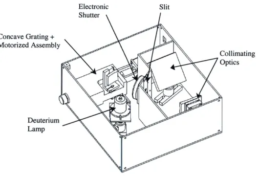
These UV light systems cannot be used in our application since they do not fulfill some important specifications. The spectroscopic system is large and has a small output beam, whereas the transilluminator has a fixed wavelength and a non-uniform output. Therefore, the design of a custom variable light source that meets the aforementioned specification is needed. Figure 3.8 shows a drawing of the proposed light source.
Electronic Concave Motorize( Slit Shutter Grating + d Assembly Collimating Optics Deuterium Lamp
Figure 3.8: Proposed light source.
The variable light source is composed of three main components: the lamp, the filtering system (concave grating and motorized system), and the optics to focus and collimate the light.
3.4.3 Lamp Choice
A lamp that can provide a stable continuous output in the UV range is needed for the light
system. There are four types of UV lamps available: deuterium, xenon, xenon-mercury, and hollow cathode. Table 3.1 shows a summary of their properties. The deuterium lamp is the ideal choice for the desired application since it provides a highly stable continuous ultraviolet output with little visible and infrared emission.
Lamp Type Wavelength Spectrum Stability Price
(nm)
(% p-p)
Deuterium (L2D2) 185 - 400 Continuous broad 0.05 Cheapest
Xenon 185 - 2000 Continuous broad 1 Expensive
Xenon-mercury 185 - 2000 Continuous broad 2 Expensive
Hollow cathode 193 - 852 Line N/A N/A
Table 3.1: Different available UV lamps. (Courtesy of Hamamatsu Inc)
A L2D2 deuterium lamp and a C4545 power supply from Hamamatsu are used. L2D2 lamps
have a lifetime twice as long as conventional deuterium lamps, around 2000 hours. Moreover they are 1.3 times brighter and have a higher stability and lower drift as seen in Figure 3.9.
Fluctuation:0.05%p-p
CONVENTIONAL TYPEr
TIME 10SadIV.)
Figure 3.9: Comparison of lamp output stability (Courtesy of Hamamatsu Inc)
There are a variety of lamp sizes and shapes. Types L6311-50 (0.5mm aperture) and
L6312-50 (1mm aperture) are selected because they have the smallest size and are already mounted to a
base. This facilitates mounting and more importantly alignment. The 0.5mm aperture has a high brightness arc, whereas the 1mm aperture provides a more uniform distribution. The selection between the two types is made through experiments.
To obtain the performances highlighted above, the lamp power supply needs to provide a constant current for the main power supply section and a constant voltage for the filament power supply. The Hamamatsu C4545 power supply is specifically designed for these lamps, and
therefore is used in the system. Technical information for these components is presented in Appendix C3.
To select the best lamp for our system, each was characterized by looking at its actual spectrum and its light distribution. Figure 3.10 shows the spectrum of the L6312 lamp taken using the spectroscopy system. L6311 spectrum is the same as the L6312 except for a slightly larger amplitude, therefore it is not shown.
10' Bulb L6312-50 (1 mm aperture), Intensity at 100mm
3 2 .5 - --- ---1 0.5 - -200 250 30 350 400 450 500 550 600 650 Wavelength (nm)
Figure 3.10: Spectrum of the L2D2 deuterium lamp using the CCD detector.
The spectrum shown in Figure 3.10 was obtained at a distance of 100mm directly in front of the lamp. It exhibits some variation from the spectrum advertised by Hamamatsu. The curve from 210-400nm should have a smooth decrease. The spectrum taken with the CCD camera in Figure 3.10 shows bumps around 240nm, 300nm, and 370nm. The CCD detector causes these bumps. The CCD quantum efficiency is wavelength dependent. As seen in Figure 2.5, the QE curve has sharp variations in the UV region. The bump locations correlate perfectly with the sharp changes in the QE of the CCD. One should be aware that each optical element that interacts with the light changes the shape of the spectrum because of its wavelength dependent quantum efficiency. Therefore, these components should be chosen to ensure a uniform intensity distribution in the wavelength range of interest (200-400nm in the proposed design).
Distance 1000 100 50 0,00 a) -10* LightFxdfbe
Deuterium lamp output optic detector
is rotated around its center axis
Spectrometer
x 10" Bulb 6312-50 (1 mm aperture) Intensity at Angle (-15 to 0 degrees) 3
angles -12.5 to 0 degrees are close to each others
100
1.5
-1 Increasing
(-15 to 0 degrees)
Step sire: 2.5 degree 0.5
200 250 300 350 400 450 500 550 600 650
Wavelength (nm)
x 104 Bulb 6312-50 (1 mm aperture) Intensity at Angle (0 to 15 degrees)
3 1
2.5
Increasing 2 (0 tQ 15 degrees)
Step size: 2.5 degrees
S1 .5 - - -- - - -
-C)
01
200 250 300 350 400 450 500 550 600 650
Next, the light distribution of the bulb was determined by measuring the intensity variation at different angles relative to the lamp center as shown in Figure 3.1 la. The spectrum of the lamp was recorded every 2.5 degrees from -15 to 15 degrees and analyzed using Matlab.
From the results shown in Figure 3.11 (b) and (c), two observations can be made. First, the separation distance between each spectra is proportional to their intensity, and this ratio does not change with different wavelengths. Therefore, in this case, the intensity distribution is wavelength independent. Second, the spectra from -12.5 to 0 degrees are close to each other. As the angle is increased outside this region, the intensity decreases quickly. Hence, there exist a range of angles where the light intensity is more uniform thereby exhibiting Gaussian distribution. However, this range is not centered at the origin (0-degree). To check this assumption, the intensity at the specific wavelength of 254nm versus the angle is plotted and presented in Figure 3.12.
x 104 Bulb 6312-50 (1 mm aperture) Intensity versus Angle
+ + ± band 15 d --... ... . -.. -.. Iw + ' + rdth grees - ... .. -A - .. ...-.. -15 -10 -5 0 5
Angle from certer(degrees)
.. ...
+
10 15 20
Figure 3.12: Lamp intensity at 254nm versus the angle.
As seen in Figure 3.12, the maximum intensity is at -5 degrees, therefore in the system, the lamp should be rotated counterclockwise 5 degrees. Also, a section of 15 degrees centered at -5 degrees will ensure 95% uniformity of the lamp output.
1.8
1.6
+ 100 mm away from bulb
95% . .~ ...- 90% :... ... 1.4 k-.. .... E ' AI C4 I 0.8 V.0 --20 I 2 --.. .. .. -. .. -. ... .. ... ... ...
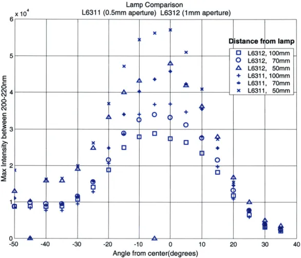
Figure 3.13 shows the comparison between the two different lamps. Using the same set-up as Figure 3.11a, the maximum intensity between 200nm and 220nm versus the angle was recorded for each lamp at three different distances (50mm, 70mm, and 100mm).
E a 0 e~j 0 0 C Z% x 10 -50 Lamp Comparison L6311 (0.5mm aperture) L6312 (1mm aperture) -40 -30 -20 -10 0 10 20 30 40
Angle from center(degrees)
Figure 3.13: Lamp intensity versus the angle for each bulb.
This graph shows that both lamps have an off center peak around -5 degrees. As expected, the 0.5mm aperture lamp is brighter and has a sharper peak than its 1mm counterpart. This means that the 0.5mm aperture lamp should be used if light throughput is important, whereas the 1mm aperture should be used to provide a more uniform beam when using the 15-degree bandwidth. For the first prototype, the 1mm aperture is used since beam uniformity is more important for molecule visualization.
Distance flrom lamp
5 X E3 L6312, 100mm 0 L6312, 70mm A L6312, 50mm + L6311, 100mm A -6 L6311, 70mm 4 __ __ _ x L6311, 50mm 0 + A 0 A 0 X0 A 00 + 1 -A _
_-A-3.4.4 Different Approaches to Filtering
The deuterium lamp that was selected emits a broadband spectrum. Its output needs to be filtered so that the user can select a specific wavelength. Two different filtering methods, rotating filter wheel and diffraction grating, were identified and will now be presented.
Filter wheels are commonly used to select a specific wavelength beam. Band-pass filters that only transmit light of a specific wavelength are attached to a wheel as seen in Figure 3.14. The wheel is rotated about "axis 1" to bring the desired filter in the light path.
Lens Lens Mirror 0 Deuterium Lamp Axis 1 185nm-400nm A 2xis Filter Wheel
Figure 3.14: Filter wheel approach.
Band-pass filters are simpler in design and have a higher throughput than most other filtering methods. However, this design's disadvantage is that only a finite number of wavelengths can be selected. One way to expand the application of this design is by taking advantage of the fact that the transmitted wavelength through a filter varies with the incidence angle of the light. Therefore by rotating the filter wheel around "axis 2", the transmitted wavelength shifts towards shorter wavelengths with increasing angle. The relation between the angle and the transmitted wavelength is [10]:
A = AO 1 -n- sin20 (3.1)
Where
A is the wavelength at angle of incidence,
Xo is the wavelength at normal incidence,
O is the angle of incidence,
no is the refractive index of external medium, neff is the effective refractive index of filter.
Variation of wavelength with incident angle 160 --- - - - --140 -+- 260rn 134.39 E 120 -- -- 2350nm 100 C 80 60 - "I1go 40 3524 20 3.97 1.-0 14.87 0 5 10 15 20 25 30 35 Degrees
Figure 3.15: Variation of wavelength with incidence angle.
Figure 3.15 shows the variation of wavelength with the incidence angle for the UV region (260nm) and for the IR region (2350nm). The transmitted light intensity decreases sharply after approximately 25 degrees; therefore the maximum variation in the UV region is only 10nm. This means that about 20 filters would be required to cover the 200-400nm range desired. In the infrared region however, a variation of 95nm is possible at 25 degrees. This difference between the two regions of the light spectrum is because the variation at a given angle is proportional to the wavelength. In summary, this method could only be applied to an application in the infrared but not in the ultraviolet range. Another method is therefore necessary.
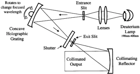
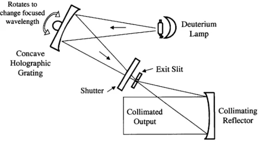
The second filtering method consists of using a diffraction grating to spatially separate the light into its monochromatic components. A schematic of a possible design is shown in Figure 3.16.
Rotates to Entrance
change focused Slit
wavelength
Concave Lenses Deuterium
Holographic Lamp
Grating Exit Slit 190=-400=
Shutter
Collimated Collimating
Output Reflector
A brief overview of the diffraction grating concepts is presented below. For a detailed
explanation, one should consult appropriate literature such as reference [11].
A typical diffraction grating consists of a substrate with a large number of grooves
(>600lines/mm) ruled on its surface as seen in Figure 3.17. grating normal incident light 0 diffracted light diffracted 1lg light d
Figure 3.17: Diffraction grating [11]
The incident light on the grating surface is diffracted into discrete directions. The grating equation, which governs this diffraction, can be written as:
mX = d (sin a +sinfi) (3.2)
where
m is the order of diffraction (an integer), A is the wavelength,
d is the groove spacing, a is the incidence angle, ,8 is the diffraction angle.
A common application of diffraction grating consists of changing the wavelength by rotating
the grating about its axis, with the incidence and diffraction light direction remaining constant. The angles a and /8 change as the grating is rotated, but the difference between them remains constant. This angle is called the deviation angle, 2K:
2K = a -8 = constant. (3.3)
The grating equation can be rewritten as
mA = 2d cos K sin 0, (3.4)
where
Equation (3.4) is required to design the mount for the grating. It shows that the diffracted wavelength at the output slit is directly proportional to the sine of the angle
#,
which is the grating rotation angle. This relation is the basis for the grating driving mechanism seen in Figure 3.18.axis of grating rotation (out of page)
grating
screw
Figure 3.18: Grating driving mechanism. [111
The relation between the arm length L, the distance X, and the angle
#
is:sino =-. (3.6)
L
Finally, the grating equation can be written as
X
mA = 2d -cosK. (3.7)
L
Equation (3.7) shows that as the distance X increases, the diffracted wavelength A increases linearly with X.
It is important to note that more than one combination of m and A will satisfy the equality of Equation (3.7). For example both m=1, A=A and m=2, 2=2/2 are valid solutions. This means that at a given angle, there is overlapping of diffracted spectra as seen in Figure 3.19.
grating normal 0 incident light m = +2 300 200 100 nm nm nm in = +1 600 400 200 nm nm nn
![Figure 2.2: Instrumental set-up of a capillary electrophoresis system. [2]](https://thumb-eu.123doks.com/thumbv2/123doknet/14685825.560232/21.918.235.656.136.441/figure-instrumental-set-capillary-electrophoresis.webp)
![Figure 2.4: CCD based DNA detection in systems for electrophoresis gels. [9]](https://thumb-eu.123doks.com/thumbv2/123doknet/14685825.560232/24.918.222.649.146.501/figure-ccd-based-dna-detection-systems-electrophoresis-gels.webp)