DEVELOPMENT OF A NEW EQUATION OF STATE FOR WATER AND ITS APPLICATIONS - PARTS I & II
by
PYUNG-HUN ,?1ANG
B.S.,Seoul National University (1974)
SUBMITTED IN PARTIAL FULFILLMENT OF THE REQUIREMENTS OF THE
DEGREE OF
MASTER OF SCIENCE IN MECHANICAL ENGINEERING
at the
MASSACHUSETTS INSTITUTE OF TECHNOLOGY June 1984
Q) Pyung-Hun Chang 1984
The author hereby grants to M.I.T. permission to reproduce and to distribute copies of this f-hess document in whole or in part.
Signature of Author... ... ... ... Department of Mechanical Engineering
Fyruary, 1984 Certif i: * (A1 .. 0 6.. .-...-... 0* 0& 0 9 00 . ...0 00 00
William C. Unkel
A Thesis Supervisor
Accepted Dy....
Warren M. Rohsenow Chairman, Departmental Commitee on Graduate Studies
MASSACHUSETTS INSTlTTE OF TECHNOLOGY
JUL 1
7
1984 Archives
preface
The purpose of this study was to develop a simple equation of state in the form of a thermodynamic potential function to represent the right image of pure water substance, yielding accurate thermodynamic properties. The intended use of the equation was to apply to problems in the steam power plant engineering.
The first part of this study covers the development of a new equation of state, while the second part treats the application of the equation of state to two engineering problem.
The author would like to thank Professor Henry M. Paynter for providing the motivation and the initial guidance of the study. He thanks deeply Professor William Unkel for providing timely guidances and encouragement, essential to the completion of this study. The author also thanks Professor Derek Rowell for his valuable suggestions and
encouragement.
The author thanks his wife Minja for her exceptional patience and love, his two sons Chai and June for their
DEVELOPMENT OF A NEW EQUATION OF STATE FOR WATER AND ITS APPLICATIONS-PARTS I & II
BY
PYUNG-HUN CHANG
Submitted to the Department of Mechanical Engineering on February 5, 1984 in partial fulfillment of the requirements for the Degree of Master of Science in
Mechanical Engineering
ABSTRACT OF PART I
An equation of state for pure water was developed in the form of a thermodynamic potential function, the Massieu Potential Function (MPF). The goal was to provide computationally simple, but accurate, expression that can be applied to problems associated with steam turbine cycle calculations, especially in control systems.
A generalized potential function was formulated after examining several theoretical equations of state including the van der Waals(VDW) equation. The potential function for water was determined from this - generalized function by evaluating the accuracy as additional terms were added. Accuracy was defined in terms of agreement of the equation results with the saturation curve behavior of water.
The resulting potential function (or equation of state) consists of 4 parameters, has one more term than the VDW equation, yet gives much better accuracy. The accuracy of pressure calculated with the present equation of state, as compared to data in the Keenan-Keyes-Hill-Moore steam table, is: within 1 % deviation in the temperature range from 200 F to 1400 F, with the pressure range from 5 psia to more than 2000 psia in the superheated region; and within 9 % deviation in the pressure range from 1.5 psia to the critical point in the saturated region.
The main improvement in the accuracy in the saturated region might be made by allowing the variation of the parameter b with temperature, which could reshape the pressure-volume-temperature relationship in the saturated region. The accuracy in the superheated region might be improved by adding a few empirical terms in the form of MPF to correct the compressibility factor.
Thesis Supervisor: Dr. William C. Unkel Title: Associate Professor of Mechanical Engineering
CONTENT OF PART I Page Preface... Abstract... List Of Tables... List Of Figures... Chapter 1. Introduction... 1.1 Background... 1.2 Problem Statement... 1.3 Organization... Chapter 2. Historical Review
Of The Research 2.1 Historical Review... 2.1.1 Improvements To 2.1.2 Improvements To 2.1.3 Inclusion Of Ro And Direction. Repulsion Te Attraction T tational And. rm. erm &... Vibrational Term 2.1.4 Inclusion Of Polarity... Combination Of Improved Results... 2.2.1 LHW And Guggenheim Equations... 2.2.2 The Equation By Whiting et al.. 2.3 Requirements And Direction For...
The Research
2.3.1 Requirements... 2.3.2 Direction... 3. Procedures Of Development... Review
6f
Thermodynamical Relations. 3.1.1 Thermodynamical Relations... 3.1.2 Reduced Form Of...Thermodynamical Relations
3.1.3 The MPF In Reduced Form For.... Existing State Equations
3.1.4 Assessment Of Equations In... Terms Of Saturation Properties 3.1.5 Assessment In Terms Of...
Compressibility Factor ... 25 ... . . . 26 ... . . . 27 2.2 Chapter 3.1
3.2 Procedures Of The Proposed Improvement. 3.2.1 The Formulation Of A...
Generalized MPF
3.2.2 Procedures Of Selection Of... Parameter
Chapter 4. Results And Discussions... 4.1 Results... 4.1.1 The Resulting Equation Of State.... 4.1.2 The OTher Parameters 'a' and 'b'... 4.1.3 Comparison Of The...
Compressibility Factor
4.1.4 Techniques To Improve The Agreement Of Predicted Compressibility
4.2 Discussions... -... ... Chapter 5. Conclusions And Recommendations...
5.1 Conclusions... 5.2 Recommendations... Bibliography... Appendix A. An Algorithm For The Computation...
Of Saturation Data 31 ... . . . 33 35 35 35 36 40 ... . . . 43 ... 44 .... .... .... 46 ... . 46 47 ...-.- -- 48 .... ... 49
List Of Tables
Table Page
1 Comparison Of The Three Equations With Experimental 18 Data
2 Comparison Of Saturation Data: Water, The Present 37 Result And The van der Waals Equation
3 Parameter Values Of The Present Equation Of State 39 4 Comparison Of The Compressibility Factor: Water And 40
The Present Result
5 Comparison Of Second Virials: Water And The-Present 43 Result
List Of Figures
Figure Page
1 Comparison Of Saturation Curves: Water, The van der 28 Waals(VDW) And Longuet-Higgins And Widom's Equations
2 Schematic Diagram Of The Second Virial Coefficient 30 3 Comparison Of Saturation Data: Water, The Present 38
Result And The VDW Equation - P vs. T
4 Comparison Of Saturation Data: Water, The Present 38 Result And The VDW Equation - P vs. V
5a Comparison Of Second Virial Coefficients In Linear 42 Scale: Water And The Present Result
5b Comparison Of Second Virial Coefficients In Log. 42 Scale: Water And The Present Result
DEVELOPMENT OF A NEW EQUATION OF STATE FOR WATER AND ITS APPLICATIONS
PART I
CHAPTER 1
INTRODUCTION
1.1 BACKGROUND
Quantitative calculations in the design and simulations of the steam power plants require reliable and computationally economical estimates of thermodynamic properties.. To obtain such properties, equations of state for water are required. Equations of state for fluids can be broadly classified into three categories: empirical, semiempirical and theoretical. Simple table lookup procedures or adjustment fit fall into the class of empirical, while those correlations where the basic form is defined on theoretical grounds but where the coefficients are 'fit' to the data are termed semi-empirical equations.
Since extensive experimental measurements of thermodynamic pro-perties are available for water, there exist many different empirical equations of state with a very large number of adjustable parameters that have essentially no physical significance. Among these are the 1967 IFC Formulation for Industrial Use and the 1968 IFC Formulation
for Scientific and General Use, both of which are based on the International Skeleton Table of 1963.[1] The former consists of about 150 numerical constants and the latter about 300 constants. These two IFC formulations have crucial weakness in that the range of state is split up into 6 sub-regions, each of which has different sub-formulation. Since the formulation is a curve fit of each property rather than a fit to a thermodynamic potential function like the Helmholtz free energy, thermodynamic consistency in each sub-region is not maintained nor is continuity enforced at their boundaries. The equation by Keenan, Keyes, Hill and Moore(KKHM) uses a single fundamental function with 59 constants.[2-j The fundamental function of the KKHM equation is the Helmholtz free energy as a function of temperature and specific volume, from which all the other steam properties can be derived. All the properties derived in this way are thermodynamically consistent with each other and continuous in the prescribed region. Nonetheless the larger number of constants of the KKHM equation is still disadvantageous for the computational efficiency. These totally empirical equations of state are quite accurate in making interpolative calculations of properties. For example, their accuracies are typically 0.01%. However, owing to larger number of constants, more than 90% of the CPU time is known to be spent in evaluating steam properties, when these types of state equations are used, in typical simulations of transient or steady state behavior of steam power plant components.[3] This computational disadvantage is one reason to develop theoretical or semi-empirical expressions.
A few theoretical equations exist for such simple substances such as argon or methane, although considerable mathematical and conceptual difficulties delay the rigorous theory of dense fluid. Among them is
an equation proposed by Longuet-Higgins and Widom.[4] However, the complicated nature of the water molecule (such as strong polarity) makes it difficult to derive a totally theoretical equation of state. Even semiempirical equations are quite rare. One of such equations is by Whiting and Prausnitz.[5] Another is proposed by Haar and
well known physical concepts suggested by van der Waals [VDW] over 100 years ago. The VDW equation can be considered to consist of two terms: the first one is repulsion term and the other attraction term. The equation by Whiting et al uses the Carnahan and Starling equation[7] as the repulsion term and the molecular dynamic results of Alder[81 as the attraction term. In addition, the equation uses the simplfied assumtion proposed by Prigogine[9], i.e. that at high densities, all density-dependent rotations and vibrations can be treated as equivalent translational degree of freedom. The result of the approach of Whiting has 10 coefficients and 4 adjustable parameters. However, in spite of rather sophisticated theoretical ideas, the accuracy is not good. On the other hand, the equation by Haar et al is composed of a reference function with some theoretical basis and a purely empirical function. This reference function is an updated VDW equation which is modified in part with theoretical basis and in part empirically so that it may represent the thermodynamic behavior quantitatively at high temperatures and elsewhere at high densities.
The motivation for this study, under the direction of Professor H.M. Paynter, came from the desire to find an equation which is simpler but more accurate than those available. Thus, in engineering calculations,good accuracy could be obtained with reasonable computational expense.
1.2 PROBLEM STATEMENT
The problem investigated in this study is to construct a potential function such as the Massieu potential or Helmholtz free energy from which all thermodynamic property can be derived. Like the forementioned semi-empirical equation, the starting point is the VDW equation. The immediate objective is to improve the VDW equation by simple theoretically or empirically base terms. More specifically, the objective is to find a better functional structure as well as
parameter values, so as to represent the right image of pure water ,yielding accurate thermodynamic properties with a simpler functional form for efficient calculations.
1.3 ORGANIZATION
In Chapter 2, a detailed historical background for the equation of water is given. This is followed by the direction and criteria for the development of the equation of state. Procedures of the development of the equation are presented in Chapter 3. Thermodynamical relations with regard to the Massieu Potential
Function is briefly reviewed. Main procedures of the thesis are presented here. Chapter 4 contains results and discussions, and conclusions and recommendations are presented in Chapter 5.
CHAPTER 2
HISTORICAL REVIEW AND DIRECTON OF RESEARCH
In this chapter, various fluid models are introduced and reviewed so that a rational direction for a derivation of new equation of state might be found. In addition, the criteria which appear to be crucial
for the development will be presented.
2.1 HISTORICAL REVIEW
The equation originally proposed by van der Waals[10]
(P+a/v 2)(v-b)=RT (2.1)
can be rewritten as
where P is pressure, T is temperature, v is specific volume, b accounts for the excluded volume by molecules and 'a' is the constant which represents the long range attraction force. The first term in Eq.(2.2) may be interpreted as the intermolecular repulsion term Pr, the second term as the attraction term Pa respectively. In other words, the pressure is composed of
- P = Pr + Pa. (2.3)
The VDW equation gives a moderately good description of P-V-T behavior in the gas phase where the excluded volume of each molecule does not overlap. However it gives only a qualitative description in the liquid phase since the volume v in the liquid phase is found experimentally to be considerably less than b. The improvements to the VDW equation can be either in improved repulsion or in improved attraction term.
2.1.1 Improvements To Repulsion Term
Several attempts have been made to improve the repulsion term of the VDW equation by adopting the model of hard-sphere molecules i.e. molecules where the two body potential function ] is given by
I'(r)= 0 , for r <a
I'(r)= oo, for r > (2.4)
where r is radial distance and a is the radius of hard core of each molecule. [11] For such molecules, Pa = 0. Sophisticated mathematical techniques have been applied to the model, in addition to a variety of assumptions concerning the properties of the radial distribution function.[Ill] Various assumptions and techniques are well reviewed in Reference 11. Relatively succesful equations of state include one by Percus-Yevic-Frisch(PYF) equation and another by
Carnahan and Starling(CS). These equations are similar with the PYF equation being
2 3
P =[(1+y+y )/(1-y) }( RT/v) (2.5)
and the CS being
P
~
23 3P =[(l+y+y -y)/(1-y) }(RT/v) (2.6)
where y=b/(4v). These equations give the functional results for compressibility factor which agree well with the theoretical results by Alder. Alder solved the equations of motion of small assemblies (tens or hundreds) of hard-sphere molecules with a computer and generated the properties of this system. The properties thus obtained can be considered as those of an 'ideal liquid' comparable with the perfect gas[12}, even though they may not be compared with experimental data directly, because the assumption of hard-sphere model in Eq.(2.4) is an over-simplified description of behavior of
real molecules.
2.1.2 Improvements To The Attraction Term
On the other hand, as an improvement over the attraction term, Pa, the molecular dynamic results of Alder show that the constant 'a' in the attraction term of the VDW equation actually depends on temperature and density. By using the square well potential as the two-body potential function, he derived the constant 'a' as
4 M M-1 n-1
a = -R(e.q/k)(r.vo)Y I (m.Ap/v~ )(1/T
)
(2.7) n=1 m=1where R is the gas constant,e.q is characteristic energy per molecule, k is the Boltzmann constant and r is number of segments per molecule
with v=v/(r.vo), where vo is the close-packed volume.
2.1.3 Inclusion Of Rotational And Vibrational Term
In addition to translation, larger molecules can exercise rotational and vibrational motions. Beret and Prausnitz[1
5
1 expressed the pressure with three terms, that is
P = Pr + Pa + Prv (2.8)
where Prv is the term to account for the rotation and vibration. Since it is difficult to construct a satisfying theory for evaluate Prv, Prigogine has suggested a simplifying assumption that all density-dependent degree of freedom may be considered to be equivalent translational degrees of freedom with
Prv = (c-1)Pr (2.9)
where c is an adjustable parameter for each substance. For fluids with larger molecules, c will be larger than 1, while for simple fluid with no rotation and vibration, c=1.
2.1.4 Inclusion Of Polarity
To account for orientational forces of strongly polar substance such as water, Gmehling et al[13] proposed an assumption that the substance is an equivalent mixture of monomers and dimers at chemical equilibrium and that the thermodynamic properties can be represented by the hypothetical mixture. The extent of dimerization is given by an equilibrium constant, K
2 2
K = (CD M P) (2.10)
where . is the true mole fraction,
#
is the fugacity coefficient, P is the total pressure and subscripts M and D denote monomer and dimer respectively. The Eq.(2.10) is used to find the mole fractions. Once the fractions are known, a set of constants are given as a function of composition by mixing rule, which is described more in detail-in the appendix of Reference 5.2.2 COMBINATIONS OF IMPROVED RESULTS
The more successful improvements over the VDW equation include imporvements to both the attraction and repulsion terms. They can be considered in two classes.
2.2.1 LHW And Guggenheim Equations
Longuet-Higgins and Widom(LKW)[4] combined the repulsion term given by the PYF equation, Eq.(2.5) with the VDW expression for Pa in Eq.(2.2). Both of the terms have physical meanings. Guggenheim(14) combined the same attraction term in Eq.(2.2) with an empirical repulsion term
Pr = [1/(1-y)4 RT/v (2.11)
which is algebraically simpler than the PYF equation but leads to almost identical predictions. The equations are
[ 2+~ 3 2 (.2
P = [(1+y+y )/(1-y) ] RT/v - a/v ;LHW (2.12)
Both of them are have two free parameters a, b (or bo). excluded volume b is determined either by using the relation
Usually,
3
b = 2 7rNau /3
where Na is the Avogadro's number and a/2 is radius of hard core of each molecule , or by matching a point of interest such as critical point.- The attraction parameter 'a' is evaluated primarily by matching points of interest. Guggenheim compared the accuracies of VDW, LHW and Guggenheim(G) with experimental data on argon. The comparison is given in Table 1 [14],where c denotes critical condition, t the triple point, Tb the Boyle temperature and vi the specific liquid volume at the triple point.
Table 1. Comparison of The Three Equations with Experimental Data of Argon
LHW 0.36 2.68 0.302 0.535 Guggenheim 0.36 2.72 0.303 0.528 Experiments 0.29 2.73 0.374 0.557
2.2.2 The Equation By Whiting Et Al
Whiting and Prausnitz used the expression Starling for the repulsion term, Alder's results term and adopt Prigogine's assumption for the vibrational term to represent water. In the
of Carnahan and for the attraction rotational and form of partition VDW (Pv/RT)c Tb
/
Tc vi/
vc Tt/
Tc 0.375 3.375 0.377 0.350function
Q,
their ruslt is expressed asN Nc Nc N
Q = (1/N!)(V/A ) (Vf/V).exp[-5 /2kT].(q)int (2.14)
where N is the number of molecules in total volume at temperature T, Vf is the free volume, k is the Boltzmann constantA is the de Broglie wavelength, and D/2 is the potential energy per molecule and where c is the parameter to account for the rotation and vibration as
introduced in Section 2.1.3. The free volume
2 2. ln (Vf/V) = [3( r/v) - 4( r/v)]/ (1- r/ v) (2.15) where T = 1
/18
and 2 5 n m /2kT = Y. (Ann-/T V)
(2.16) n=1 m=1with T = T/(eq/ck) and all other variables are defined in Eq.(2.7). By assuming that real water can be represented by a hypothetical mixture of monomers and dimers, Whiting and Prausnitz account for orientational forces due to the strong polar nature of water. This term is expressed in the form of the partition function
Q
of mixture and the details are shown in Appendix A of Reference 5. The resulting equation of state has in principle 8 adjustable parameters to fit experimental data. However, by using a set of simplifying assumptions, they reduced the number of parameters to 4. The final parameters are Tm*, Vm*, AHo and ASo, where the superscript * denotes characteristic values, subscript m represents monomers, and where AHo and ASo are the enthalpy and entropy of dimerization in the saturated state respectively. Incidentally, the parameters 'a' and 'b' are included in Vm*, and 'Anm' respectively.For water, the equation gives the accuracy of within: 4.5% and 4.6% deviations of saturated liquid volumes and vapor volumes from the triple point to just below the critical point; 2.2% deviation of superheated volume; 0.1% deviation of saturated pressure, up to a
temperature of about 1400F and a pressure of about 14000psia.
2.3 REQUIREMENTS AND DIRECTIONS FOR THE RESEARCH
2.3.1 Requirements
Before the detailed direction of the research is discussed, it seems proper to specify the requirements for the further development of equation of state, primarily from the previous review of historical backgrounds,but also partially from consideration of the intended use of the equation.
The criteria according to which the results must be judged may be stated as follows:
1) The properties generated by the resulting equation of state must be as accurate as possible for its level of complexity.
2) The equation of state must be as simple as possible for the economy of computation.
3) The equation of state should be able to acccurately
represent water in the two phase region, since the intended use of the equation is mostly to anyalyze performances of steam turbine cycles.
4) It is preferred that all terms in the equation have identifiable physical significance.
5) The properties should be generated to be selfconsistent throughout the desired interval.
2.3.2 Direction
It was shown in Eq.(2.9) that the rotational and vibrational term became an additional repulsion term. Accordingly, Eq.(2.8) reduces to Eq.(2.3) with a resulting modified repulsion term. In addtion, it is obvious that the attraction term a(v,T) in Eq.(2.7) makes the equation of state much more complicated than constant 'a'. Thus, it appears to be worth attempting:
1) to improve the accuracy of equation of state by modifying the repulsion term; and
2) to improve the simplicity of the equation by keeping 'a' in the attraction term constant.
The improvement on the repulsion term would be made by modifying the repulsion terms introduced in Section 2.1 with empirical terms (even though they may not be clearly correlated to microscopic behavior of molecules).
Since thermodynamic properties generated by a thermodynamic potential function satisfy the Maxwell's relations, they are consistent with each other. Additionally, it can give smooth and continpus transition from one state to another as well as from one phase to another phase. Therefore, it is much more desirable to construct the equation of state in the form of thermodynamic potential function such as the Helmholtz free energy or alternatively the Massieu Potential Function(MPF). According to these considerations, the direction may be stated as:
---To construct an equation of state in the form of thermodynamic potential by making improvement on the repulsion terms in a macroscopic way.
---CHAPTER 3
PROCEDURES OF DEVELOPMENT
In this chapter, thermodynamical relations regarding to the Massieu Potential Function(MPF) are briefly reviewed. Then they are expressed in terms of a set of reduced properties. After various MPF are assessed, the procedure of proposed improvement is given.
3.1.1 Thermodynamical Relations
The Massieu Potential Function(MPF) J, which has been named after its originator, is defined as
J = S - U/T - -F/T (3.la)
where S, U, F and T are respectively entropy, internal energy, Helmholtz free energy and absolute temperature. The negative Massieu
function J is then
J = - J = F/T (3.1b)
By using the well known relation
P = -( aF/ aV)T (3.2)
and Eq.(3.1), where P is pressure and V is total volume, we obtain for temperature and internal energy the expressions
(3.3)
P = (aJ/ a V)T
7-P =P (aJ/8P) T and
U = (aJ/ar ) (3.4)
where T is the inverse of temperature and p is the density
respectively. With Eq.(3.la), the remaining expressions properties can be expressed as
S = U/T - J and
G = H-TS = JT + PV
where G and H are te Gibbs free energy and enthalpy respectively. for
(3.5)
The negative MPF then can be used to completely construct the thermodynamic properties of the material.
3.1.2 Reduced Form Of The Thermodynamical Relations
The negative MPF for the VDW equation can be easily derived as
J/m = R ln b/(v-b) - a/v/T + J,/m , (3.7)
where the first term on the right hand side can be interpreted as repulsion term, the second as attraction term and the third term Jr/M as a part of the PF which is function of temperature only, with m and v, mass and specif ic volume of the material.
If the MPF and corresponding state equations are expressed in reduced forms, not only they become more compact, but also comparisons between different terms are easier. The reduced properties are defined as y bo/v; (3.8a) 2 P (bo /a)P; (3.8b) = (a/R bo)/T; (3.8c) J (J/m)R; (3.9a) J'r (JT /m)R ; (3. 9b) and JyA J - JT (3.9c)
where Jy is a part of the reduced MPF excluding J and with bo the actual volume of one mole of molecules, given as
bo = Na ( 7r /6)a = b/4
where a/2 is radius of hard core, Na the Avogadro's number and b the excluded volume in the VDW equation. The corresponding thermodynamical relations for the reduced properties become
P = y (aj/ ay)T u = (aJ/ar)y G = J + P/y s u T - J h u + P/y (3.10) (3.11) (3.12) (3,13) (3.13)
3.1.3 The MPF In Reduced Form For Existing State Equations
The MPF's of the VDW, LHW, Guggenheim(G) and CS are
(Jy) = In VDW (4y)- ln(1-4y) -(Jy) = in y - ln(1-y) yHW (Jy) = in y - ln(1-y)
yr
+ (3/2)(1-y) (3.16) (1-y7 + -2 + (1/2)(1-y) + + (1/3)(1-y) (3.17) and 25 (3.15) -- YT +(Jy) = ln y
CS
The similarities and differences of displayed. The resulting
pressure-volume-temperature become -1 + 2(1-y) + + the relationships expressions (3.18) are clearly f or the - y 3
[y(1+y+y )/(1-y) I/T - y 2 (3.19) 2. (3.20) P P
~-CS
4 =[y/(1-y) ]/T 2 -y - [y(1+y+y2-y3)/(1y)3]/(3.21)
(3.22)
3.1.4 Assessment Of Equations In Terms Of Saturation Properties
One way to assess the accuracy of the formulations is to compare the predicted and measured saturation properties. The thermodynamical relations in saturation states are given as
Tf = Tg P(vf,Tf) = P(vg,Tg) G(vf,Tf) = G(vg,Tg) (3.23a) (3.23b) (3.23c)
where f and g designate saturated liquid and vapor. For the reduced variables defined in Eqs.(3.8), the saturated expressions become
(3,24a) .rf = g P = VDW P = ~LHW and and [y/(1-4y)]/T
P(yf,Tf) = P(yg,rg) (3.24b) and
G(yf,rf) = G(yg,rg) (3.24c)
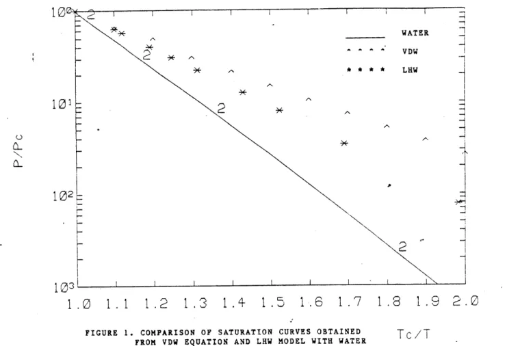
Eqs.(3.23a)-(3.23c) with Eqs.(3.12),(3.19),(3.20) and (3.21) yield the saturation properties. The saturation curves of the VDW, LHW and water are compared in Figure 1 in reduced coordinates P/Pc and T/Tc where the subscript c denotes critical condition. In these coordinates, saturation properties are independent of the parameters 'a' and 'b'. As can be seen, the equation suggested by LHW improves the agreement considerably, even though there is still significant mismatch. This may be viewed as a positive aspect. That is, since the Eq.(3.16) gives better saturation curve than Eq.(3.15) by using one more term, it may be probable that a still better saturation curve might be obtained with a relatively simple equation of state.
3.1.5 Assessment In Terms Of Compressibility Factor
From Eqs.(3.8a),(3.8b) and (3.8c) it can be shown that the compressibility factor Z is
Z = Pv/RT = P r /y (3.25)
The corresponding expressions for the compressibility factors of the VDW, LHW and Guggenheim equations are
Z = 1/(1-4y) - y r (3.26a) VDW Z = (1+y+y )/(1-y - y r (3.26b) LHW ~ and z = 1/(1-y) - y T (3.26c) G
101
103
1. 1
1 .0
1 .1
FIGURE 1. COMPARISON OF SATURATION CURVES OBTAINED FROM VDW EQUATION AND LHW MODEL WITH WATER
1.2
1.3
1.1-
1.
1.6
1.'7 1.8 1.9
2.0
Tc/T
Each expression may be expanded in power series by using the relation
1/(1-x) = 1 + x2+ X3+ x4+ ... ; ixi < 1
The series expansions of the three equations are 2
Z 1 + (4- T)y + 16y +... (3.27a) VDW 2 Z 1 + (4- T)y + 1Oy +... (3.27b) LW and 2 Z G = 1 + (4- r)y + 10y +... , (3.27c)
Since the virial coefficients B, C, D ... are defined as
2 3
Z - 1 = B/v + C/v + D/v +...
it can be shown from Eqs.(3.8a),(3.8c) and Eqs.(3.27) that the second virial coefficients, B of all the three equations are linear functions
of inverse temperature, 1/T as
B = 4bo - (a/R)/T (3.28)
The second virial coefficient depends on values of 'a' and bo, which are determined, as described in Section 2.2.1, either by matching a point of interest or by theoretical calculations.
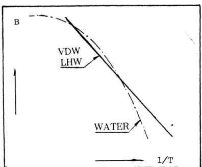
Measurements of water properties show that second virial coefficient of water is a complicated function of 1/T.[2] The second virial coefficient of the three equations in Eq.(3.28) is compared with water schematically in Figure 2. The comparison shows that Eq.(3.28) gives poor accuracy, especially in low temperature range. In fact, this aspect has been regarded as an intrinsic deficiency of the VDW-type equations in predicting the compressibility factor.
-. 1/T
FIGURE 2. SCHEMATIC DIAGRAM OF THE
SECOND VIRIAL COEFFICIENT
repulsion term with 'a' in the attraction term kept constant, the second virial has the same functional form as Eq.(3.28). Thus, the intended equation of state will have more or less the same deficiency in predicting the compressibility factor as the three discussed above. On the other hand, a significant mismatch in saturation data might be corrected without much sacrifice in the accuracy of compressibility factor. -This point will be discussed later in Section 4.1.3.
3.2 PROCEDURES OF THE PROPOSED IMPROVEMENT
3.2.1 The Formulation Of A Generalized MPF
Observation of functional forms of various MPF's in Eqs.(3.15),(3.16), (3.17) and (3.18) suggested to Professor H.M.Paynter a generalized repulsion term in MPF, which is expressed as
n i
J = ln y - Xln(1-y) + Y Mi/(1-y) -Y
i= 1
For example, this equation reduces to the repulsion term of the following special equations:
VDW: X=1; 'Li= 0 for all i
LHW: X=1; 42 =3/2; i = 0 for all other i
Guggenheim: A =1; P1 = 1; )2 =1/2; 1'3 =1/3; li=O for all other i
CS: A =0; /1 = 2; #2= 1 ; "i = 0 for all other i
Defining x=4y, P=16(bo /a)P and T =4(a/Rbh)/T, then the MPF of the VDW equation, Eq.(3.15) can be expressed as
Jy = in x - ln(1-x) - x (3.29a) (3,29a)
If it is noticed that the MPF
Jy = in y - ln(1-y) - y _ (3.29b)
and Eq.(3.29a) yield the identical saturation curves in the normalized coordinates P/Pc and Tc /T and that the saturation curve of Eq.(3.16) is closer to that of water than that of the VDW equation, effect of
1
'i/(1-y) in the repulsion term becomes clear. This effect is shown clearly in Figure 1. If the usual VDW attraction term is included, the general MPF becomes
n
Jy = In y - Xln(1-y) + : /li/(1-y) - y T (3.30) i=1
The corresponding equation of state for pressure and compressibility factor are
n
P = [y +xybl-y)2+ y Yi. P i/(1-y) ] - y (3.31)
i=1 n
Z = 1 +Xy/(1-y3 + y V i. Jli/(1-y - y T
(332)
i=1The theoretical basis of the MPF given by Eq.(3.30) may be open to serious questions, but its simplicity and descriptive ability make it attractive for further use, provided that it offers some advantages in trade-off for accuracy and computation time.
3.2.2 Procedures Of Selection Of Parameter
Eq.(3.30) has i+1 explicitly shown free paramenters. The approach is to choose values of i and, by use of the saturation data, to determine the best values of x and the i's. Comparison of the results for different values of i is then used to determine if there is a best value of i. The detailed procedures adopted may be summarized as follows:
1. Determine number of terms by examining the results for several values of i in Eq.(3.30).
2. Change step by step values of A and I1i's.
3. Obtain the critical point which is uniquely determined by the above set of parameters by solving the following equations
simultaneously for yc and Tc, and Pc accordingly,
(P/
ay),
=0;(9P/
ay
) =0where c designates the critical point.
4. Determine saturation curves by solving the following two equations for several T_'s betweenr = Tc and r =2 Tc,
P(yf,r) = P(yg,T); G(yf,r) = G(yg,r) (3.33)
where f, g designates saturated liquid and vapor respectively. Thus, obtain yf, yg and P for each T.
5. Compare these sets of saturation properties with those of water for several r using the quantitative measure I, as
n
2
I = X [ 1 - (P/Pc)m / (P/Pc)wI (3.34)
which represents deviations between the two, where m and w represent fluid model and water respectively.
6. Repeat the steps 2 to 6 until I becomes minimum.
For the procedures, an algorithm was implemented on the computer to solve the nonlinear equations
P(yfrf) = P(yg,rf)
G(yfTf) = G(yg,rf).
The program is listed in Appendix A. In addition, it may be emphasized that the above procedures were done independent of the values of the parameters a and b, since in the reduced form the
CHAPTER 4
RESULTS AND DISCUSSIONS
4.1 RESULTS
4.1.1 The Resulting Equation Of State
After executions of the procedures described in Section 3.2, it was found that neither increasing n in Eq.(3.30) to more than two, nor
chosing
X
other than unity improve the accuracy significantly, at least in terms of saturation properties. Thus any serious compromise between accuracy and simplicity is not required if the values of i=1, X=1 and sti=9 are selected. The MPF and the equation of state forpressure become as follows:
Jy = in y - ln(1-y) + 9/(1-y) - yr (4.1)
2 2 2
P = [y/(1-y) + 9y /(1-y) /r - y (4.2)
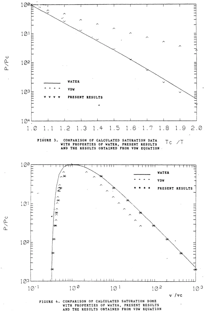
with those of VDW equation and water obtained from KKHM steam tables. The present results are presented and compared with VDW results of the saturation properties and water graphically in Figures 3 and 4. As can be seen, the present results accurately represents the pressure vs. temperature behavior in the two phase region and are somewhat better than the VDW equation in predicting the pressure-volume relationship in the saturated states.
Since the equation of state of P generated by the general form of MPF in Eq.(3.31) reduces to that of ideal gas as density P-(or y) become smaller, as should be the case, the behavior in this region is not shown in great detail here. The detailed discussion of compressibility and the second virial coefficient is given in Section 4.1.3.
4.1.2 The Other Parameters 'a' And 'b'
In principle, the excluded volume b in the VDW equation may be calculated from intermolecular motions. However, the large uncertainties in the knowledge of intermolecular motions of water make it more accurate to obtain b by fitting the P,V,T data at a proper point. of interest. Then the other constants a and R are determined simultaneously from Eqs.(3.8a) and (3.8b). It may be noted that since the three parameters a,b and R are interrelated to each other, they are determined only by one point of fitting. The resulting relations are b = 4bo bo; v y 2 a = bo (P/P) and R = T(a/bo)/T
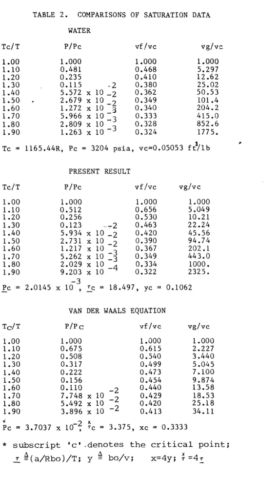
TABLE 2. COMPARISONS OF SATURATION DATA WATER P/Pc 1.000 0.481 0.235 0.115 -2 5.572 x 10 -2 2.679 x 10² 1.272 x 10 3 5.966 x 10 -3 2.809 x 10 1.263 x 10 vf /vc 1.000 0.468 0.410 0.380 0.362 0.349 0.340 0.333 0.328* 0.324 vg/ve 1.000 5.297 12.62 25.02 50.53 101.4 204.2 415.0 852.6 1775. Tc = 1165.44R, Pc = 3204 psia, vc=0.05053 ft/lb PRESENT RESULT Tc/T 1.00 1.10 1.20 1.30 1.40 1.50 1.60 1.70 1.80 1.90 Pc = 2.0145 P/Pc 1.000 0.512 0.256 0.123 5.934 2.731 1.217 5.262 2.029 9.203 -- 2 x 10 -2 x 10 -2 x 10 x 10 -3 x 10 x 10 -3 x 10 , Ic = 18.4 vf/vc 1.000 0.656 0.530 0.463 0.420 0.390 0.367 0.349 0.334 0.322 vg/vc 1.000 5.049 10.21 22.24 45.56 94.74 202.1 443.0 1000. 2325. 97, yc = 0.1062
VAN DER WAALS EQUATION
P/PC vf/vc 1.000 1.000 0.675 0.615 0.508 0.540 0.317 0.499 0.222 0.473 0.156 0.454 0.110 -2 0.440 7.748 x 10 2 0.429 5.492 x 10 2 0.420 3.896 x 10 -2 0.413 Pc = 3.7037 x 107 = 3.375, xc = 0.3333
* subscript 'c' .denotes the critical point; S= (a/Rbo)/T; y = bo/v; x=4y; - =4T
Tc/T 1.00 1.10 1.20 1.30 1.40 1.50 1.60 1.70 1.80 1.90 Tc/T 1.00 1.10 1.20 1.30 1.40 1.50 1.60 1.70 1.80 1.90 vg/vc 1.000 2.227 3.440 5.045 7.100 9.874 13.58 18.53 25.18 34.11
101
102
v v v v PRESENT RESULTS
1.0
1. 1
1.2
1.3 1.4
1.5 1.6 1.7
1.8 1.9 2.0
FIGURE 3. COMPARISON OF CALCULATED SATURATION DATA
Tc /1
WITH PROPERTIES OF WATER, PRESENT RESULTSAND THE RESULTS.OBTAINED FROM VDW EQUATION.
100
101
102
03-10~1
10
0
101
102
v /Vc FIGURE 4. COMPARISON OF CALCULATED SATURATION DOMEWITH PROPERTIES OF WATER, PRESENT RESULTS
AND THE RESULTS OBTAINED FROM VDW EQUATION
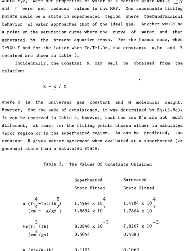
where P,v,T were set properties of water at a certain state while P,y and r were set reduced values in the MPF. One reasonable fitting points could be a state in superheated region where thermodynamical behavior of water approaches that of the ideal gas. Another would be a point on the saturation curve where the curve of water and that generated by the present equation cross. For the former case, when T=900 F and for the latter when Tc/T=1.56, the constants a,bo and R
obtained are shown in Table 3.
Incidentally, the constant R may well be obtained from the relation:
R = R / M
where R is the universal gas constant and M molecular weight. However, for the sake of consistency, it was determined by Eq.(3.8c). It can be observed in Table 3, however, that the two R's are not much different, at least for the fitting points chosen either in saturated vapor region or in the superheated region. As can be predicted, the constant R gives better agreement when evaluated at a superheated (or gaseous) state than a saturated state.
Table 3. The Values Of Constants Obtained
Superheated Saturated State Fitted State Fitted
4 2 4 4 a (ft -lbf/lb ) 1.4964 x 10 1.4184 x 10 4 2 7 7 (cm - g/gm ) 1.8854 x 10 1.7864 x 10 3 -3 -3 bo(ft /lb) 8.0848 x 10 7.8267 x 10
3
(cm /gm) 0.5044 0.4883 R (Btu/R-lb) 0.1103 0.1069 (J /K-gm) 4.622 4.476R = R / M = 4.615 (J / K-gm)
R = Universal gas constant; M = Molecular weight
4.1.3 Comparison Of The Compressibility Factor
The compressibility factor Z of the fluid model of Eq.(4.1) was calculated by using Eq.(3.32) and compared in Table 4 to the values for water as determined from KKHM steam table data.
Table 4. Comparison Of Compressibility Factor
Tr=T/Tc, yr=y/yc, y=b/4v
subscript c designates critical value
Tr 0.8 1.0 1.2 yr Zwater 0.012 0.065 0.010 0.051 0.104 0.423 0.008 0.085 0.366 0.816 0.9760 0.8366 0.9852 0.9266 0.8528 0.4994 0.9930 0.9375 0.7627 0.6000 Zmodel 0.9833 0.9103 0.9910 0.9545 0.9085 0.6593 0.9952 0.9527 0.8200 0.6940
coefficient B is derived for the present model. From Eq.(3.32), the compressibility Z is expressed as
2
Z = 1/(1-y) + 9y/(1-y) - y T (4.3)
As a power series, it is expressed as
Z = 1 + (10 - -)y + 19y +... (4.4)
From Eqs.(3.8a) and (3.8c), the second virial B becomes
B = 10bo - a/R/T (4.5)
By using the two sets of a,bo and R previously obtained, the corresponding second virial coefficients Bi and B2 obtained as 3 BI = 4.960 - 5.94617 (cm/g) 3 B2 = 4.700 - 5.81837 (cm/g) (4. 6a) (4.6b)
where B1 is for superheated water and B2 for saturated water, with
I A 1000/T K
The empirically derived expression of the second virial equation for water suggested, in Reference 2, by Keyes is
B = 2.0624 - 2.81204T 10 (cm /g)
- = 0.1008T / (1 + 0.03497
)
(4.7)
The three equations Eqs.(4.6a), (4.6b) and (4.7) are plotted in Figures 5a and 5b. Also values are tabulated in Table 5. Figure 5a shows a linear plot of B vs. c, while 5b shows a logarithmic plot. where
0
-10
--20
--30
-o2
-40
--50
-C
-60
-a
-'70
z
o
-80
-v9
-0
-100
0.5
1.0
1.5
2.0
2.5
3.0
TAU(1000/T K)
FIGURE 5a. COMPARISON OF THE SECOND VIRIAL COEFFICIENTSOF THE PRESENT RESULTS WITH WATER(LINEAR SCALE)
I A -WATER --- Bl(evaluated at the superheated state) * * * * B2(evaluated at the saturated state) I I I I
2.0
3.0
1.5TAUII100
K)
FIGURE 36. COMPARISON OF THE SECOND VIRIAL COEFFICIENTS OF THE PRESENT RESULTS WITH WATER
(LOGARITHMIC SCALE)
4.0
102L-101
100 C) 'K C) 02 -Ja
z
0 (9w
(:) 10n'O.5
0-.Table 5. (1000/T K) 1.00 1.40 1.80 2.20 2.60 3.00 3.40 3 COMPARISON OF SECOND VIRIAL B(cm 7g)
(B)water -1.21 -3.54 -7.18 -13.0 -22.1 -36.3 -58.0 B1 -0.986 -3.36 -5.74 -8.12 -10.5 -12.9 -15.3 B2 -1.12 -3.45 -5.77 -8.10 -10.4 -12.8 -15.1
The examination of the equation for the second virial-coefficient obtained from the fluid model shows that the two selection techniques for a and bo do not significantly affect the compressibility factor. As has been mentioned previously, the equation of state constructed has an inherent deficiency in the compressibility factor at low temperature. It is not so surprising that the mere constant 'a' and its linear representation, Eq.(4.5) have such a deficiency when compared to the empirical expression of Keyes.
4.1.4 Techniques To Compressibility
Improve The Agreement Of Predicted
One way to improve the compressibility factor would be to select a, b and R so that the deviation from measured data would be minimised for a certain temperature range. For instance, the linear regression
of the second virial between r =0.8 and 3.0 gives
which is substantially different to the results obtained by fitting parameter points as represented by Eqs.(4.6). This requires considerably different values of a, bo and R, which will cause undesirable new inaccuracies both at the saturation states and superheated states. Thus improvements should be to incorporate additional terms with a different functional form. For example, Whiting et al[5] modified by adding an empirical term in the form of the Helmholtz free energy which is
n
Fsv = (d/Tr ) exp (-Akp) , (4.8)
where Tr=T/Tc, d, n are constants which are determined from the second-virial-coefficient data, and A is a positive constant
for a better third virial coefficient. The correction term in Eq.(4.8) may be incorporated in Eq.(4.1) provided that it does not affect the computed saturation curve significantly. It may be worth attemptng for the future improvements of the equation of state in Eq.(4.1).
4.2 DISCUSSIONS
The new equation may be evaluated in terms of the criteria adopted, which were presented in Chapter 2.
Accuracy:
In the saturated region, for most of states from the critical point to about 1.5 atm., the agreement between calculated pressure and the KKHM steam table data is within 9%. In the superheated region, the agreements are within 1 %, with a temperature range from 200F to
Simplicity:
The equation has of four free parameters, which are a,bo,R and and has only one more term than the VDW equation. In addition, it
is easy to convert from one set of independent variables to another.
Saturation curve:
The present equation of state gives two phase region which is similar to water.
Physical Significance:
The theoretical basis of Eq.(3.30) and in particular the physical meaning of the term, 9/(1-y) are open to questions. It is difficult,
so far, to relate them to the knowledge of intermolecular motion.
CHAPTER 5
CONCLUSIONS AND RECOMMENDATIONS
5.1 CONCLUSIONS
A new equation of state for water in the form of Massieu Potential Function has been derived. The equation generates relatively accurate-properties, considering its simplicity. As shown in Figures 3 , 4 and Table 2, it gives much more accurate values than the VDW equation even though it has only one more term. While it may not be adequate for calculations which require high accuracy, it may be useful when employed either for the analysis of transient response in a steam turbine cycle, where the Runge-Kutta method or a related method of solving nonlinear differential equations require simplified equation of state for the evaluation of various steam property derivatives. Further it may be employed as a reference function[61 for the further refinements. Finally, the simple closed functional form this equation of state allows explicit evaluation of formal derivatives, and this may be an advantage over the empirical equations with complicated functional form or tabulated data.
5.2 RECOMMENDATIONS
In the previous development of equation of state, it has been assumed that the excluded volume b is constant. However, Haar et al[6] showed that b depends on temperature. They obtained the expression of the parameter b by fitting to the steam table data. It is given as
-3 -5 b(T) = b' + c ln T + d T + e T
where T = T/647.073 K and b',c,d and e are empirically determined values. Note that since the saturated curve was obtained without regard to b, varying b with T does not change the basic shape of the curve. It would be worth attempting to examine whether and how much a variable b(T) can improve P-V-T relationship.
Another improvement might be to find an approximate representation to Alder's attraction term as represented in Eq.(2.7) by some mathematical means like least square fittings.
As suggested in Section 4.1.4, an additional term might be used to improve the accuracy of the compressibility factor.
Bibliography
1. J.Straub, "Equilibrium Properties of Water Substance 1974-1979, Tasks and Activities of Working Group I," Water and Steam, Proc. of 9th Int. Conf. on Properties of Steam, edited by J.Straub and K.Scheffler.33
2. J.Keenan, F.Keyes, P.Hill and J.Moore, Steam Tables. John Wiley & Sons: N.Y.:1969
3. J.Campbell and R.Jenner, "Computational Steam/Water Property Routines," " Water and Steam, Proc. of 9th Int. Conf. on Properties of Steam, edited by J.Straub and K.Scheffler.142
4. H.Longuet-Higgins and B.Widom, "A Rigid Sphere Model for the Melting of Argon," Molecular Physics, 8: 549(1964)
5. W.Whiting and J.Prausnitz, "A New Equation of State for Fluid Water Based on Hard-sphere Peturbation Theory and Dimerization Equilibria,"" Water and Steam, Proc. of 9th Int. Conf. on Properties of Steam, edited by J.Straub and K.Scheffler.83
6. L.Haar, J.Gallagher and G.Kell, "Thermodynamic Properties for Fluid Water," " Water and Steam, Proc. of 9th Int. Conf. on Properties of Steam, edited by J.Straub and K.Scheffler.69
7. N.Carnahan and K.Starling, "Intermolecular Repulsion and The Equation of State for Fluids," Journal of AIchE, 18: 1184(1969)
8. B.Alder, D.Young and M.Mark, "Studies in Molecular Dynamics," Journal of Chemical Physics, 56: 3013(1972)
9. I.Prigogine, Molecular Theory of Solutions North Holland: Amsterdam, 1957
10.J.van der Waals,"Over de continueteit van den gas," (Dissertation, Leiden), 1873
11.H.Temperley, J.Rowlinson and G.Rushbrooke, Physics of Simple Liquids John Wiley & Sons Inc.:N.Y., 1968
12.B.Alder and T.Wainwright, " Studies in Molecular Dynamics II," Journal of Chemical Physics, 33: 1442(1960)
13.J.Gmehling, D.Liu and J.Prausnitz, "High Pressure Vagor-liquid Equilbria for Mixtures Containing One or More Polar Components
14.E.Guggenheim,"Variations on van der Waals' Equation of State for High Densities," Molecular Physics, 9(1965)43, 199
15.S.Beret and J.Prausnitz," Perturbed Hard-chain Theory. An Equation of State for Fluids Containing Small or Larger Molecules," Journal of AIchE, 18: 1125(1975)
Appendix A
In saturated states, the relations in Eq.(3.21) hold. If Eq.(3.31) is combined with Eq.(3.24b), then
2 2 2 2 2 2
yf -yg + A ( yf /qf - yg /qg ) + tI(yf /qf - yg /qg ) + + 2.L2 yf2 /qf - y2 /qg ) +
- r(yf - yg)
= 0 ~~ (A-i)
where q = 1-y. Then
= yf - yg + (yf2/qf - yg2/qg ) + (yf2/q2- yg q) + ... (A-2)
2 yg 2 yf Yg
Besides, From Eq.(3.12) and Eq.(3.21), we can derive
Jf - Jg + ' (Pf/yf - Pg/yg) = 0 (A-3)
If we combine Eq.(A-3) with Eqs.(3.30) and (3.31), then
ln yf/yg - kln qf/qg + pL(i/qf - I/qg) + p2 (i/qf - i/qg +
- r (yf - yg) + z (Pf/yf - Pg/yg) = 0 (A-4)
Then A 2 2
ln (yg/yf)(qf/qg) =I'l(1/qf - 1/qg) + lt2((L/qf -i/qg )+
+...- T (yf-yg) .. (A-5)
If the right-hand-side of Eq.(A-5) is set X, then Eq.(A-5) becomes
yg = yf (qf/qg) .exp(X) (A-6)
Both Eqs.(A-6) and (A-2) constitute the algorithm, which are now
_i yfi - ygi + x (yfi/qfi- ygi/qgi +.. (A-7)
yf - yg
yg i+1= yfi (qf /qgi) .exp(X
where i =1,2,.. . Incidentally, yg can be determined empirically, by yg 1= e qf 2
DEVELOPMENT OF A NEW EQUATION OF STATE FOR WATER AND ITS APPLICATIONS
PART II
ABSTRACT OF PART II
A new equation of state for pure water substance was applied to two problems associated with steam turbine cycle calculations, to evaluate the advantages of using the equation in the practical engineering situations. The evaluation was made primarily in terms of accuracy and computional speed, in comparison with another set of equations of state. This other set of equations follows a more standard development of equations of state for engineering calculations and, has 36 empirically determined coefficients for each combination of independent and dependent properties. In addition to the thermodynamic potential function describing the P-V-T behavior, it was necessary to determine the internal energy, enthalpy and entropy. This portion of the equation of state was constructed by incorporating the van der Waals expression and making a curve-fit to the Keenan- keyes-Hill-Moore(KKHM) steam table data.
The first problem was to determine thermodynamic states on the expansion line of steam partial loads. In this problem, the equations of state were used in a computer program, in conjunction with an empirical method by Spencer for evaluating the performance of steam turbines. The accuracy and computational speed with the two sets of
equations of state were measured and compared.
The second problem was to simulate the transient behavior of a small part of a heat exchanger typical of steam cycle systems. The equations of state and conservation laws of were applied to model the dynamic characteristics of the component. The transient response, when subjected to load changes, was simulated using the program package DYSYS as implemented on a VAX 11/780. Comparisons of accuracy and computational speed were made for this problem, again using the two sets of equations.
The results show the advantage of the equations of state developed in this study. Compared to the more typical approach, the accuracy is equivalent or slightly better and the computational time is reduced by a factor from 2 to 6, depending on the particular problem.
Further computational advantages might be achieved by algebraic manipulation of the simple equations of state in the present study. Considering that their simple closed forms allow formal derivatives, that most terms are physically identifiable, the equations might find their usefulness in applications where functional dependences are needed and where the empirical equations with complicated expression can not be used. The accuracy of the equation of state for the internal energy would be improved by adding terms similar to those of the KKHM formulation, which should give more accurate enthalpy and entropy.
CONTENT OF PART II
Abstract...-... List Of Tables... List Of Figures... chapter 1. Introduction.
Chapter 2. New Equations Energy, Entha Chapter 3. The Determina The Expansion 3.1 Introduction... 3.2 The Methods Of Performance Of 3.3 The Determinati 3.4 The Procedures 3.5 An Illustrative Chapter 4. The Applicati
OF A Heat- t 4.3 Chapter Page ... .. .51 55 Of State For The Inter
lpy And Entropy... tion Of
Line End Points...
Estimation Of Non.Rehea Steam Turbines... on Of The ELEP's... For The Computation ....
Example -... ... on To The Simulation
hanger... . -. --.-.
-Introduction... The Procedures Of Modell Simulation Of A Selected The Results... 5. Conclusions... And tem ---nal t 64 66 69 73 77 77 78 84 ***...88 Bibliography... -. - -. . - - - --- - - -- - - - - - - -- --- -0 -- -0 -- - - -- -
-List Of Tables
Table Page
1 Comparison Of Property Values Steam Table And
The Present Equation Of State 61
2 The Efficiencies Calculated by Spencer's Method 73 3 Comparison Of Expansion Line End Point's Obtained
With Three Methods : Steam Table, The Present
Equation And The MP Equation 76
4 Properties And Parameters Of The Selected System 79
List Of Figures
Figure Page
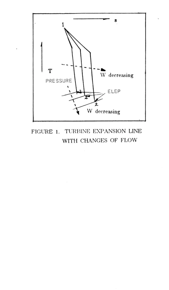
1 Turbine Expansion Line With Load Changes 67
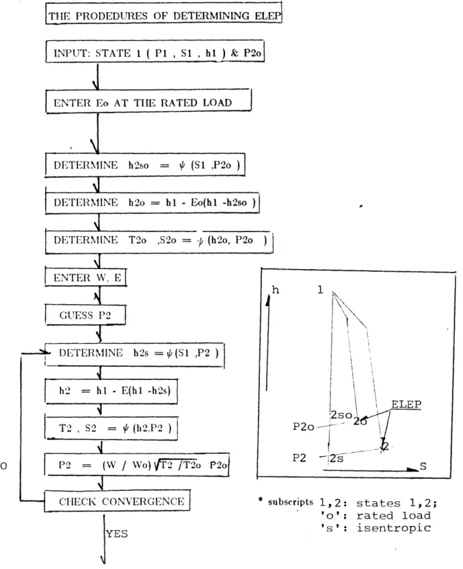
2 The Flowchart Describing The Determination Of The
Expansion Line End Points Of Turbines 72
3 Schematic Diagram Of The Selected System 79
4 Transient Response Of Pressure In The system With
The Ramp Input 85
5 Transient Response Of Temperature In The system With
The Ramp Input 85
6 Transient Response Of Pressure In The system With
The Ramp Input With Exaggerated Control Volume 86 7 Transient Response Of Pressure In The system With
CHAPTER 1
INTRODUCTION
The equation of state in the form of the Massieu Potential Function (MPF) has been derived in Part I. The resulting equation of
state was discussed in Section 4.2 of Part I, in terms of the criteria: accuracy, simplicity, .identification of saturation curve and physical meaning of the equation.
In this part, the equation of state is applied to two practical problems associated with steam turbine cycle calculations. The primary reason for the application was to evaluate, in the practical engineering situations, the equation of state according to the above-mentioned criteria. The secondary reason would be to examine the feasibility of obtaining a useful scheme of computation which may be immediately used. The two problems for the application of the equation of state are:
1) the determination of states on the expansion line including the expansion line end point(ELEP) of steam turbines at partial loads; and