Evidence from the American Mathematics Competitions
The MIT Faculty has made this article openly available.
Please share
how this access benefits you. Your story matters.
Citation
Ellison, Glenn, and Ashley Swanson. “Do Schools Matter for High
Math Achievement? Evidence from the American Mathematics
Competitions†.” American Economic Review 106, no. 6 (June 2016):
1244–1277.
As Published
http://dx.doi.org/10.1257/aer.20140308
Publisher
American Economic Association
Version
Final published version
Citable link
http://hdl.handle.net/1721.1/110279
Terms of Use
Article is made available in accordance with the publisher's
policy and may be subject to US copyright law. Please refer to the
publisher's site for terms of use.
1244
Do Schools Matter for High Math Achievement?
Evidence from the American Mathematics Competitions
†By Glenn Ellison and Ashley Swanson*
This paper uses data from the American Mathematics Competitions to examine the rates at which different high schools produce high-achieving math students. There are large differences in the frequency with which students from seemingly similar schools reach high achievement levels. The distribution of unexplained school effects includes a thick tail of schools that produce many more high-achieving students than is typical. Several additional analyses suggest that the differences are not primarily due to unobserved differences in student characteristics. The differences are persistent across time, suggesting
that differences in the effectiveness of educational programs are not primarily due to direct peer effects. (JEL H75, I21, I24, I28, R23)
High-achieving students make important contributions to scientific and technical fields, and educational productivity has been heralded as a vital source of com-parative advantage for the United States.1 It is therefore troubling that the United
States trails most OECD countries not only in average math performance, but also in the fraction of students who earn very high math scores.2 It is yet unclear how
1 Two notable examples of high-achieving high school students with a large economic impact are Microsoft’s Bill Gates, who coauthored a computer science paper as a Harvard freshman, and Google’s Sergey Brin, who finished in the top 55 on the 1992 Putnam Exam. See Hoxby (2003) for a discussion of education as a source of US comparative advantage in human-capital intensive industries; Krueger and Lindahl (2001) and Hanushek and Woessmann (2008) for surveys of the empirical literature on education and growth; and Altonji (1995), Levine and Zimmerman (1995), Rose and Betts (2004), Joensen and Nielsen (2009), and Altonji, Blom, and Meghir (2012) for evidence on math and the labor market.
2 Hanushek, Peterson, and Woessmann (2011) note that “most of the world’s industrialized nations” have a higher percentage of students reaching advanced levels on the 2006 PISA (Programme for International Student Assessment) test than does the United States. On the 2009 PISA math test, just 1.9 percent of US students achieved “Level 6” scores, whereas the OECD average was 3.1 percent and Singapore had 15.6 percent of its students at this level. PISA’s reading tests indicate that the United States is good at producing students with very high verbal achievement: the US’s percentage of “Level 6” reading students is well above the OECD average (1.5 percent versus 0.8 percent).
* Ellison: Department of Economics, MIT, 77 Massachusetts Avenue, Building E18, Room 269F, Cambridge, MA 02139, and NBER (e-mail: [email protected]); Swanson: The Wharton School, University of Pennsylvania, 3641 Locust Walk, CPC 302, Philadelphia, PA 19104, and NBER (e-mail: [email protected]). This project would not have been possible without Steve Dunbar and Marsha Conley at AMC, who provided access to the data as well as their insight. Hongkai Zhang and Sicong Shen provided outstanding research assistance. Victor Chernozhukov provided important ideas and help with the methodology. We thank several anonymous referees for their comments; we are particularly grateful to an anonymous referee who generously provided us with data that allowed us to extend our analysis. We also thank David Card and Jesse Rothstein for help with data matching. Financial support was provided by the Sloan Foundation and the Toulouse Network for Information Technology. Much of the work was carried out while the first author was a visiting researcher at Microsoft Research. The authors declare that they have no relevant or material financial interests that relate to the research described in this paper.
† Go to http://dx.doi.org/10.1257/aer.20140308 to visit the article page for additional materials and author disclosure statement(s).
best the United States might address this significant shortcoming. It seems obvious that high-quality schools would play an important role, but several recent papers that examine gifted programs and elite magnet schools have found further troubling evidence that these schools/programs do not appear to benefit marginal students.3
In this paper, we examine the questions of whether schools matter for high math achievement and whether there are many more students in the United States who would have reached high math achievement levels in a different environment. We examine the rates at which different schools produce high-scorers in the American Mathematics Competitions (AMC) contests and note that there are substantial dif-ferences across seemingly similar schools. We conduct several additional analyses to investigate whether these differences may be due to unobserved differences in underlying student ability. The analysis suggests that there are substantial differences in the effectiveness of schools’ educational programs and that the high-achieving students we observe are a small subset of those who would have reached high math achievement levels in a different environment.
Section I describes the primary data source for our study, the Mathematical Association of America’s AMC 12 contest. The contest is a 25-question multiple choice test on precalculus topics given annually to over 100,000 US students at about 3,000 high schools. The primary advantages of the AMC are that the test is explicitly designed to test depth of knowledge and high-level problem-solving skills and can distinguish among students at very high achievement levels. The pri-mary drawback, which will influence how we conduct the analysis, is that the test is taken by a nonrandom self-selected sample of students. We examine different levels of “high” achievement. Many of our analyses focus on counts of students within a school who score at least 100 on the 2007 AMC 12. One can think of this as roughly comparable in difficulty to scoring 800 on the math SAT, but measured using a more reliable test that emphasizes greater depth of knowledge.4 We also
examine students at a substantially higher achievement level: those scoring at least 120 on the AMC 12, which puts them well above the 99.9th percentile in the US population.5 We match AMC schools to data from the census, National Center for
Education Statistics (NCES), college board, and ACT to obtain demographic data and other covariates and conduct most of our analyses on the subsample of pub-lic, coed, nonmagnet, noncharter US high schools that administer the AMC 12 and could be matched to the other databases. Section II discusses the data in more detail.
Section III begins with our most basic observation: some schools produce many more AMC high-scorers than do other schools with similar demographics. Negative binomial regressions show that there are a number of strong demographic predic-tors of high achievement. For example, a 1 percentage point increase in the fraction of adults with graduate degrees is associated with a seven percent increase in the number of AMC high-scorers, and a one percentage point increase in the fraction of the population that is Asian American is associated with a two percent increase. 3 See Abdulkadiro˘glu, Angrist, and Pathak (2014); Bui, Craig, and Imberman (2014); and Dobbie and Fryer (2014).
4 The highest possible score on the math SAT is 800 and is achieved by approximately one percent of SAT test-takers.
5 One noteworthy student who reached this level five years earlier is Facebook’s Mark Zuckerberg, whose name appears on the AMC’s 2002 distinguished honor roll for having scored 121.5.
But the most important finding is that the demographic effects are far from sufficient to account for the observed differences in the rates at which different schools are producing high-achieving students. The excess variance parameter in the negative binomial model can be thought of as an estimate of the magnitude of the unobserved multiplicative “school effects” that would be necessary to account for the observed dispersion. We find that the necessary variance is 0.73 at the 100-AMC level and 2.18 at the 120-AMC level: e.g., it is as if a school that is one standard deviation above average produces students who score at least 100 on the AMC 12 at a rate that is 85 percent ( ≈ √_0.73 ) greater than average.
Section IV examines the distribution of the unobserved “school effects.” The motivation for examining these distributions, rather than being satisfied with know-ing the variance, is similar to that for the literature on the heterogeneity in teacher value-added: it is useful to know, for example, if the variance seems to be due to the existence of a subset of low-performing schools in which students are very unlikely to become AMC high-scorers, or if it is due to a small (or big) set of schools that produce high-scorers at much (or slightly) higher than average rate.6 Counts
of high-achieving students are inherently small, so one cannot precisely estimate a school fixed effect for any one school. But one can estimate the distribution of school effects across schools.7 Formally, we implement a nonparametric estimator
for the distribution of the unobserved component in a model in which schools pro-duce high-scorers at Poisson rates which differ due to observed school and local area characteristics and an unobserved component.8 We estimate that many schools
are producing high-scorers at a well below average rate, e.g., 32 percent of schools appear to be producing high-scorers at less than one-half of the average rate. And a striking finding is that there appears to be thick upper tail of schools that produce AMC high-scorers at many times the average rate. For example, we estimate that more than 11 percent of schools are producing AMC high-scorers at more than twice the rate one would expect given their demographics and 1 percent of schools are producing AMC high-scorers at more than five times the average rate.
The “school effects” we estimate can be thought of as indexes that conflate mul-tiple factors that lead to heterogeneity in outcomes. They will reflect differences in causal effects across school environments. But they will also reflect other less inter-esting sources of outcome heterogeneity: differences due to potentially observable demographic differences not captured by variables in our dataset; unobservable dif-ferences in student ability due to location decisions of parents of gifted children; and even less interestingly, differences in the fraction of the high-achieving math stu-dents at each school who take the AMC 12 test. Section V presents several additional analyses aimed at assessing whether effects of the less interesting types are likely to account for a substantial portion of the heterogeneity we have found. To examine 6 See, for example, Gordon, Kane, and Staiger (2006) for plots of the estimated distribution of teacher qualities obtained by shrinking estimated teacher fixed effects to take out purely random variation.
7 Although we have AMC data at the individual level, we only observe some coarse demographic variables and hence have chosen to estimate school effects rather than, for example, multilevel models as in Skrondal and Rabe-Hesketh (2009).
8 The method involves a series expansion similar to that of Gurmu, Rilstone, and Stern (1999) but relying on a different characterization of the likelihoods designed to be more appropriate for potentially fat-tailed distributions. Appendix I contains more detail on the estimation along with Monte Carlo estimates illustrating the performance of the estimator.
the effects of heterogeneity in participation rates, we compare the magnitudes at the AMC 100 and AMC 120 levels. (We argue that selection into test-taking is not important at the higher level.) We explore the importance of unobserved heteroge-neity in student populations in two ways: we examine counts of students achieving perfect scores on the math sections of the SAT and ACT which should be similarly affected by demographic differences but less sensitive to differences in the depth of knowledge developed by the school environment; and we compare school effects estimated from counts of all high-scoring students with school effects estimated from counts of high-scoring girls. A motivation here is that unobserved demo-graphic differences that impact location decisions should not differ much between high-ability male and female students, whereas differences in school environments, such as whether a school’s high-level math programs are female-friendly, would lead to gender-related differences.9 Taken together, these analyses provide evidence
that unobserved heterogeneity in performance across schools is much greater than can be explained by student heterogeneity or selection into taking the test.
Section VI presents several analyses intended to provide insight into the mech-anisms that may be making some schools more effective than others. We begin by exploring one very simple mechanism: there could be large effects on the number of students with upper-tail scores if some schools increase their students’ scores by a constant and the distribution of scores has a thin-tailed distribution. We look for such a mechanism by including school-average SAT/ACT scores as a covari-ate. We find little effect, suggesting that our school effects reflect something salient for high-achieving students in particular. Although we have discussed our school effects as indexes reflecting heterogeneity in outcomes, it is more accurate to think of them as measures of the strength of the forces needed to produce the observed degree of clustering of high-scoring students. Such clustering could be generated by unobserved heterogeneity in school quality, but it could also be an artifact of strong peer effects among high-scoring students. Using a formal model similar in spirit to that of Ellison and Glaeser (1997), we note that, with a single observation on each school, one cannot distinguish unobserved heterogeneity in school quality from peer effects as a source of such clustering. However, one can estimate the relative impor-tance of school quality versus peer effects with multiple observations per school if school quality is persistent and peer effects are not felt across periods. We present such an estimate derived from comparing the agglomeration of 2007 high-scorers to the coagglomeration of 2007 and 2003 high-scorers. It suggests that differences in school environments are not primarily due to within-cohort peer effects. Finally, we present some qualitative observations on some of the most unexpectedly suc-cessful schools. Among our observations are that a number of these schools have a long-serving “star” teacher.
Our work is related to a number of literatures. One is the literature on the effective-ness of elite schools and gifted programs. Recent papers by Abdulkadiro˘glu, Angrist, and Pathak (2014); Dobbie and Fryer (2014); and Bui, Craig, and Imberman (2014) examine the effects of elite magnet schools and gifted programs on high-ability students using regression discontinuity designs. Their common finding that the 9 Ellison and Swanson (2010) document that, at the highest performance levels, female high-scorers are drawn from a much smaller set of super-elite schools than are male high-scorers.
programs have no impact on the test scores of marginal admitted students is striking given that one might have expected the students to benefit from superior peers even absent superior instruction and has attracted a great deal of attention. Our contrast-ing suggestion that schools are important for gifted students could potentially be reconciled in various ways: the tests we study assess more in-depth understanding and problem-solving skills; effects of programs on marginal admitted students could be very different from the effects on students in the opposite tail; or it could be that the particular gifted programs studied in the previous papers are not very effective but the programs of many other schools in our sample are.10
A second related literature on gifted students is that on low-income students with high SAT/ACT scores missing from the student bodies of elite colleges. Several authors have noted that there are many such students and a proximate cause is that many low-income high school students with high SAT/ACT scores do not apply to elite colleges.11 Hoxby and Avery (2013) provide the most comprehensive analysis
and document that such students are disproportionately found in areas where they are unlikely to have the opportunity to attend a selective high school, to study with teachers who attended selective colleges, and to interact with many high-achieving peers. Our findings are somewhat analogous in that we are suggesting that there are many students who could have achieved an educational distinction in a dif-ferent environment. One difference, however, is that (by focusing on schools that offer the AMC) we are focusing on missing students from within a set of relatively high-achieving high schools. Presumably, the set of students identified in the papers noted above would be a substantial additional source of students who could have been high math achievers.12
There is a much larger literature on quality differences across schools affect-ing average achievement. This includes many papers examinaffect-ing how inputs affect achievement and papers that focus on differences in productivity related to compe-tition, vouchers, charter schools, etc.13 Many of these papers control for selection
effects and estimate causal effects relevant to school reform debates. The smaller literature examining residual variance is more closely related.14 These papers
gen-erally find that unobserved school-level heterogeneity is much less important than are student and neighborhood characteristics for predicting test scores, graduation rates, and labor market outcomes. Our findings that schools appear to matter a great deal to high-achieving students may sound conflicting, but could be reconciled in several ways: it has been noted previously that differences that are small relative to within-school variation and/or demographic differences can still be large in abso-lute terms; environmental differences that produce small differences in mean scores
10 Angrist and Rokkanen (2015) examine additional test scores of admitted students and argue that Boston Latin School also appears to have little impact on the performance of students farther from the cutoff on state proficiency tests.
11 See Bowen, Kurzweil, and Tobin (2005); Avery et al. (2006); and Pallais and Turner (2006).
12 Two other relevant literatures on high-achieving students are the literature on cross-sectional differences in high achievement (e.g., Hanushek, Peterson, and Woessman 2011; Pope and Sydnor 2010; and Andreescu et al. 2008), and the literature on how proficiency-focused reforms may harm high-achieving students (e.g., Krieg 2008; Neal and Schanzenbach 2010; and Dee and Jacob 2011.)
13 See Coleman (1966); Hanushek (1986); Card and Krueger (1992); Hoxby (2000, 2003); Angrist et al. (2002); Hoxby, Murarka, and Kang (2009); Abdulkadiro˘glu et al. (2011); and Dobbie and Fryer (2011).
14 See Jencks and Brown (1975); Solon, Page, and Duncan (2000); Rothstein (2005); and Altonji and Mansfield (2010).
could have a magnified impact when one looks at tail outcomes; or there could be more true heterogeneity in school quality relevant to high math achievement.
Our methodology is related to the literature on measuring agglomeration, includ-ing papers such as Ellison and Glaeser (1997); Marcon and Puech (2003); Duranton and Overman (2005); Bayer and Timmins (2007); and Ellison, Glaeser, and Kerr (2010). Whereas many indexes are motivated as a scalar representation of the strength of agglomerative forces, we quantify agglomerative forces by estimating a distribution of effect sizes. Our discussion of peer effects and unobserved hetero-geneity is also related to Graham (2008), which derives general conditions under which peer effects and unobserved heterogeneity can be separately identified by looking at residual covariances and includes an application to peer effects in the STAR experiment.
I. The American Mathematics Competitions
The American Mathematics Competitions is the largest and most prestigious series of math competitions for US high school students. The AMC 12 contest is a 25-question multiple choice test administered in over 3,000 US high schools. About 100,000 students participated in 2007.15 Our primary motivation for examining
AMC data is that we feel that the AMC 12 is superior to any other test administered at comparable scale in its reliability and validity for identifying students at very high levels of math achievement.
Regarding reliability, the most natural comparison is to the math portion of the SAT reasoning test. We regard the SAT as not reliable above the ninety-seventh per-centile: when students who score an 800 (a perfect score which is the ninety-ninth percentile) retake the math SAT, only 15 percent score 800 again and their average retake score of 752 is a ninety-seventh percentile score. Scoring 100 on the AMC 12 can be thought of as roughly comparable in difficulty to scoring 800 on the SAT. Scoring 120 on the AMC 12 can be thought of as at least an order of magnitude more difficult and places students above the 99.9th percentile of the SAT population. In a striking contrast to the SAT, the AMC 12 remains well calibrated even at the higher of these levels.16
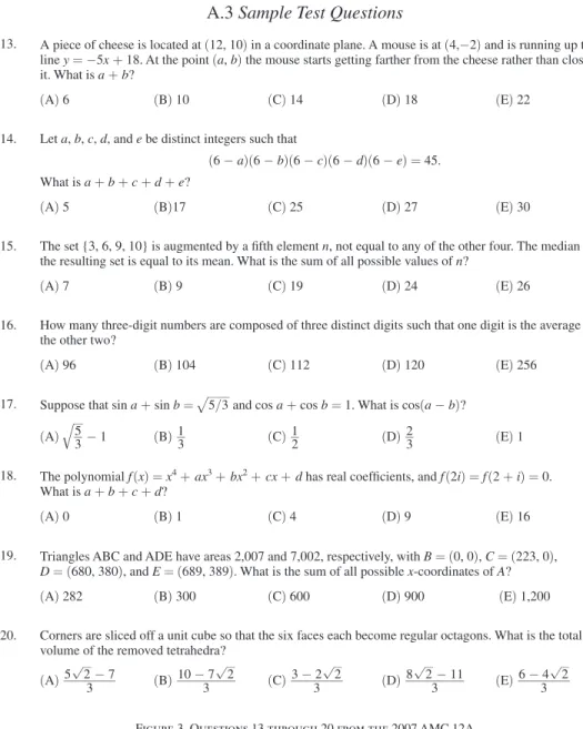
Regarding validity, we would argue first that a casual inspection of the tests strongly suggests that the AMC 12 is superior to the SAT as a test of important math skills. A student is awarded an 800 score on the math SAT only if he or she can work through 54 relatively straightforward problems in 70 minutes without making a single mistake. The AMC 12 consists of 25 problems on a wide range of precalcu-lus topics. They generally require greater depth of knowledge and problem solving skills than SAT questions. To score 100 on the AMC 12, a student need only solve 14 of the 25 problems in 75 minutes. To give a sense of what this entails, Figure 3 in the 15 The AMC 12 is the first stage of a series. In 2007, about 8,000 AMC 12 high-scorers were invited to take the American Invitational Mathematics Examination (AIME). About 500 AMC/AIME high-scorers were then invited to take the USAMO. Finally, about 50 high-scorers from the USAMO were invited to a summer training program, from which 6 students were chosen to form the US team for the International Mathematical Olympiad.
16 The AMC 12 is offered on two different dates each year. As noted in Ellison and Swanson (2010), students who scored 95 to 105 on the first 2007 date and retook the test averaged 103 with a standard deviation of 11 on the retake. Students who scored 115 to 125 on the first date averaged 119 with a standard deviation of 10 on the retake.
Appendix contains questions 13 through 20 from the 2007 AMC 12. Questions are arranged in increasing difficulty, so students will probably need to solve at least two or three of these problems to score 100. Scoring 120 on the AMC 12 is much harder. It requires answering at least 19 questions correctly. Hence, it requires that students be able to work much more quickly and solve essentially all of the questions shown in the figure.
Statistical evidence of validity can also be provided by examining how high AMC scorers do when taking other tests. To develop evidence on how well AMC scores predict success on SAT-style tests, we obtained AMC and SAT scores for 195 quasi-randomly selected MIT applicants. Table 1 reports the mean score and the fraction of 800s that students obtained when they first took the math SAT as a function of their 2007 (eleventh grade) AMC 12 score.17 The table provides striking
evidence that the AMC 12 is much more powerful predictor of students’ ability to achieve a high SAT score than is the SAT itself. To develop evidence on how well AMC scores predict success in a very different important environment—solving more difficult open-ended problems—we gathered data from two states, Georgia and Massachusetts, which have state-level competition series that start with a broadly administered multiple choice test and culminate with tests that ask students to solve more open-ended problems and write some formal proofs.18 Georgia’s
2007 contest started with 1,440 students from 88 schools. At the end, 3 students were named as winners and 27 were awarded honorable mention. Despite these very long odds and the proof orientation of the final test, 15 of the 20 students at participating schools who had scored at least 120 on the 2007 AMC 12 made the top 30.19 The 2007 Massachusetts contest started with 2,000+ students from roughly
60 schools and 20 students were named as winners. Students scoring at least 120 on the 2007 AMC 12 could not possibly have succeeded at a comparable rate on the Massachusetts contest; there were 47 such students at participating schools. But the slightly more select sample of 22 students who had scored at least 129 on the AMC 12 were again remarkably successful given the long odds and very strong field: 12 of the 22 finished in the top 20. We conclude that the AMC 12 does remarkably well in identifying students with high-level math skills.
The primary drawbacks of the AMC 12 as a research tool are that it is only admin-istered in a nonrandom subset of US high schools and that students self-select into participation. The 3,000 AMC-offering schools are only about 10 percent of the total number of US high schools. The fraction of high-achieving US high school students who can take the AMC 12 in their high school is much higher than 10 per-cent—schools’ decisions to offer the AMC 12 are highly correlated with student demographics—but still probably only about 50 percent.20 The lack of
univer-sal administration makes it impossible for us to provide estimates of the number of high-achieving math students nationwide. However, we can work around this 17 The final column contains data from the College Board on how students with an 800 SAT perform when they retake it.
18 See Figure 4 in the Appendix for two sample problems from Georgia’s 2007 contest. 19 Each of the three winners scored at least 132 on the AMC 12.
20 One statistic we can provide to support this is that 58 percent of the students who were named Presidential Scholar candidates (an honor based on having high combined math plus reading SAT or ACT scores) attended a high school that offered the AMC 12.
drawback by focusing our analyses on heterogeneity in achievement within the set nonmagnet, noncharter, coeducational public schools that administer the AMC 12.
The second drawback of the AMC is more problematic: some schools may be more aggressive than others in encouraging their best math students to take the AMC 12. This will be a source of apparent performance differences even when edu-cational environments are identical. The main thing we will do to try to get a sense for how this may be affecting our results is to perform some analyses both on the set of students scoring 100 on the AMC 12 and on the set of students scoring 120 on the AMC 12.
II. Data
The 2007 AMC 12 contest consisted of two separate tests administered on dif-ferent dates: schools could give the 12A exam on February 6, 2007 and/or the 12B exam on February 21, 2007.21 Our raw data are at the individual level and contain
the test date (A or B), score, student ID, school ID, grade, gender, and home zip code. For most of our analyses we work with school-level aggregates. We merge the AMC data with several other databases. First, we match the schools to the schools in the NCES Common Core of Data (CCD) and Private School Survey (PSS) by school name, city, and state.22 Second, we obtain additional demographic
vari-ables by matching the schools to census data on the zip code in which the school is located.23 Finally, we matched the schools to a database containing counts of SAT/
ACT takers, average SAT/ACT scores, and counts of students with perfect scores by school.24
21 The primary motivation for having two test dates is to facilitate the participation of schools that may be on vacation or have some other conflict with one date. About 64 percent of US schools administer only the 12A exam, with 28 percent administering only the 12B, and 8 percent administering both.
22 The AMC school IDs are usually a school’s CEEB (College Entrance Examination Board) code. We obtain the school name, city, and state using the CEEB search program on the College Board’s website. Of the 3,730 schools with numerical CEEB codes in the AMC data, 3,105 were matched to schools in the NCES data. Three hundred eleven of the unmatched 625 schools do not appear in the NCES data because they are not in the United States. A further 160 could not be matched because the AMC school IDs were not valid CEEB codes. The remaining 154 unmatched schools will include among others, private schools that do not appear in the NCES survey data because private schools are not required to fill out the PSS. Among the matched schools, a further three were dropped because they were missing covariates used in the estimations described below.
23 Such data were available for 3,021 of 3,105 AMC schools.
24 We drop schools from the sample if we are unable to match to the SAT data. We also drop if the ACT data are missing and the school is located in a state where more than 20 percent of students take the ACT, or if the SAT data are missing and the school is located in a state where more than 20 percent of students take the SAT. We drop all data from Arkansas, Illinois, and Wyoming, where all ACT data are missing. A total of 157 schools are dropped for one of these reasons.
Table 1—SAT Math Scores for a Sample of Students with AMC 12 Scores in Various Ranges AMC 12 scores
Prior 800 SAT
80s 90s 100s 110s 120s 130s 140s
Mean on first math SAT 711 745 773 774 791 793 800 752
Percent with 800 on first SAT 0 19 35 38 65 60 100 15
Our primary variables of interest will be counts of students in each school scoring at least 100 or 120 on the AMC 12.25 In defining these variables we use the count of
students scoring at least the cutoff on the 12A contest if the school administered the 12A and the count scoring at least the cutoff on the 12B exam if the school offered only the 12B.26 In our analyses using SAT/ACT data we use both school-average
scores and the number of students with perfect scores. In defining these variables, we use a student’s SAT score if the student took the SAT and the ACT score if the student did not.27
Most of our analyses will be run on the set of public, coed, nonmagnet, nonchar-ter schools that adminisnonchar-tered the AMC 12. Eliminating magnet schools is import-ant to make it feasible to control for the quality of the student population using available demographic data on the school and its zip code. In addition to drop-ping 800 schools listed by the NCES as being private, noncoed, magnet, or charter schools, and 3 schools missing NCES data on school demographics, we dropped an additional 76 schools after a manual examination: we examined all schools that were among the 200 largest positive outliers in preliminary regressions of the count of AMC and SAT high-scorers on demographic variables, as well as schools outside the first to ninety-ninth percentile range in percent of female students, and dropped schools that offered a special program that seemed likely to attract high-achieving math/science students from outside a neighborhood attendance area.
Note that in aggressively dropping schools with magnet-like features, we are omitting many schools with programs explicitly designed to promote high math achievement. Hence, while our inability to eliminate all self-selection is a factor that will lead us to overstate the prevalence of high-achieving schools, our data construction also has a potentially strong bias working in the opposite direction. For example, we drop Rockdale County HS in Conyers, GA from our dataset because it houses a school-within-a-school, the Rockdale Magnet School for Science and Technology, which enrolled about 40 students per grade in 2007. However, even if one were to think of these students as the 40 best in the entirety of Rockdale County, the school’s performance would be impressive. The entire county’s popu-lation is only about 85,000 and given its demographics (e.g., majority free/reduced lunch, 60 percent African American, 2 percent Asian American), the three AMC 12 high-scorers from the school in 2007 are about ten times as many as one would have expected to find in the entire county. And the fact that the school has special
25 The AMC 12A and 12B are not necessarily identical in difficulty. To control for this, we adjust the AMC 12B cutoffs such that, within the sample of 2,286 students who took both exams, the count of students scoring above 100 on the 12A is equivalent to the count of students scoring above the adjusted cutoff on the 12B. We perform a similar adjustment for the 120 cutoff. Based on this adjustment, we use 12B cutoffs of 108 and 123 as equivalent to 100 and 120 on the 12A.
26 Note that we do not count students from a school that offered both the 12A and the 12B if they did not partic-ipate in the 12A and then scored above the cutoff on the 12B. We count in this way to be conservative in measuring heterogeneity: schools that administer the AMC 12 on both dates are disproportionately high-achieving schools and we want to eliminate any advantage they may obtain from increasing participation by offering both test dates.
27 We convert ACT scores to SAT equivalents using SAT/ACT concordance data from Lavergne and Walker (2001), which relied on 1999–2000 data, and Dorans (1999), which relied on 1994–1996 data. Each source specifies a range of SAT scores corresponding to each ACT score. We construct an implied SAT equivalent for each source using their tables directly, and take the average of the implied scores across sources to generate our SAT/ACT correspondence. Results are not sensitive to the methodology. One additional school is dropped because the school-average ACT score in the SAT/ACT database is equal to four.
programs makes it all the more plausible that features of the school environment are responsible for this success.
Table 2 contains summary statistics for the merged database of 1,984 sam-ple schools offering the AMC. The average school has 0.8 students score at least 100 on the AMC 12 and 0.11 students score at least 120.28 The number of female
high-scorers is substantially lower. Relative to the average public, noncharter, nonmagnet, coed high school in the United States, the average school offering the AMC is larger, has more Asian American and fewer black and Hispanic students, is less likely to receive Title I funding, and has fewer students qualifying for the free lunch program. Sample AMC schools are also located in wealthier, more urban zip codes with more highly educated adults. As expected given school and region demographics, AMC schools also perform better than the average US public school on the SAT math, having higher mean scores and more students with perfect scores.
III. Differences in High Math Achievement across Schools
In this section, we bring out two basic facts. There are large systematic differ-ences in the rates at which different schools produce high math achievers related to the schools’ demographics. And there are also large differences among seemingly similar schools.
A. Achievement Gaps
In this section we explore the magnitude of various achievement gaps among high-achieving math students by examining the relationship between the number 28 In the full set of 3,105 schools that we matched to the NCES data, the mean number of students scoring at least 100 on the AMC 12 is 0.93, reflecting that the dropped schools (which are mostly private, magnet, or magnet-like) have more high-scorers per school.
Table 2—School-Level Summary Statistics
Variable Mean SD
Count AMC > 100 0.80 1.87
Count AMC > 120 0.11 0.49
Count AMC > 100 female 0.12 0.45
Count AMC > 120 female 0.01 0.11
Number of students 1,452.02 819.90
School fraction Asian 0.07 0.12
School fraction Black 0.09 0.14
School fraction Hispanic 0.09 0.13
School fraction female 0.49 0.02
Title I school 0.21 0.41
School fraction free lunch 0.15 0.14
log(zip median income) 10.84 0.38
Adult fraction BA 0.20 0.09
Adult fraction grad 0.13 0.09
Zip fraction urban 0.78 0.32
Count perfect SAT/ACT 1.67 3.59
Average SAT/ACT 526.73 41.79
of high AMC scorers in a school and its demographics. The first column of Table 3 presents coefficient estimates (with standard errors in parentheses) from a negative binomial regression with the number of students in a school scoring at least 100 on the AMC 12 as the dependent variable. The estimates indicate that several observ-able characteristics of a school/neighborhood are strong predictors of the number of high math achievers that a school will produce. Parental education is very important: a one percentage point increase in the fraction of adults with bachelor’s and graduate degrees increases the expected number of AMC high-scorers by 2.5 and 7.0 percent, respectively. Racial and ethnic composition also matters. The estimates suggest that a one percentage point increase in the Asian American population increases the expected number of AMC high-scorers by 1.8 percent. We also find that there are fewer high AMC scorers in schools that have more Hispanic students and those that have more low-income students qualifying for the free lunch program.
One demographic variable that would be significant in most regressions of school-mean standardized test scores on demographics that does not have the expected effect here is that the number of AMC high-scorers is not higher in higher-income areas. Several potential explanations for the lack of an income effect are possible: e.g., it could reflect nonlinearity in the income-AMC relationship ( AMC-participating schools are disproportionately located in upper-income areas) or it could be due to a selection effect with participating schools in low-income areas being highly nonrepresentative.29
B. Magnitudes of Differences among Seemingly Similar Schools
In this section, we document that there are also large differences among seem-ingly similar schools. One way to do this is via the negative binomial regression estimates. One justification for the negative binomial model is if the number of high-scorers in school i is Poisson with mean e X i β u
i , with u i being a multiplicative gamma-distributed unobserved shock to a school’s production rate that has mean 1 and variance α .30 For example, a school would have a u
i of 0.5 if each of its students were only one-half as likely to score 100 on the AMC 12 as were students at the average school with comparable demographics, and a u i of 1.5 if its students were 50 percent more likely to succeed than would be expected given the demographics. In our negative binomial regression of the number of students scoring at least 100 on the AMC 12 on school demographics, the estimated variance of the multiplicative random shock is α ̂ = 0.73 . A variance of 0.73 corresponds to a standard deviation of 0.85, i.e., a school that is one standard deviation above average is producing AMC high-scorers at 185 percent of the average rate and a school that is one standard devi-ation below average is producing AMC high-scorers at just 15 percent of the average rate. For the variance to be this large there must be a substantial number of schools
29 The income effect becomes smaller in magnitude but remains negative and significant if we drop the Title 1 and free lunch variables.
30 This model is sometimes referred to as the Negbin 2 model. See, e.g., Cameron and Trivedi (1986) and Greene (2008) for a discussion of negative binomial functional forms.
producing AMC high-scorers at a small fraction of the average rate and/or a number of schools producing AMC high-scorers at two or more times the average rate.31
31 The estimate is highly significant and a likelihood ratio test rejects the Poisson alternative at an extremely high significance level.
Table 3—Demographic Predictors of High Math Achievement Count of high-scorers in school
Perfect Female
Variable AMC12 ≥ 100 AMC12 ≥ 120 SAT/ACT AMC12 ≥ 100
log(number of students) 1.14 1.13 1.47 1.23 1.22 1.38
(0.10) (0.12) (0.28) (0.07) (0.17) (0.22)
Adult fraction BA 2.50 2.10 6.74 1.34 1.27 3.14
(0.73) (0.78) (1.81) (0.49) (0.49) (1.44)
Adult fraction grad 7.04 7.32 7.75 5.33 5.29 7.01
(0.54) (0.67) (1.18) (0.35) (0.74) (0.94)
School fraction Asian 1.81 1.80 2.17 2.35 2.36 1.74
(0.28) (0.30) (0.62) (0.16) (0.34) (0.48)
School fraction Black −0.77 −0.60 −1.44 −1.18 −1.26 −1.19
(0.43) (0.44) (1.34) (0.32) (0.36) (1.00)
School fraction Hispanic −1.77 −1.77 −3.26 −0.83 −0.86 −1.55
(0.45) (0.48) (1.43) (0.31) (0.31) (0.98)
log(zip median income) −0.70 −0.67 −1.40 −0.18 −0.14 −0.72
(0.15) (0.16) (0.35) (0.10) (0.10) (0.28)
School free lunch fraction −2.26 −2.47 −3.72 −2.56 −2.39 −2.70
(0.59) (0.64) (1.80) (0.44) (0.53) (1.30)
Title 1 school −0.04 −0.04 −0.23 0.02 0.01 0.03
(0.11) (0.11) (0.29) (0.07) (0.07) (0.22)
Zip fraction urban 0.20 0.20 0.60 0.46 0.49 0.14
(0.24) (0.25) (0.78) (0.18) (0.18) (0.55)
School fraction female −0.30 −0.36 1.86 2.57 2.53 2.77
(2.24) (2.26) (5.94) (1.53) (1.56) (4.69)
log(SAT/ACT participation) 0.95 0.95
(0.10) (0.15)
Constant −2.35 −2.65 −1.73 −7.66 −7.98 −7.48
(2.00) (2.10) (4.87) (1.44) (1.68) (4.01)
log-likelihood −1,899.1 −1,893.6 −493.4 −2,372.5 −2,371.5 −605.6
Pseudo R 2 0.19 0.21 0.27 0.19
Estimation method NB semi-P NB NB semi-P NB
Estimated var( u i ) 0.73 0.96 2.18 0.23 0.23 0.95
(standard error) (0.08) (0.17) (0.50) (0.03) (0.09) (0.29)
Observations 1,984 1,984 1,984 1,984 1,984 1,984
High scorers 1,596 1,596 211 3,307 3,307 243
Notes: Results of negative binomial regression and semiparametric model estimation. Outcomes are counts of high achievers (students scoring more than 100 or 120 on the AMC 12 or with 800 (36) on the SAT (ACT) math) in each school.
Sources: School demographics are from the NCES Common Core of Data for 2005–2006; zip code demographics are from the 2000 US census. The school sample includes coed, noncharter, nonmagnet public schools that offered the 2007 AMC 12.
We conclude that demographic differences account for a substantial portion of the variation across schools in the number of students who achieve high AMC scores, but that there are also substantial differences across seemingly similar schools.
IV. Distributions of “School Effects”
We noted above that the negative binomial model can be regarded as providing an estimate of the variance of the unobserved school effects that we would need in addition to the demographic differences to reproduce the observed heterogeneity in the counts of AMC high-scorers. Excess variance, however, can take many forms: it may be due to a set of underachieving schools that produce very few high-scorers, or to a small (or large) set of extreme (or not so extreme) overachieving schools, etc. In this section, we provide estimates of the distribution of school effects that would lead to the distribution of outcomes observed in the data. One observation is that the distribution includes a thick tail of schools that produce many more AMC high-scorers than one would expect given their demographics.
Suppose the number of AMC high-scorers in school i , y i , is distributed Poisson
(
λ i)
, where λ i = e X i β u i , X i is a vector of observable characteristics, and u i is an unobserved “school effect” with a multiplicative effect on the Poisson rate. We assume that the school effect u i has an unknown density f . Appendix A1 describes a methodology for estimating both the coefficients β on the observable characteristics and the distribution f of the unobserved school effects. In a nutshell, we estimate the density via a series estimator: we model f (x) as a product of a gamma-like term, x α e −x , similar to that used in the negative binomial model and an orthogo-nal polynomial expansion, note that different coefficients on the polynomial terms produce different likelihoods of seeing 0, 1, 2, etc. high-scorers, and use maximum likelihood estimation to find a density that comes closest to matching the observed frequencies of the outcomes conditional on the demographics.We estimate the model on the same dataset as the negative binomial regression of the previous section: we use the count of students scoring at least 100 on the AMC 12 as the dependent variable and include the same set of demographic controls. The second column of Table 3 reports the estimated coefficients on the demographic controls. They are similar to the negative binomial estimates in the first column, indicating that those estimates are robust to the more flexible modeling of the unob-served heterogeneity. Indeed, a comparison of the maximized log-likelihoods at the bottom of the table shows that the semiparametric model fits the data only slightly better than the negative binomial model discussed in the previous section, suggest-ing that the true distribution of the u i is fairly similar to a gamma distribution.32
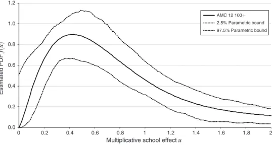
Our primary interest here is in the distribution of the school effects. We note first in Table 3 that relaxing the assumption that the u i are gamma-distributed increases the estimated variance from 0.73 to 0.96. Panel A of Figure 1 graphs the probability density function from which the unobserved school effects u i are estimated to be 32 See Table 5 in the online Appendix for a comparison of predicted counts under the Poisson, negative bino-mial, and semiparametric models to the actual counts in the data. The table includes, for each model, a χ 2 test of goodness-of-fit; the tests confirm our visual assessment that the actual data reject the Poisson model at a high level of significance, but they do not reject the negative binomial or semi-parametric models at conventional levels, hav-ing p-values of 0.7 in each case.
drawn. The x -axis corresponds to different possible values of the unobserved effect: e.g., a value of u = 1 corresponds to a school that produces AMC 12 high-scorers at exactly the mean rate given its demographics, a value of u = 0.5 corresponds to a school that produces high-scorers at half of this rate, etc. Informally, the curve is like a histogram giving the relative frequency of the values of u in the population of schools. Substantial differences between schools with similar demo-graphics are evident: the distribution is not tightly concentrated around u = 1 . Instead, there are a large number of schools that produce AMC 12 high-scorers at well below the average rate: e.g., about 32 percent are estimated to produce
0.0 0.2 0.4 0.6 0.8 1.0 1.2 0 0.2 0.4 0.6 0.8 1 1.2 1.4 1.6 1.8 2 Estimated PDF f( u)
Multiplicative school effectu Panel A. Distribution of school effects: students scoring 100+ on the AMC 12
0.90 0.91 0.92 0.93 0.94 0.95 0.96 0.97 0.98 0.99 1.00 2 3 4 5 6 7 8 Estimated CDF F( u)
Multiplicative school effect u Panel B. Detail on CDF in the upper tail
AMC 12 100+ 2.5% Parametric bound 97.5% Parametric bound AMC 12 100+ 2.5% Parametric bound 97.5% Parametric bound
high-scorers at less than half of the average rate. At the other end, there are many highly successful schools producing high-scoring students at 50 to 100 percent above the average rate. The dashed lines in the figure are 95 percent confidence bands for the estimated density.33 They indicate that the estimates are fairly precise
throughout most of the range.
A striking feature of the distribution that is not immediately apparent from the probability density function (PDF) graph is that the estimates indicate that there is a thick upper tail of extremely successful schools. Panel B of Figure 1 illustrates this better by graphing in bold the cumulative distribution function (CDF) of the esti-mated distribution for u ranging from 2 to 8. The estimates indicate that 11 percent of schools are estimated to be producing high-scorers at more than twice the average rate and there is a substantial mass (about 1 percent) producing high-achieving stu-dents at more than five times the average rate for a school with their demographics. The dashed lines again give a 95 percent confidence interval. They indicate that the thick tail is a statistically significant phenomenon.
V. Challenges to the Interpretation of the School Effects
As we noted earlier, the “school effects” we have estimated conflate multiple factors. They will reflect differences in causal effects of school environments on potential high math achievers. But they will also reflect other less interesting sources of outcome heterogeneity: demographic differences not captured by variables in our dataset; differences in unobserved student ability attributable to location decisions made by parents of gifted children; and even less interestingly, differences in the fraction of the high-achieving math students at each school who take the AMC 12 test. In this section, we present several auxiliary estimates aimed at providing some insights on the importance of these less interesting sources of outcome heterogene-ity. We will argue that they do not seem sufficient to account for the variation we have found.
A. Selection into Test-Taking: Evidence from Extreme High Achievers
A portion of the “school effects” we have reported will be due to differences in the AMC 12 participation rates for high-achieving math students from different schools. The primary way in which we can provide some evidence of whether this could be driving our results is to provide additional estimates derived from counts of students at even higher achievement levels.
Students scoring at least 120 on the AMC 12 can be thought of as well above the 99.9th percentile among college-bound students. The unique ability of the AMC 12 to distinguish among such extreme high achievers makes it possible to examine their agglomeration as well. We think that there are many students at AMC-offering schools who would have scored 100 if they had taken the AMC 12, but who did not take the test. We believe, however, that the fraction of students at AMC-offering 33 The confidence bands in this figure were generated using the parametric bootstrap procedure as described in the online Appendix. We also generated confidence bands using the nonparametric bootstrap procedure described there. They are quite similar (though slightly wider).
schools who would have scored 120 if they took the AMC 12, yet chose not to participate, is much smaller. Hence, we can compare results obtained with an AMC 12 cutoff of 100 to results obtained with an AMC 12 cutoff of 100 to see if results change when selection into test-taking becomes less important. Moreover, we believe that the issue of selection into test-taking is small in absolute terms at the 120 level and hence results with the 120 threshold cannot be greatly affected by selection into test-taking. We believe this for a few reasons. First, scoring 120 on the AMC 12 requires both a great deal of natural ability and a lot of effort dedicated to learning high school mathematics very well and we feel that it is unlikely that students would have made the effort if they were not interested in participating in math competitions. We see this as analogous to saying that there are unlikely to be many high school students who can throw a curveball and a 90 mph fastball who are not participating in competitive baseball.34 Second, we can provide some statistical
evidence from looking at repeat test-takers across years. Considering the set of stu-dents who were among the top 1 percent of eleventh graders on the 2006 AMC 12 and attended a school that participated in the 2007 AMC 12, we are able to identify 80 percent as taking the AMC 12 in 2007.35 Third, we can look at students who
received other math honors and see if they had taken the AMC 12. In the 2007 Intel Science Talent Search five students were named as finalists on the basis of having done outstanding mathematical research projects. We know from the published lists of AMC winners that all five took the 2007 AMC 12. Of the 30 winners or honorable mentions on the Georgia math contest mentioned earlier, we know that 100 percent (all 30 of 30) took the 2007 AMC 12. In the case of the Massachusetts contest men-tioned earlier, 17 of the 20 winners took the 2007 AMC 12.36 These comparisons
suggest that the number of nontakers in our schools who would have scored 120 is at most 10 percent to 20 percent of the number who did score 120.
The third column of Table 3 presents estimates from a negative binomial regres-sion using school-level counts of students scoring at least 120 on the AMC 12 as the dependent variable. The coefficients on parental education, income, and racial/ethnic variables are all quite similar to those derived from counts of students scoring at least 100 on the AMC 12, though the point estimates are generally larger in magnitude. None of the differences are statistically significant, with the excep-tion of the coefficient on the fracexcep-tion of adults with bachelor’s degrees. The most important estimate for our current purposes is that for the parameter α ̂ , the estimated variance of the unobserved school effects u i . The estimate of 2.18 not only remains highly significant in this environment in which we think selection into test-taking is unimportant, but is substantially larger than the estimate from the regression run at the AMC 100 level. This bolsters the case that the earlier results were not primarily 34 Anecdotally, we have discussed discoveries of star students with many math team coaches. Many have stories that involve students they had not known showing up to an AMC or some other test and doing very well. None, how-ever, involved an initial encounter in which a student did something as impressive as scoring 120 on the AMC 12. 35 This statistic underestimates participation because we have no way to match students who wrote their names differently or changed schools from one year to the next. To get some sense of what might be done with manual matching and local knowledge, we manually matched all students from Massachusetts who scored at least 110 on the 2013 AMC 12A and were still in high school to the 2014 published AMC 12 winners lists. Here, we found 11 of the 12 2013 high-scorers on the 2014 winners list.
36 The other three winners also participated in the AMC series, but were younger and chose to take the AMC 10 rather than the AMC 12.
driven by differences in participation rates. And it provides a new striking result on extreme high math achievement: school environments appear to be even more important in influencing whether students will reach this very high level.
B. Unobserved Demographic Differences: Evidence from SAT/ACT High-Scorers Another portion of the “school effects” we have reported will be due to unob-served demographic differences. For example, a school may do well because many of its parents with graduate degrees are PhDs in mathematical and technical fields, or because it attracts many parents of high-ability children (perhaps because its dis-trict has a gifted program that is highly regarded even if it is not effective). In this section, we present some evidence on the magnitude of unobserved demographic differences by estimating school effects using counts of students achieving perfect scores on the SAT and ACT math tests.37
The fourth column of Table 3 presents estimates from a negative binomial regres-sion with the same demographic controls as before. The most important estimate for our current purposes is again the parameter α ̂ giving the estimated variance of the unobserved school effects u i . The estimate of 0.23 is statistically significant at the 0.1 percent level, indicating that there are unobserved demographic differences and/or differences in how well the schools in our sample prepare their students to get very high math SAT/ACT scores. But the magnitude of the coefficient here is much smaller than the estimates of 0.73 and 2.18 we had obtained when looking at students scoring 100 or 120 on the AMC 12. This suggests that the differences in the counts of AMC high-scorers are not primarily due to unobserved differences in demographics or student abilities. One story that would be consistent with both results is that there might be more heterogeneity in the extent to which schools encourage students to develop the deeper understanding of high school mathematics needed to perform well on the AMC: most schools see it as their responsibility to teach students the math that appears on the SAT but there may be more heteroge-neity in whether schools feel that it is important to offer additional enrichment to gifted math students.
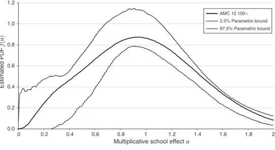
Figure 2 presents estimated distributions of school effects from the data on SAT/ACT high-scorers. The estimated PDF in the top part of the figure has one clear difference from the PDF of the AMC school effects: the distribution is much closer to being symmetric about the u = 1 mean whereas the AMC distribution was skewed to the right. One implication is that there are significantly fewer (14 percent versus 32 percent) schools that are more than 50 percent below average in production of high scores on the SAT/ACT than there are at producing high scores on the AMC. A second striking difference is apparent in panel B: the SAT/ACT distribution has a much thinner upper tail. In the SAT data, only 2 percent of schools are estimated to produce high-scorers at more than twice the average rate, and just 0.02 percent are estimated to produce high-scorers at more than five times the average rate. This contrasts with our earlier estimates that 11 percent of schools that were estimated to produce AMC 12 high-scorers at more than twice the average rate and 1.0 percent 37 Recall that we prioritize SAT scores in this calculation, counting a student who took both exams as having a perfect score if and only if he or she had a perfect score on the math portion of the SAT reasoning test.
at more than five times the average rate. We interpret this contrast as suggesting that the thick upper tail in the AMC 12 school effects distribution is not primarily due to differences in unmeasured student characteristics.
The estimated coefficients on the demographic variables are generally quite similar in the SAT/ACT and AMC estimations, and the former are again similar regardless of whether the coefficients are obtained from negative binomial regres-sion, shown in the fourth column of Table 3, or from our semiparametric estimation, shown in the fifth column. The fact that observed demographics affect the AMC and SAT regressions similarly suggests that unobserved demographic differences may
0.0 0.2 0.4 0.6 0.8 1.0 1.2 0 0.2 0.4 0.6 0.8 1 1.2 1.4 1.6 1.8 2 Estimated PDF f( u)
Multiplicative school effect u
Panel A. Distribution of school effects: students with perfect scores on the SAT/ACT
0.90 0.91 0.92 0.93 0.94 0.95 0.96 0.97 0.98 0.99 1.00 2 3 4 5 6 7 8 Estimated CDF F( u)
Multiplicative school effect u Panel B. Detail on CDF in the upper tail
AMC 12 100+ 2.5% Parametric bound 97.5% Parametric bound AMC 12 100+ 2.5% Parametric bound 97.5% Parametric bound
also have similar effects in the two regressions. Assuming this to be the case, the fact that the estimated α ̂ in the SAT/ACT regression is so much smaller than that in the AMC regression would imply that at most 32 percent of the variance in the AMC school effects is due to unobserved demographic differences. We regard this as a conservative bound because the SAT/ACT school effects reflect more than demo-graphic differences—we assume that there are idiosyncratic differences in how well schools prepare students for the SAT/ACT—and these will be part of what is cap-tured by the SAT/ACT school effects.
C. Unobserved Demographic Differences: Evidence from Gender Differences The effects of schools on female students with high math ability are of indepen-dent interest given the underrepresentation of women in mathematical and techni-cal fields. Data on the female high-scorers also provide another potential source of information into whether heterogeneous outcomes are driven by unobserved demo-graphic differences: differences such as whether a district has many parents with PhDs should be similarly relevant to male and female students (provided there are not large differences in how parents of high-ability girls and boys choose where to live). A number of plausible explanations could be given for why there might be more agglomeration of high-achieving girls. For example, the dispersion of school effects would be larger for girls if there is variation in how encouraging /discourag-ing schools are toward girls independent of a general school-quality effect. Or peer effects could be more important for girls. Or the rigor of a school’s classes might be more important for girls because they are less liable to complain or take supplemen-tary online classes.
The last column of Table 3 reports coefficient estimates from a negative binomial regression with a count of the number of female students scoring at least 100 on the AMC 12 as the dependent variable. Note that the estimated variance of the unob-served school effects, α ̂ of 0.95 (standard error 0.29) whereas it was 0.73 (standard error 0.08) when we examined high-scoring students of either gender. This indicates that there may be more underlying variation in the rate at which different schools are producing high-achieving girls. The substantial noise in the variance estimates from the girls-only sample, however, is such that we cannot say whether the difference in variances is significant.
VI. Mechanisms behind the School Effects
In the preceding sections we argued that a substantial portion of the idiosyncratic differences in the rates at which seemingly similar schools produce high-achieving math students are due to some sort of environmental differences. In this section we present several additional analyses designed to provide insight into what may be leading to these differences.
A. Effects on High-Achieving Students or Generally Strong Math Programs? The fact that a school produces many high-achieving students need not imply that the school’s environment particularly benefits high-achieving students: it could be
that the school just has a generally strong math program. If, for example, the math program at school i raises the score of each student j from θ j to θ j + Δ i , then a school with a larger Δ i will have more students scoring above any particular threshold.
To explore whether this appears to be a large part of what is going with our AMC results, we obtained data on the average math SAT/ACT score for students within each school, which we think of as reflecting the general quality of the school’s math program (as well as observed and unobserved demographics). We then repeated our negative binomial regressions of the number of students scoring at least 100 and at least 120 on the AMC 12 on the same demographics as before plus two additional variables: the average SAT/ACT score in the school and the SAT/ACT participa-tion rate. We find that the added variables only moderately reduce the estimated variance of the school effects. In the AMC ≥ 100 regression the estimated variance α ̂ drops from 0.73 (standard error 0.08) to 0.57 (standard error 0.07). In the AMC ≥ 120 regression the estimated variance α ̂ drops from 2.18 (standard error 0.50) to 1.60 (standard error 0.41).
We also perform a similar exercise in our regressions examining counts of stu-dents with perfect SAT/ACT scores.38 In the SAT/ACT scores, including this
measure of the general quality of the math program reduces the unobserved het-erogeneity nearly to zero; the estimated variance α ̂ drops from 0.23 (standard error 0.03) to 0.07 (standard error 0.02).
If one thinks of the difference between the α ̂ estimated from the AMC data and the α ̂ estimated from the SAT/ACT data as a conservative estimate of the vari-ance in the school effects that controls for both observed and unobserved demo-graphic differences, then the finding of this section is that this difference is 0.50 ( = 0.73 − 0.23 ) when one does not control for the school-average SAT score and also 0.50 ( = 0.57 − 0.07 ) when one does.39 We conclude that a substantial
por-tion of the “school effects” we have reported seems to be due to factors that differ-entially impact high-achieving students.
B. Peer Effects or Differences in School Quality?
Although we have sometimes described our estimated “school effects” as reflect-ing the heterogeneous rates at which schools produce high-scorers, it is more accurate to describe them as a quantification of the excess agglomeration of high-achieving students. Agglomeration will occur if there is unobserved heterogeneity in school “quality.” But it will also be present if there are peer effects among high-achieving students. In this section, we provide a formal nonidentification result, noting that one cannot distinguish peer effects from school quality differences using data on a single cross section; we then show that a calculation using data from multiple years
38 The SAT/ACT participation rate is already included in the controls, so in this exercise we simply add mean SAT/ACT score as a covariate.
39 This comparison is essentially unchanged when we include richer controls for school-average SAT score and participation. The estimated variance α ̂ in the AMC ≥ 100 regression drops from 0.57 (standard error 0.07) when only linear controls are used to 0.56 (standard error 0.07) when cubic polynomials of mean SAT/ACT and partic-ipation, plus an interaction between mean SAT/ACT and participation, are included; the equivalent change in the SAT/ACT high-scorers regression is from 0.07 (standard error 0.02) to 0.04 (standard error 0.01).
suggests that a portion of the school effects we have found are due to peer effects, but that a larger portion is not.
The impossibility of distinguishing peer effects from school-quality differences can be formalized using standard results on the binomial distribution. First, consider a model with no peer effects in which schools differ in unobserved quality (which is captured by a gamma-distributed random variable):
MODEL 1: Suppose the count of high-scorers Y i ∼ Poisson ( λ i ) with λ i = e X i β u
i , where u i ∼ Γ
(
_ α1 , _α1)
.40Second, consider a model with no unobserved heterogeneity u i in school qual-ity, but with peer effects between high-achieving students. Specifically, consider a model in which high-scorers are produced in two ways: the school directly pro-duces high-scoring students at a Poisson rate; and high-scorers produce additional high-scorers via an infection-style dynamic.
MODEL 2: Suppose a school directly produces high-scoring students at Poisson
rate λ ( X i ) during the time interval [0, 1] . Suppose that in each subinterval (t, t + dt) , each high-scoring student then present produces another high-scoring student with probability g ( X i ) dt . Let Y i be the number of high-scoring students at t = 1 .
The two models are well known to produce counts that follow the negative bino-mial distribution.41 As a result, we cannot distinguish between the two models given
a dataset containing a single observation on each school. Conceptually, the argu-ment is similar to Ellison and Glaeser’s (1997) argument that unobserved compara-tive advantages and spillovers can lead to equivalent geographic concentration. PROPOSITION 1: The distribution of Y i | X i under Model 1 with parameters (α, β)
is identical to the distribution of Y i | X i under Model 2 if the direct production rate is
λ( X i ) = __α1 log(1 + α e X i β ) and the peer infection rate is g ( X i ) = αλ ( X i ) .
While the peer effects formulas may seem complicated at first, one can think of them as saying that it is the ratio of the peer infection rate g (x) to the direct pro-duction rate λ (x) that determines the magnitude α of the excess variance (relative to what one would expect with only direct production). Using the approximation log (1 + y) ≈ y , one can think of the formula for the direct production rate as λ( X i ) ≈ e X i β , which is the same functional form as in the unobserved heterogeneity model with the unobserved component set equal to its mean.
A model in which there are both school-quality differences and peer effects of the form above will not produce an exact negative binomial distribution, but the excess variance will still be related to the amount of heterogeneity and the strength of the peer effects in a similar manner. Formally, consider a hybrid model in which
40 The density of the assumed distribution of the u
i is f (u) = (1/α) 1 __α e − 1 __α u u 1 __α −1/Γ (1/α) . 41 In Model 1, Y i ∼ N B ( 1__α , α e X i β ________ 1+α e X i β ) . In Model 2, Y i ∼ NB ( _____λ ( X g ( X i ) i ) , 1 − e −g( X i )
) . See Boswell and Patil (1970, Section 8.2) or Karlin (1966, p. 345) for proofs.