Publisher’s version / Version de l'éditeur:
Vous avez des questions? Nous pouvons vous aider. Pour communiquer directement avec un auteur, consultez la
première page de la revue dans laquelle son article a été publié afin de trouver ses coordonnées. Si vous n’arrivez pas à les repérer, communiquez avec nous à PublicationsArchive-ArchivesPublications@nrc-cnrc.gc.ca.
Questions? Contact the NRC Publications Archive team at
PublicationsArchive-ArchivesPublications@nrc-cnrc.gc.ca. If you wish to email the authors directly, please see the first page of the publication for their contact information.
https://publications-cnrc.canada.ca/fra/droits
L’accès à ce site Web et l’utilisation de son contenu sont assujettis aux conditions présentées dans le site LISEZ CES CONDITIONS ATTENTIVEMENT AVANT D’UTILISER CE SITE WEB.
Technical Report; no. CHC-TR-059, 2009-01-01
READ THESE TERMS AND CONDITIONS CAREFULLY BEFORE USING THIS WEBSITE.
https://nrc-publications.canada.ca/eng/copyright
NRC Publications Archive Record / Notice des Archives des publications du CNRC :
https://nrc-publications.canada.ca/eng/view/object/?id=3c76ab57-c611-473d-8905-74d625b75329 https://publications-cnrc.canada.ca/fra/voir/objet/?id=3c76ab57-c611-473d-8905-74d625b75329
Archives des publications du CNRC
For the publisher’s version, please access the DOI link below./ Pour consulter la version de l’éditeur, utilisez le lien DOI ci-dessous.
https://doi.org/10.4224/20178992
Access and use of this website and the material on it are subject to the Terms and Conditions set forth at
Numerical simulations of ice thickness redistribution and ice drift in the Gulf of St. Lawrence
Numerical Simulations of Ice Thickness
Redistribution and Ice Drift in the Gulf of St.
Lawrence
Ivana Kubat and Mohamed Sayed
Technical Report CHC-TR-059
Numerical Simulations of Ice Thickness Redistribution
and Ice Drift in the Gulf of St. Lawrence
Ivana Kubat and Mohamed Sayed Canadian Hydraulics Centre National Research Council of Canada
Ottawa, Ont. K1A 0R6 Canada
Technical Report CHC-TR-059
ABSTRACT
Canadian Hydraulics Centre of National Research Council of Canada (NRC-CHC) in collaboration with Canadian Ice Service (CIS) of Environment Canada developed an ice forecasting model. Development of this model was initiated to respond to CIS navigation requirements for shipping and navigation in Canadian Arctic. The ice conditions in Canadian Arctic Archipelago are unique due to presence of multi-year ice, ridging, rafting, formation and collapse of ice bridges in the narrow and converging channels, leads opening, and ice pressure build up. Since ice thickness redistribution due to deformation of ice cover is an essential component of high resolution ice forecasting, a parameterization of all the complex processes must be used in order to account for thickness redistribution and lead openings.
The NRC-CHC ice forecasting model deals with these processes through thickness distribution model. That model is an important component of the ice forecasting model. It accounts for continuous evolution of ice thickness and concentration and for the transfer from level to ridged ice. Convergence and shear deformation of the ice cover are considered to transfer part of the level ice into ridged ice. This report presents validation of the NRC-CHC ice thickness redistribution model with field data. The results show that the field observations and model predictions are in a good agreement and that model simulations were able to predict deformation and drift of the sea ice.
TABLE OF CONTENTS ABSTRACT... 1 TABLE OF CONTENTS... 3 LIST OF FIGURES ... 5 LIST OF TABLES ... 7 1.0 INTRODUCTION ... 9
2.0 THE ICE DYNAMICS MODEL... 11
3.0 THICKNESS REDISTRIBUTION MODEL ... 12
4.0 MODEL VALIDATION ... 13 4.1 Event Selection ... 14 4.2 Model Initialization... 15 4.3 Test Results ... 19 5.0 CONCLUSIONS... 27 6.0 ACKNOWLEDGEMENTS ... 28 7.0 REFERENCES ... 28
LIST OF FIGURES
Figure 1 Map of the Gulf of St. Lawrence... 13
Figure 2 Gulf of St. Lawrence: ice conditions before February 2004 storm (photos are courtesy of Dr. Simon Prinsenberg) ... 14
Figure 3 Gulf of St. Lawrence: ice conditions after February 2004 storm (photos are courtesy of Dr. Simon Prinsenberg) ... 14
Figure 4 Ice Chart Ice conditions February 16, 2004 ... 16
Figure 5 The Egg Code Description ... 16
Figure 6 Ice thickness calculated from the February 16, 2004 CIS ice chart. The red square indicates the area for which the results are shown in following Figures. ... 16
Figure 7 Two week time series of 3-hourly meteorological data from CMC’s high-resolution prognostic model for southern Gulf of St.Lawrence, grid point at 63°W and 47°N (Prinsenberg, 2006)... 17
Figure 8 Beacon drift trajectory. Red rectangle specifies the area with the field measurements used in the model... 18
Figure 9: CIS regional ice chart issued on February 23, 2004, 7 days into the run... 20
Figure 10 CIS daily ice chart issued on February 23, 2004, 7 days into the run. The red rectangle marks the area for which the results of the model output are presented in Figures 11 to Figure 18. The model was run the entire area of the Gulf of St.Lawrence. ... 20
Figure 11 Mean Ice Thickness after 7 days ... 21
Figure 12 Ice Concentration in tenths after 7 days ... 21
Figure 13 CIS daily ice chart issued on February 25, 2004, 9 days into the run. The red rectangle marks the area for which the results of the model output are presented... 22
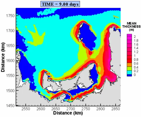
Figure 14 Mean Ice Thickness after 9 days ... 22
Figure 15 Ice Concentration in tenths after 9 days ... 23
Figure 17 Ridged Ice Concentration in tenths after 9 days... 24 Figure 18 Ice Pressure after 9 days ... 24 Figure 19 Ice thickness histograms of pack ice around beacon 26370 on February 16,
2004 ... 25 Figure 20 Ice thickness histograms of pack ice around beacon 26370 on February 24,
2004 ... 25 Figure 21 Ice thickness histograms of the ice input into the model (i.e. representing day 1 – February 16, 2004) ... 26 Figure 22 Ice thickness histogram of ice predicted by after 8 days (i.e. February 24, 2004
... 26 Figure 23 Trajectories of BIO beacon 26370 and a particle representing the location
LIST OF TABLES
Table 1 The values for different ice types used as input parameter in the model... 15 Table 2 Numerical parameters used in the simulation... 18
Numerical Simulations of Ice Thickness Redistribution
and Ice Drift in the Gulf of St. Lawrence
1.0 INTRODUCTION
The essential component of ice forecasting is modeling ice thickness redistribution due to the deformation of the ice cover. Several processes such as rafting, ridging and rubble pile-up contribute to thickness build-up. Also leads may open or close as the ice cover deforms. A parameterization of all those complex processes must be used in order to account for thickness redistribution at the relatively large length scales of relevance to forecasting models.
The basis for most recent models has been the formulation of Thorndike et al (1975). This approach employs probability distribution functions to express the likelihood of ice thickness falling into certain categories (i.e. within certain intervals) and to describe the transfer of ice between thickness categories. The transfer functions are derived from the continuity and energy conservation equations, and through some arbitrary assumptions concerning plausible trends for thickness changes. A number of subsequent models included different implementations of the Thorndike et al (1975) model. For example, Hibler (1979) introduced a two-category version, where one category represented ice and the other category represented open water. Flato and Hibler (1995) introduced a more elaborate formulation with separate thickness distribution functions for ridged and level ice. More recently, Bitz et al (2001) introduced a new Lagrangian formulation to obtain the evolution equation of the ice thickness.
Another approach for characterizing ice cover thickness was developed by Pritchard and Coon (1981). In this approach the ice cover consists of open water (including new ice), thin, flat, and rubbled ice. Thickness redistribution between different categories is addressed in a way that the minimum and maximum thickness, which defines each ice type, change with time in order to account for thermal growth.
Recently, a number of models departed from using discrete thickness categories. Instead of that the models take into account the distribution of thickness between level and ridged ice. First such a model was introduced by Shinohara (1990). He considered that the work done by deforming level ice is proportional to the increase of the potential energy of ridged ice. Gray and Morland (1994) introduced a rigorous derivation for a parameterization of thickness distribution. They considered the transfer from level ice (which they labeled as “coherent”) to deformed ice. Their model keeps track of the area concentration and mean thickness of the level and deformed ice. The proposed formulations account for thickness and concentration changes in response to ice cover deformation. That approach was the basis for further development by Shulkes (1995), and Gray and Killworth (1996). Hapaala (2000) extended that approach by considering several types of ice: level, rafted, ridged, and rubbled.
The present work follows the general approach where evolution of the thickness and concentration of the ice cover due to convergence and shear deformation is considered. Thorndike’s et al (1975) approach was not adopted for the new model for a number of reasons. It requires computationally demanding operations to keep track of thickness evolution in many categories (typically 25 or more categories). Thickness evolution equations are based on somewhat arbitrary and complex assumptions, and finally no distinction is made between level and ridged ice. An approach based on keeping track of the mean thickness and concentration of ridged and level ice was therefore chosen. Testing of available models, however, showed problems with various formulations. For example, the model of Gray and Morland (1994) was tested, starting from a relatively small concentration of ridged ice thickness under compression. The results showed unrealistically progressive reduction of the ridged area and increase in ridged ice thickness. Naturally, the expected outcome should display an increase, instead of reduction, of ridged ice area. The model of Hapaala (2000) displayed another problem. It predicted unrealistic changes to level ice thickness.
Recently Savage (2002) introduced a model that includes new expressions for the transfer from level to ridged ice. That model was aimed at enhancing the operational ice forecasting model under development by the Canadian Ice Service (CIS). Savage in the thickness redistribution model goes through rigorous derivations of evolution equations and avoids many arbitrary assumptions in the past models. Basically in his model there is no need for keeping track of many categories. The ice cover is represented by two parts: level ice and ridged ice. Each part is assigned a concentration (area coverage) and a thickness. Convergence and shear deformation of the ice cover are considered to transfer part of the level ice into ridged ice. The approach of the model is based on taking into account conservation of ice mass and balance of energy of mechanical deformation and potential energy required to increase the thickness of ridged ice. Formulas were derived to keep track of the evolution of the concentration of thickness of level ice and ridged ice. Thus, as the ice cover deforms, the model determines the change in concentration of level ice and ridged ice, as well as the increase of ridged ice thickness. Note that level ice thickness remains unchanged in the absence of thermodynamic growth and melt. Initial tests of the model of Savage (2002) indicated that the results are reasonable under several deformation scenarios.
The model of Savage (2002, 2008) deals with thicknesses and concentrations in the context of the Particle in Cell (PIC) approach. In this approach each particle carries attributes describing ice properties. These PIC particles occupy relatively small areas and the properties such as thicknesses and concentrations vary from particle to particle, depending on the history of the forcing that each of the particles was subjected to. When a larger region that contains a number of PIC particles is examined, things like ice thickness distribution functions that are built into other models such as that of Thorndike et al (1975) can be recovered.
The new model was initially tested under a wide range of idealized deformation conditions such as uniaxial compression (ice flow against the shoreline), shear (ice flow along the shoreline), and combined shear and compression Kubat et al. (2004). These
mean thickness for the ridged ice and level ice. In addition the thickness redistribution formulation and the flow of the ice through converging channels has been examined (Kubat et al. 2005, 2006 and 2007). Only thickness evolution due to mechanical deformation is considered here. Thermodynamic effects are not included. The model has been validated with the field measurements in the Gulf of St. Lawrence. This paper presents results of such testing. The results indicate that the model produces appropriate behaviour and trends.
2.0 THE ICE DYNAMICS MODEL
The model has been described in a number of past publications, therefore only a brief overview is given in this paper. Detailed description of the model can be found in Sayed and Carrieres (1999); and Sayed et al. (2002). The dynamics model solves the equations of balance of mass and momentum. The momentum equation considers the forces acting on the ice cover due to air and water drag, Coriolis force, and water surface tilt. In addition, constitutive equations are needed to relate the stresses and strain rates.
The CIS ice forecasting model consists of a number of components. The important component of the model is Particle in Cell (PIC) approach to model ice advection. In that approach, an ensemble of discrete particles represents the ice cover. The particles are assigned several attributes such as thickness and concentration of both level and deformed ice, position, velocity, and acceleration. The particles are advected in a Lagrangian manner. At each time step particles are moved to their new position. Their attributes are then mapped to the underlying computational grid. A bilinear interpolation function is used to map variables between the particles and the fixed Eulerian grid (Sulsky et al., 1994). The momentum and continuity equations are solved over the grid. Velocities are determined by interpolating node velocities of the grid. The area and mass of all particles within each grid cell are then averaged to update the thickness and ice concentration at the Eulerian grid nodes. The resulting accelerations and solids volume fractions are mapped back to the particles. Particles are then advected. Throughout each process the PIC approach keeps track of the history of each particle.
For rheology and constitutive equations, the Hibler’s (1979) viscous plastic formulation is used. In this formulation viscosity coefficients are chosen to describe an elliptic plastic yield envelope. Strength of the ice cover also follows Hibler’s formulation, in which strength depends on ice thickness and concentration as well as a strength parameter P*. The momentum equations are solved using the semi-implicit method of Zhang and Hibler (1997). This method is also used to update pressures on the grid. Another important component of the CIS ice forecasting model is thickness redistribution model described in the following section.
3.0 THICKNESS REDISTRIBUTION MODEL
The thickness redistribution model of Savage (2002, 2008) provides a parameterization for the dependence of ridging and lead opening processes on deformation. The model accounts for the continuous evolution of the thickness and concentration of ice without resorting to discrete categories. The equations of the thickness redistribution model are briefly listed here. Further discussions and testing of the model can be found in Kubat et al. (2004). Detailed description of the thickness redistribution model can be found in Savage, 2008.
The area fraction of the ice cover, A is divided into two area fractions, Au and Ar, representing the level (or undeformed) ice and ridged ice, respectively. Thus, the total area fraction of the ice cover can be expressed as
r u A A A= + (1) r r u uh A h A h A = + (2)
where the subscripts u and r refer to level (or undeformed) ice and ridged (or deformed) ice, respectively. Evolution equations for the thickness and area fraction are derived by considering the continuity and energy balance equations. Those equations depend on the velocity divergence, η, and a redistribution function, ψ. The divergence is given by
2 1 • • + =e e η (3)
where and , are the principal strain rates. The redistribution function is
(
)
[
]
⎥ ⎥ ⎥ ⎥ ⎥ ⎦ ⎤ ⎢ ⎢ ⎢ ⎢ ⎢ ⎣ ⎡ ⎥ ⎥ ⎥ ⎥ ⎦ ⎤ ⎢ ⎢ ⎢ ⎢ ⎣ ⎡ ⎟ ⎠ ⎞ ⎜ ⎝ ⎛ − + ⎟ ⎠ ⎞ ⎜ ⎝ ⎛ + − ⎟ ⎠ ⎞ ⎜ ⎝ ⎛ + − − = • • • • • • 2 / 1 2 2 2 1 2 2 1 2 1 1 exp 2 1 e e e e e e e A C A ψ (4)where the constant C is used in the common expression for ice pressure.
The resulting evolution equations are summarized as follows. The rate of change of the area fraction of ridged and level ice (Ar and Au, respectively), total area fraction A, ridged
ice thickness hr, and mean ice thickness h, are:
(
β)
ψ η= − + r 1 r A t D A D (5)u t D ψ η= + A t D A D (7) ⎥ ⎦ ⎤ ⎢ ⎣ ⎡ − ⎟⎟ ⎠ ⎞ ⎜⎜ ⎝ ⎛ − = 1 1 r u r r r h h A h t D h D ψ β (8) A h t D h D ψ − = (9)
The parameter β was derived by considering that the ratio of level ice thickness to ridged ice thickness, hu/hr, reaches an asymptotic value (see for example Hopkins, 1998). The
resulting expression is 2 / 1 7 . 16 7 . 16 u h − = β (10)
The evolution equations (equations 5 to 9) are solved for each PIC particle
4.0 MODEL VALIDATION
A number of simulations were done to examine performance of the model. The model has been examined with field data obtained from the Gulf of St. Lawrence. Figure 1 shows the map of the Gulf of St. Lawrence.
Magdalen Islands Summer route
Winter route
4.1 Event Selection
The area north of Prince Edward Island (PEI) and in the vicinity of the Magdalene Island represents a region where vessels are often trapped in pressured and ridged ice. It is therefore important to provide a reliable forecast on ice conditions in this region. Field data and measurements are a means for validating accuracy of the forecast. Bedford Institute of Oceanography (BIO) uses satellite-tracked ice beacons and helicopter-borne electromagnetic sensors to measure ice drift, ice thickness, and surface ice roughness. During February and March of 2004 BIO collected ice drift and ice thickness data in the Gulf of St.Lawrence North of Prince Edward Island (PEI) to study ice thickness evolution and ice drift behaviour in response to winter storms in that region (Prinsenberg et al, 2006). BIO deployed five beacons during this program (Van der Baaren, 2004). Only two beacons, 26370 and 26386, survived an unusually severe winter storm on February 19, 2004. During this storm high ridges were formed. Data collected from beacon 26370 were used for the validation of the model. The beacon was deployed on February 16, 2004 on 60 cm thick ice floe at 46.6°N and 63.08°W. Figure 2 shows the ice conditions before the storm and Figure 3 after the storm. An arrow in the first picture of Figure 3 points to a large long ridge that was formed during the storm; the second picture in Figure 3 zooms on a ridge formed during the storm.
Figure 2 Gulf of St. Lawrence: ice conditions before February 2004 storm (photos are courtesy of Dr. Simon Prinsenberg)
Figure 3 Gulf of St. Lawrence: ice conditions after February 2004 storm (photos are courtesy of Dr. Simon Prinsenberg)
4.2 Model Initialization
Test 1
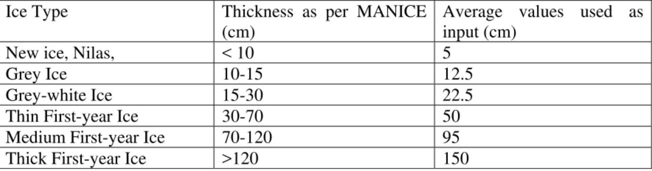
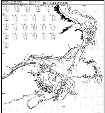
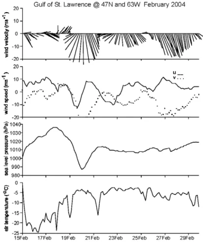
Two tests were run to examine the model. In the first test the ice conditions were obtained from the Canadian Ice Service (CIS) digital ice chart issued for the Gulf of St. Lawrence on February 16, 2004. The corresponding jpg image for this digital ice chart is shown in Figure 4. The land boundary of the Gulf of St.Lawrence was masked according to the land boundary provided on CIS Ice Charts using the ArcView GIS software. This was done in order to distinguish between land and water. The boundaries of ice regimes (region with the same ice thickness and concentration) defined in digital CIS Ice Chart as polygons were imported into the ArcView and intersected with the land mask. The area was divided into 5 km grid cells that were used in the model. The ice conditions in each ice regime are described by the egg code. The egg code is explained in Figure 5. Coding of the ice charts is described in detail in CIS MANICE (MANICE, 2005). Each ice type represents a range of ice thickness. The average values for each thickness range were calculated and taken as the initial ice thickness (Table 1). Only first-year ice is present in the Gulf of St. Lawrence. The weighted averages calculated from the ice concentration given by the regional digital ice chart and the averaged ice thickness were used as the initial input conditions in the model. Figure 6 shows the regions coloured according to weighted ice thickness calculated from the February 16, 2004 CIS digital regional ice chart. The model was run for the Gulf of St. Lawrence for the area between 45° to 52° N and 55° to 70° W. The red square in Figure 6 marks the area zoomed on Prince Edward Island and Magdalene Island for which the results are shown in Figure 11 to Figure 18. The wind speed and direction were obtained from the Canadian Meteorological Centre (CMC) high-resolution prognostic model for southern Gulf of St. Lawrence. Data collected at a grid point at 63°W and 47°N, closest to the location of the beacon 26370 deployment, were used. Figure 7 shows the wind, pressure and direction for the last two weeks in February.
Table 1 The values for different ice types used as input parameter in the model
Ice Type Thickness as per MANICE
(cm)
Average values used as input (cm)
New ice, Nilas, < 10 5
Grey Ice 10-15 12.5
Grey-white Ice 15-30 22.5
Thin First-year Ice 30-70 50
Medium First-year Ice 70-120 95
Figure 4 Ice Chart Ice conditions February 16, 2004
Figure 5 The Egg Code Description
Modeled area
Figure 6 Ice thickness calculated from the February 16, 2004 CIS ice chart. The red square indicates the area for which the results are shown in following Figures.
Figure 7 Two week time series of 3-hourly meteorological data from CMC’s high-resolution prognostic model for southern Gulf of St.Lawrence, grid point at 63°W and 47°N (Prinsenberg, 2006)
The water currents were obtained from BIO 3D model. The currents are modelled estimates for the actual current at 5m depth at the location 63.08°W and 46.6°N. They include tides and atmospheric forcing, and fresh water run off. The tides are the ocean response to periodic elevation forcing specified along the boundaries. The atmospheric forcing is the 6 hour National Centres for Environmental Predictions (NCEP) reanalysis. Fresh water run-off includes monthly amounts for major rivers. For the purpose of our validation the currents were output every hour. Since the time step of the forecasting model was 5 minutes, the water current input into the forecasting model was constant over 12 time steps and updated every 13th time step with the new hourly output from the BIO model. Coriolis force was set to 0. Values of other run parameters are listed in Table 2.
Table 2 Numerical parameters used in the simulation Air
Air drag coefficient 0.002
Air density 1.3 kg m-3
Water
Water drag coefficient 0.005
Water density 103 kg m-3
Ice
Ice strength, P* 104 Pa
Ice density 910 kg m-3
Elliptical yield envelope axes ratio, e
2
Constant C 20
Run
Time step 5 minutes
Grid cell size 5 km
Duration 9 days
Test 2
In the second case, we focused on the area North of Prince Edward Island where the beacon 26370 was deployed and the actual ice conditions were measured (Figure 8). Field observed ice conditions are more detailed and accurate than those obtained from the ice charts, which interpret the ice conditions from radar imagery. The initial ice conditions input into the model for the area marked by red rectangle were modified to agree with the field measurements. The initial ice conditions for the rest of the Gulf of St. Lawrence were obtained from the CIS digital ice chart. The rest of the run parameters were the same as those in Test 1. The data output by the forecasting model were compared with BIO data collected by satellite-tracked ice beacon and helicopter-borne electromagnetic sensor. The BIO data represent high quality and high resolution dataset, therefore are ideal for examining accuracy of the model.
Figure 8 Beacon drift trajectory. Red rectangle specifies the area with the field measurements used in the model.
4.3 Test Results
Test 1
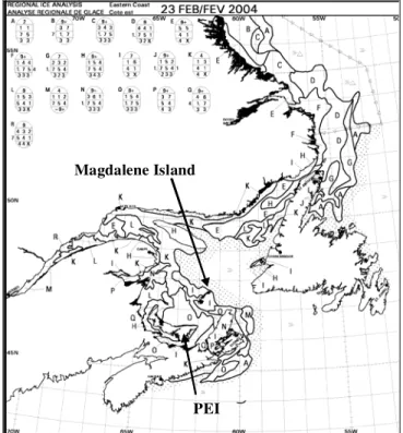
The ice conditions from February 16, 2004 to February 25, 2004 were simulated by the model and compared with the ice conditions given by the CIS ice charts. Two types of ice charts were used in the analysis. Regional digital ice charts for the input and both regional and daily ice charts for comparing the model output. Regional ice charts are not as detail as the daily ice charts. They are issued on weekly basis, however they provide information on ice conditions in digital format which is needed as the input into the model. When the regional chart is produced for an area where daily ice charts are available, the daily ice charts are used as a basis of the regional chart. Details such as strips and patches, and small ice areas are removed from the chart. Figure 9 shows CIS regional ice chart issued on February 23, 2004, 7 days into the run. Figure 10 shows CIS daily ice chart issued on the same day, February 23, 2004. The red rectangle marks the area for which the results of the model output are presented in the following Figures. Figure 11 shows mean ice thickness output by the model. The polygons in Figure 11 represent the ice regimes given by the regional ice chart. Since the daily ice charts are not issued in digital format we could not plot the polygons of the ice regimes for daily ice chart, therefore used the polygons from digital ice chart. Figure 12 presents total ice concentration output by the model. As can be seen there is a good agreement between the model output and the ice conditions presented on the daily ice chart issued for February 23, 2004 (Figure 10). For example a very low ice concentration and ice thickness East of the Magdalene Island or West of the South tip of the Magdalene Island, low ice concentration and ice thickness in vicinity of PEI, or higher ice thickness in a small region westward from the south tip of the Magdalene Island and against the cost of Cape Breton. Figure 13 shows daily ice chart issued on February 25, 2004, 9 days into the run. Only daily ice chart is available for this day. Figure 14 and Figure 15 show mean ice thickness and total ice concentration, respectively. There is again a good agreement between the ice chart ice conditions and ice conditions output by a model. In addition to mean ice thickness and ice concentration the model predicts thickness of ridged ice, concentration of ridged ice and pressure build up. These can be seen in Figure 16 to Figure 18, respectively. These figures show higher concentration and build up of ridged ice against the islands and in the vicinity of the coastline. The same stands for ice pressure build up.
The ice conditions described on the CIS ice charts are based on ice observations interpreted from radar imagery. For further validation of the model we focused on the area for which high quality field data measurements were available. These data give more accurate ice conditions input into the model. Results of such validation are described under Test 2.
Magdalene Island
PEI
Figure 9: CIS regional ice chart issued on February 23, 2004, 7 days into the run
Magdalene Island
Modeled area
Figure 10 CIS daily ice chart issued on February 23, 2004, 7 days into the run. The red rectangle marks the area for which the results of the model output are presented in Figures 11 to Figure 18. The model was run the entire area of the Gulf of St.Lawrence.
Figure 11 Mean Ice Thickness after 7 days
Magdalene Island
Modeled area
Figure 13 CIS daily ice chart issued on February 25, 2004, 9 days into the run. The red rectangle marks the area for which the results of the model output are presented.
Figure 15 Ice Concentration in tenths after 9 days
Figure 17 Ridged Ice Concentration in tenths after 9 days
Test 2
Test 2 examined the performance of the model using the field data. For this purpose the initial ice conditions input into the model were modified to agree with the field measurements obtained north of PEI. Figure 8 presents a drift trajectory of the beacon 26370 deployed on February 16th, 2004 (Julian Day 47) which was simulated by the forecasting model. Red rectangle in Figure 8 shows the area for which the ice thickness distribution histograms were generated. Figure 19 and Figure 20 show ice thickness distribution measured before the storm (February 16) and after the storm (February 24), respectively. Figure 21 and Figure 22 show ice thickness distribution obtained from the model. Figure 21 represents the ice conditions on February 16 and Figure 22 conditions after the storm on February 24. As can be seen there is a good agreement between the field measurements and the model output. The model output gives the same trend and the same peak magnitude as the field measurements, the same location of the peak of distribution, and general trend of distribution.
Figure 19 Ice thickness histograms of pack ice around beacon 26370 on February 16, 2004
Figure 20 Ice thickness histograms of pack ice around beacon 26370 on February 24, 2004
Initial 0% 5% 10% 15% -0.1 1.0 2.0 3.0 4.0 5.0 6.0 Ice Thickness, m No rm al iz e d Fr eq u e nc y
Figure 21 Ice thickness histograms of the ice input into the model (i.e. representing day 1 – February 16, 2004) DAY 8 0% 5% 10% 15% -0.1 1.0 2.0 3.0 4.0 5.0 6.0 Ice Thickness, m No rm al iz e d Fr eq ue nc y
Figure 22 Ice thickness histogram of ice predicted by after 8 days (i.e. February 24, 2004
Figure 23 shows trajectories of beacon 26370 and a particle representing the location where the beacon was deployed. There is 25 km offset between the trajectories on day 2.5 and 17 km offset on day 3.8. This is due to the fact that wind and tidal current inputs did not vary spatially, rather were only time-dependent. Also the initial position of the modeled particle is slightly offset from the initial position where the beacon was deployed. Overall, there is a good agreement between both trajectories. In both cases the beacon and particle stopped after 4 days in the ridged pack ice that got compressed against the PEI.
3.88 3.87 2.51 2.5 Start Model Field
After 4 days beacon stopped in the ridged pack ice compressed against PEI
PEI
Figure 23 Trajectories of BIO beacon 26370 and a particle representing the location where the beacon was deployed
5.0 CONCLUSIONS
The work described in this paper is part of an effort to examine the CIS Ice Forecasting model (ice dynamics model) and its thickness redistribution component. The ice dynamics model is based on a Particle-In-Cell (PIC) approach, where an ensemble of discrete particles represents the ice cover. The attributes of ice cover such as area and thickness, are advected in a Lagrangian manner, which allows keeping a track of the history of ridging and thickness evolution. Ice thickness redistribution component of the CIS ice dynamics model is model on its own. It considers two ice categories: level (undeformed) ice and ridged (deformed) ice. The thickness redistribution model provides a parameterization for the dependence of ridging and lead opening processes on deformation. It accounts for the continuous evolution of the thickness and concentration of ice without resorting it to discrete categories (Savage 2008). Output of the thickness redistribution model predicts the development of thickness and concentration of each category in response to deformation. The model considers the transfer of ice from level to ridged ice due to convergence and shear deformation of the ice cover. The evolution equations in the thickness redistribution model are solved for each PIC particle.
Comparisons with field observations for verification of model prediction were carried out. The ice conditions during the storm in February 2004 in the Gulf of St. Lawrence were simulated and results of two tests were described. The first test simulated a large portion of the Gulf of St.Lawrence. The ice conditions used as input parameters and for validating the model in this test were obtained from the Canadian Ice Service ice charts, which are based on ice observations interpreted from radar imagery. For further validation of the model we zoomed on a smaller area for which high quality field data
measurements were available. In both cases the model was run for 9 days, period representing duration of the storm in February 2004. Model output was compared to corresponding ice charts and field measurements. In both cases the model shows a good performance. In comparison with the ice charts, the model simulated well low ice concentration and ice thickness that was apparent in vicinity of Magdalene and Prince Edward Islands, as well as build up of ice thickness in the modelled area. A distribution of ice thickness over the area north of Prince Edward Island output by the model was in a good agreement with the ice thickness distribution obtained from the field measurements in the same area. Examination of the thickness distribution model proves effectiveness of the model in simulating the process of ice thickness and ice concentration evolution. The comparison between the observations and model predictions confirms that simulations were able to predict deformation and drift of the sea ice.
6.0 ACKNOWLEDGEMENTS
The support of the Panel on Energy Research and Development (PERD) is gratefully acknowledged. Thanks also belong to our colleague Anne Collins for processing CIS digital ice charts and masking the land and boundary conditions, and to Simon Prinsenberg, Joel Chasse and Adam Drozdowski from Bedford Institute of Oceanography (BIO) for providing the field data and modeled currents.
7.0 REFERENCES
Bitz, C.M., Holland. M.M., Weaver, A.J., Eby, M. (2001) “Simulating the ice thickness distribution in a coupled climate model”. J. Geophys. Res., Vol.106, pp. 2,441-2,463. Flato, G.M., and Hibler III, W.D. (1995). “Ridging and strength in modeling the thickness distribution of Arctic sea ice”, J. Geophys. Res., Vol.100 (C9), pp. 18,611- 18,626.
Gray, J.M.N.T. and Morland, L.W. (1994). “A teo-dimensional model for the dynamics of sea ice”. Philos. Trans. R. Soc. London. A, 347, pp 219-290.
Gray, J.M.N.T. and Killworth, P.D. (1996). “Sea ice ridging schemes”. J. Phys.
Oceanogr. Vol. 26, pp. 2,420-2,428.
Haapala, J. (2000). “On the modelling of ice-thickness redistribution”. J. Glaciology. 46, pp. 427-437.
Hibler III, W.D. (1979). “A dynamic thermodynamic sea ice model,” J. Physical
Oceanography, Vol. 9, No. 4, pp. 815-846.
Hopkins, M.A. (1998). “Four stages of pressure ridging.” J. Geophys. Res., Vol. 103 (C10), pp. 21,883- 21,891.
Canadian Ice Service Ice Thickness Redistribution Model,” Proc Int Offshore and Polar
Eng Conf, ISOPE, Toulon, France, May 23-28, pp 855-862.
Kubat, I, Sayed, M, Savage, S, and Carrieres, T. (2005). “Implementation and testing of a thickness redistribution model for operational ice forecasting,” Proc Int Conf on Port and
Ocean Eng under Arctic Conditions, POAC, Potsdam, NY, USA, June 26-30, Vol 2, pp
781-791.
Kubat, I., Sayed, M., Savage, S. and Carrieres, T. (2006) “Flow of ice through converging channels” Proc 16th Int Offshore and Polar Engineering Conf, ISOPE, San Francisco, CA, USA, Vol. 1, pp 577-583
Kubat, I, Sayed, M, Savage, S, and Carrieres, T. (2007). “Flow of ice through long converging channels,” Proc Int Conf on Port and Ocean Eng under Arctic Conditions, POAC, Dalian, China, June 27-30, Vol 2, pp 673-682.
MANICE – Manual of Standard Procedures for Observing and Reporting Ice Conditions, June 2005, Revised Ninth Editions.
Prinsenberg, S.J., Van der Baaren, A., and Peterson, I.K. (2006). ”Ice ridging and ice drift in southern Gulf of St. Lawrence, Canada during winter storms”. Annals of Glaciology Vol. 44: 411-417
Pritchard, R.S., and Coon, M.D. (1981). “Canadian Beaufort sea ice characterization,”
Proc. The 6th Int Conf. On Port and Ocean Eng. Under Arctic Conditions (POAC 81),
Quebec, Canada, July 27-31, Vol II, pp.609-618.
Savage, S.B. (2002). “Two category sea-ice thickness redistribution model,” Report
prepared for Canadian Ice Service, Environment Canada, 373 Sussex Dr, Ottawa, Ontario, Canada, K1A 0H3, March 31, 2002.
Savage, S.B. (2008). “Two Component Sea-Ice Thickness Redistribution Model,” Cold
Regions Science and Technology, Vol.51, Issue 1, pp 20-37.
Sayed, M., and Carrieres, T. (1999). “Overview of a new operational ice forecasting model”, Proc. Int. Offshore and Polar Eng. Conf., ISOPE, Brest, France, May 30- June 4, Vol. II, pp. 622-627.
Sayed, M., Carrieres, T., Tran, H. and Savage, S.B. (2002). “Development of an operational ice dynamics model for the Canadian Ice Service,” Proc. Int. Offshore and
Polar Eng. Conf., ISOPE, Kitakyushu, Japan , May 26-31, pp. 841-848.
Shulkes, R.M.S.M. (1995). “A note on the evolution equations for the area fraction and the thickness of a floating ice cover”. J. Geophys. Res. Vol. 100 (C3). Pp. 5,021-5,024.
Sinohara, Y. (1990). “A redistribution function applicable to a dynamic model of sea ice”, J. Geophys. Res., Vol. 95, pp. 13,423-13,431.
Sulsky, D, Chen, Z, and Schryer, HL (1994). “Particle method for history-dependent materials,” Comput Methods Appl Mech Eng, Vol 118, pp 179-196
Thorndike, A.S., Rothrock, D.A., Maykut, G.A., and Colony, R. (1975). “The thickness distribution of sea ice”, J. Geophys. Res., Vol.80, pp. 4,501-4,513.
Van der Baaren, A., “Satellite-tracked Ice Beacon Program 2004: Gulf of St. Lawrence”
Internal Report prepared for Bedford Institute of Oceanography” pp 46.
Zhang, J and Hibler III, WD (1997). “On an efficient numerical method for modelling sea ice dynamics,” J Geophysical Research, Vol 102, No C4, pp 8691-870