HAL Id: insu-02474168
https://hal-insu.archives-ouvertes.fr/insu-02474168
Submitted on 11 Feb 2020HAL is a multi-disciplinary open access archive for the deposit and dissemination of sci-entific research documents, whether they are pub-lished or not. The documents may come from teaching and research institutions in France or abroad, or from public or private research centers.
L’archive ouverte pluridisciplinaire HAL, est destinée au dépôt et à la diffusion de documents scientifiques de niveau recherche, publiés ou non, émanant des établissements d’enseignement et de recherche français ou étrangers, des laboratoires publics ou privés.
To cite this version:
Maxime Bernard, Philippe Steer, Kerry Gallagher, David Egholm. The effects of ice and hillslope erosion and detrital transport on the form of detrital thermochronological age probability distributions from glacial settings. Earth Surface Dynamics, European Geosciences Union, inPress, �10.5194/esurf-2020-7�. �insu-02474168�
The effects of ice and hillslope erosion and detrital transport on the
form of detrital thermochronological age probability distributions
from glacial settings
Maxime. Bernard
1, Philippe. Steer
1, Kerry. Gallagher
1, David Lundbek. Egholm
21Univ Rennes, CNRS, Géosciences Rennes, UMR 6118, 35000 Rennes, France.
5
2Department of Geoscience, Aarhus University, Aarhus, Denmark. Correspondence: Maxime Bernard (maxime.bernard@univ-rennes1.fr)
Abstract. The impact of glaciers on the Quaternary evolution of mountainous landscapes remains controversial. Although in
situ low-temperature thermochronology offers insights on past rock exhumation and landscape erosion, the methods also suffer from biases due to the difficulty of sampling bedrock buried under glaciers. Detrital thermochronology attempts to bypass this 10
issue by sampling sediments, at e.g. the catchment outlet, that may originate from beneath the ice. However, the age distributions resulting from detrital thermochronology do not only reflect the catchment exhumation, but also the patterns and rates of surface erosion and sediment transport. In this study, we use a new version of a glacial landscape evolution model, iSOSIA, to address the effect of erosion and sediment transport by ice on the form of synthetic detrital age distributions. Sediments are tracked as Lagrangian particles which can be formed by bedrock erosion, transported by ice or hillslope 15
processes and deposited. We apply our model to the Tiedemann glacier (British Columbia, Canada), which has simple morphological characteristics, such as a linear form and no connectivity with large tributary glaciers. Synthetic detrital age distributions are generated by specifying an erosion history, then sampling sediment particles at the frontal moraine of the modelled glacier.
An assessment of sediment transport shows that 1500 years are required to reach an equilibrium for detrital particle age 20
distributions, due to the large range of particle transport times from their sources to the frontal moraine. Next, varying sampling locations and strategies at the glacier front leads to varying detrital SPDFs, even at equilibrium. These discrepancies are related to (i) the selective storage of a large proportion of sediments in small tributary glaciers and in lateral moraines, (ii) the large range of particle transport times, due to varying transport lengths and to a strong variability of glacier ice velocity, (iii) the heterogeneous pattern of erosion, (iv) the advective nature of glacier sediment transport, along ice streamlines, that leads to a 25
poor lateral mixing of particle detrital signatures inside the frontal moraine. Finally, systematic comparisons between (U-Th)/He and fission track detrital ages, with different age-elevation profiles and relative age uncertainties, show that (i) the nature of the age-elevation relationship largely controls the ability to track sediment sources, and (ii) qualitative first-order information may still be extracted from thermochronological system with high uncertainties (> 30 %) depending on erosion pattern. Overall, our results demonstrate that detrital age distributions in glaciated catchments are strongly impacted not only 30
distributions, detrital thermochronology offers a means to constrain the transport pattern and time of sediment particles. However, our results also suggest that detrital age distributions of glacial features like frontal moraines, are likely to reflect a transient case as the time required to reach detrital thermochronological equilibrium is of the order of the short-timescale glacier dynamics variability, as little ice ages or recent glaciers recessions.
1 Introduction
5
Glaciers have left a profound impact on the topography of mountainous landscapes in particular by eroding deep glacial valleys and depositing large volume of sediments in moraines. As glacier dynamics are linked to climate, an active area of research aims to characterize the role of glacial erosion on the dynamics and relief development of mountain belts during the recent Quaternary glaciations (e.g. Zachos et al., 2001; Molnar and England, 1990; Beaumont et al., 1992; Montgomery, 2002;
Brozović et al., 1997; Whipple et al., 2009; Steer et al., 2012; Champagnac et al., 2014). To address these questions, two 10
timescales have typically been considered: a longer timescale (105-106 years) to assess the potential glacial imprint on the
landscape, and a shorter timescale (101-104 years) to understand how ice actually erodes the landscape. For example, some
studies integrated glacial sediment records worldwide and in situ low-temperature thermochronology data, to estimate glacial erosion rates. They showed average erosion rates of 100-103 mm yr-1 on short timescales (103-105 years) and long-term (>106
years) average erosion rates of 10-2-100 mm yr-1 (Hallet et al., 1996; Koppes and Montgomery, 2009; Valla et al., 2011b;
15
Koppes et al., 2015; Bernard et al., 2016).
Herman et al. (2013) used a global compilation of in situ thermochronological data and an inverse approach to infer an increase in erosion rates for all mountain ranges in the Quaternary period. They suggested that this effect is more pronounced for glaciated mountains, suggesting a significant role of glaciation on erosion rates. However, the results of this study have been contested (Willenbring et al., 2016; Schildgen et al., 2018) and the link between the long-term glaciation and an increase of 20
erosion rates is still debated. In situ thermochronology consists of collecting bedrock samples from discrete locations to map thermochronological ages and exhumation rates (e.g., Fitzgerald and Stump, 1997; Valla et al., 2011b, Herman et al., 2013). However, this approach offers a potentially biased assessment of catchment wide exhumation pattern as it is dependent on the spatial bedrock sampling strategy (Ehlers, 2005, Valla et al., 2011a). For example, the age-elevation relationship inferred from in situ thermochronology may not account for young thermochronological ages expected along the valley floor, and buried 25
under the ice (Enkelmann et al., 2009; Grabowski et al., 2013).
In glacial environment, erosion mostly occurs subglacially through abrasion and quarrying (Boulton, 1982; Hallet et al., 1996) or supraglacially (i.e. ice-free areas) through periglacial mechanisms and gravitational processes (Matsuoka and Murton, 2008). These two sources (i.e. supraglacial and subglacial areas), and their contribution to erosion, define the relative proportion of sediments that enter the glacier transport system (Small, 1987). Sediments are transported by glaciers by (i) 30
subglacial water flow through cavity or channel systems (Kirkbride, 2002; Alley et al., 1997; Spedding, 2000), and (ii) by ice internal deformation for sediments incorporated within or above the ice (Hambrey et al., 1999; Goodsell et al., 2005).
Therefore, sampling and analysing these sediments (detrital thermochronology) has the potential to provide a more spatially integrated view of the catchment erosion pattern on short timescales (101-104 years) and thereby a more representative
indication of how ice is eroding the landscape (e.g. Stock et al., 2006; Tranel et. 2011; Ehlers et al., 2015). The detrital sampling protocol focusses on collecting glacial deposits, generally close to the outlet of the catchment (Ruhl and Hodges, 2005; Stock et al., 2006; Falkowski et al., 2016; Glotzbach et al., 2018). A major motivation for detrital sampling is that we 5
can potentially obtain grains from regions inaccessible for bedrock sampling due to ice cover and lack of outcrop or, more pragmatically, logistical considerations (e.g. cost).
Thermochronological age distributions of detrital samples are generally interpreted in terms of synoptic probability density functions (SPDF) (Brewer et al., 2003; Ruhl and Hodges., 2005). Analysis of many glacial catchments has been based on the interpretation of these SPDFs (Stock et al., 2006; Tranel et al., 2011; Avdeev et al., 2011; Thomson et al., 2013). More recently, 10
Enkelmann and Ehlers (2015) and Ehlers et al. (2015) investigated the erosion patterns and the degree of mixing of ice-cored sediments at the terminus of the Tiedemann glacier (Coast Mountains, Canada) using both detrital and in situ low-temperature thermochronology. By comparing the bedrock and detrital age distributions, they inferred that sampling through the terminal moraine is similar to sampling the pro-glacial rivers, supporting the idea of an efficient mixing of glaciated sediments at the glaciers front. The latter result is also consistent with results obtained on the Malaspina Glacier, Alaska (Enkelmann et al., 15
2009; Grabowski et al., 2013). However, the authors pointed out the sensitivity of their results to the relatively high age uncertainties of the data. Furthermore, while the shape of SPDFs is expected to be mainly controlled by the catchment exhumation history, other processes such as grain erosion, transport and deposition are likely to also influence the form of SPDFs. These factors will contribute to the overall integration of the spatially variable products of erosion into the sediment ultimately deposited at the outlet.
20
In this study, we address the effect of sediment transport by the ice and the role of the different source areas (i.e. subglacial and supraglacial) in the shaping of detrital SPDF of thermochronological ages. To this end, we use numerical models simulating the Tiedemann glacier to explore the effect of surface processes, including erosion and transport by the ice, on the detrital SPDFs that we compare with the bedrock age distribution. We take advantage of a new version of the glacial landscape evolution model iSOSIA (for integrated Second Order Shallow Ice Approximation,Egholm et al., 2011) that includes sediment 25
particle tracking. First, we focus on the description of the dynamics of sediment transport within the modelled catchment. Second, we perform three numerical simulations that consider (i) uniform erosion, (ii) glacial-only erosion, and (iii) hillslope-only erosion. These experiments allow us to explore the influence of 1) ice transport and 2) sediment source areas, both subglacial and supraglacial, on the shape of the detrital SPDF. Finally, we consider non-uniform erosion, by letting iSOSIA and its implicit erosion laws control the pattern of erosion. This last experiment allows us to assess the record of such complex 30
erosion processes contained in the shape of detrital SPDFs. For each experiment, we produce synthetic thermochronological data for two routinely used low-temperature thermochronological systems, apatite (U-Th)/He and apatite fission track (i.e. AHe and AFT respectively). These two methods have different thermal sensitivities and so a different spatial distribution of
bedrock ages in the pre-glacial landscape. They also have different age uncertainties allowing us to address the effect of these uncertainties on the interpretation of SPDFs.
2 Methods
2.1 The glacial landscape evolution model: iSOSIA
iSOSIA is a one-layer depth-integrated second order shallow ice approximation model (Egholm et al., 2011). It is able to 5
simulate ice flowing on relatively steep topography, through the computation of membrane stresses (Hindmarsh, 2006) and with a depth-integrated ice flow velocity. These two characteristics make iSOSIA more accurate than models based on the zeroth-order shallow ice approximation, while being computational efficient compared to models that resolve the full 3D set of Navier-Stokes equations (Elmer/Ice, Braedstrup et al., 2016). A full description of iSOSIA and the relevant ice flow equations can be found in Egholm et al. (2011, 2012a, 2012b) and Braedstrup et al. (2016).
10
Glacial hydrology plays an important role on the ice sliding velocity (Clarke, 1987), and has been recently investigated in numerical models (Schoof, 2005, 2010; Iverson, 2012; Ugelvig et al. 2016; Ugelvig et al. 2018). Here we adopt a simplified version of the sliding law of Schoof (2005), that accounts for the opening of cavities due to the roughness of the bed. This defines the area on which the basal shear stress (τb) is applied as well as the basal sliding speed (ub), as below
𝑢𝑏= 𝐶𝑠. 𝜏𝑏𝑛
𝐶 , (1)
15
where Cs is the ice sliding constant and 𝐶 = 1 −
𝑆
𝐿 defines the proportion area on which τb is applied, where L is the length between two topographic steps (Fig. S1). The steady-state length of cavities (S) is controlled by the effective mass balance (i.e. accounting for basal and internal melting of the ice) that determines the annual average water flux over the glacier, qw.
This is specified as follows
𝑆 = ( 𝐿𝑠. 𝑞𝑤 𝑘0. √𝛻𝜓 ) 0.8 . 1 𝛽. ℎ𝑠 , (2) 20
where 𝐿𝑠 is the mean cavity spacing in a cell (see Table 1 for all parameter values), 𝑘0 is the minimum hydraulic conductivity, ∇𝜓 = 𝜌𝑤𝑔∇ℎ𝑖𝑐𝑒 the hydrological head, β is a scaling factor, and ℎ𝑠 is the mean height of the topographic step and depends linearly on the slope in direction of sliding (see Ugelvig et al., 2016; Eq. 10). The term in parentheses on the right-hand side of Eq. (2) represents the cross-sectional area of a cavity (As). The steady cavity size controls the effective pressure (N) of the
system and influences the basal sliding speed. However, due to how cavities dictate the volume of water stored at the bed, the 25
effective pressure is also influenced by the opening/closure rate of cavities following
𝑁 = 𝐵 (8 𝜋) 1 𝑛 [𝑢𝑏ℎ𝑠− 𝛽ℎ𝑠 𝜕𝑆 𝜕𝑡 𝑆2 ] 1 𝑛 , (3)
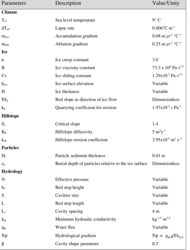
Parameters
Description
Value/Unity
Climate
Tsl Sea level temperature 9° C
dTair Lapse rate 0.006°C m-1
macc Accumulation gradient 0.08 m.yr-1 °C-1
mabl Ablation gradient 0.25 m.yr-1 °C-1
Ice
n Ice creep constant 3.0
B Ice viscosity constant 73.3 x 10⁶ Pa s1/3
Cs Ice sliding constant 1.29x10⁻² Pa s1/3
hice Ice surface elevation Variable
H Ice thickness Variable
∇𝑏𝑠 Bed slope in direction of ice flow Dimensionless
kq Quarrying coefficient for erosion 1.97x10⁻⁴ s Pa-3
Hillslope
Sc Critical slope 1.4
Kh Hillslope diffusivity 5 m2y-1
keh Hillslope erosion coefficient 3.95x10⁻⁵ m2 y-1
Particles
Hs Particle sediment thickness 0.01 m
zp Burial depth of particles relative to the ice surface Dimensionless Hydrology
N Effective pressure Variable
hs Bed step height Variable
S Cavities size Variable
L Bed step length Variable
Ls Cavity spacing 4 m
𝑘0 Minimum hydraulic conductivity kg-1/2 m3/2
qw Water flux Variable
∇𝜓 Hydrological gradient ∇𝜓 = 𝑞𝑤𝑔∇ℎ𝑖𝑐𝑒
β Cavity shape parameter 0.7
where B and n are the ice creep parameters. This hydrological model is similar that used in Ugelvig et al. (2016), and we therefore refer the reader to this study for more details.
In iSOSIA, the mass balance 𝑀 is linearly proportional to the mean annual air temperature Tair:
𝑀 = {−𝑚𝑎𝑐𝑐𝑇𝑎𝑖𝑟, 𝑖𝑓 𝑇𝑎𝑖𝑟 ≤ 0
−𝑚𝑎𝑏𝑙𝑇𝑎𝑖𝑟 , 𝑖𝑓 𝑇𝑎𝑖𝑟 > 0, (4)
where macc and mabl are the mass accumulation and the ablation gradients with respect to temperature, respectively. Tair is
5
assumed to decrease linearly with elevation ℎ with a lapse rate 𝑑𝑇𝑎𝑖𝑟 as
𝑇𝑎𝑖𝑟= 𝑇𝑠𝑙+ 𝑑𝑇𝑎𝑖𝑟. ℎ, (5)
where Tsl is the sea level temperature set constant at 9°C.
As mentioned in the introduction, the two main mechanisms of glacial erosion are abrasion and quarrying (Boulton, 1982; Hallet et al., 1996). As debris resulting from abrasion is mostly small in size (i.e. <50 μm, Hallet, 1979), we follow MacGregor 10
et al. (2009) and consider that this debris is instantaneously transported away from the glacial catchment by meltwater. However, quarrying acting on the lee side of bedrock steps by plucking can produce larger debris. Therefore, we consider in this study that sediments are only produced by quarrying. Quarrying is generally accounted for by a classical power-law basal sliding law, modified to account for some factors directly related to plucking (MacGregor et al. 2000; Kessler et al., 2008; MacGregor et al., 2009, Egholm et al., 2009; Herman et al., 2011). These factors include pre-existing fractures in the bedrock, 15
effective pressure, the regional bed slope in direction of ice flow, variation in meltwater drainage and the ice-bed contact area determined by the opening of cavities (Iverson, 2012; Cohen et al., 2006; Ugelvig et al., 2016; Anderson, 2014; Ugelvig et al., 2018). We follow Ugelvig et al. (2016) in modelling the quarrying rate Eq as
𝐸𝑞= 𝑘𝑞𝑁3𝑢𝑏(𝛻𝑏𝑠+ 𝑏𝑠0)2, (6)
where
k
qis a scaling coefficient for the effective pressure, N, that represents the effect of bedrock lithology and fractures, ∇𝑏𝑠 20is the bed slope in direction of sliding and bs0 is a term to allow for negative bed slopes. As we focus on glacier-induced
erosion, we ignore fluvial erosion and transport. However, we do consider hillslope erosion, which represents the supraglacial source of sediments. We assume that hillslope erosion, Eh, depends non-linearly on the bed gradient, as defined in (Andrew
and Bucknam, 1987) and (Roering et al., 1999):
𝐸ℎ = − 𝑘𝑒ℎ.𝛻𝑏 1−(|𝛻𝑏| 𝑆𝑐) 2, (𝟕) 25
where keh is an erodibility constant, and 𝑆𝑐 the critical slope.
2.2 Particle tracking and sampling
To investigate the detrital age distribution produced from a glaciated catchment, we need to track sediments from the source to their final site of deposition. Accordingly, we define “particles” as sediment trackers in our models. Sediments are produced as a result of local erosion. When sediment thickness exceeds a threshold Hs = 0.01 m, a particle is generated and can be
30
keeping a sufficient time resolution in the generation of particles (i.e. with an erosion rate of 1 mm yr-1 and H
s = 0.01 m a
particle is generated every 10 years in a cell). Depending on its position within the catchment, a particle is transported by different processes. Similar to Eq. (7), we assume that the flux, qph, of an unglaciated particle depends non-linearly on the bed
gradient (∇𝑏): 𝑞𝑝ℎ= − 𝐾ℎ. 𝛻𝑏 1 − (|𝛻𝑏|𝑆 𝑐 ) 2 , (8) 5
where 𝐾ℎ is the hillslope diffusion coefficient.
Glaciated particles can be incorporated into the ice either from the ice surface, for supraglacial debris, or from the ice-bed interface by basal quarrying. The horizontal velocity of each glaciated particle is computed as a function of their depth within the ice 𝑧𝑝, relatively to the ice surface. Because iSOSIA is a one-layer integrated model, the horizontal velocity depth-profile is computed following Glen’s flow law (Glen, 1952). We follow Rowan et al. (2015) in assuming that, due to the ice 10
viscosity, the horizontal ice velocity decays as a fourth-order polynomial of the ice thickness: 𝑢𝑝(𝑧𝑝) =
5 4[1 − 𝑧𝑝
4]𝑢̅ + 𝑢
𝑏, (9)
where 𝑢̅ = 𝑢̅𝑑+ 𝑢𝑏 is the average velocity of the ice, with ub the basal ice speed and 𝑢̅𝑑 the average velocity due to the internal deformation of the ice which is approximated as a tenth-order polynomial of the local ice thickness, the bed and ice surface gradients, as well as its curvature (Egholm et al., 2011). Velocity profiles for glaciated and unglaciated particles are 15
depicted in Fig. (S2).
The burial depth of particles (zp) within the ice is expressed relative to the ice surface (i.e. zp= 0 at the ice surface and 𝑧𝑝= 1 at its base, Fig. 1), and computed according to the mass balance:
Figure 1: Particle transport by ice. Particles originated from hillslopes enter to the glacier system from the surface (zp = 0), whereas particles
produced by the ice erosion are incorporated in the basal ice (zp = 1). The transport of glaciated particles follows the ice flow pattern from
𝜕𝑧𝑝
𝜕𝑡 =
𝑧𝑝𝑀̇𝑏−(1−𝑧𝑝)𝑀̇𝑠
𝐻 , (10)
where 𝜕𝑧𝑝
𝜕𝑡 is the change in burial depth of a particle through time, 𝑀̇𝑏and 𝑀̇𝑠 are the surface and basal melting at time t, respectively, and H is the ice thickness. Relative to the ice surface elevation, particles are moved downward according to the accumulation rate (in the accumulation zone 𝑀̇𝑠< 0 ), or upward with the lowering of the ice surface due to melting (in the ablation zone 𝑀̇𝑠> 0, Fig. 1).
5
In the experiments presented in the following sections, detrital particles are sampled throughout the frontal moraine, defined as the glacier tongue (Fig. 1 and Fig. 5d). As vertical mixing of sediment has been reported in some glacier fronts (Enkelmann et al., 2009; Grabowski et al., 2013; Enkelmann and Ehlers, 2015), we sample particles independently of their vertical position within the ice thickness to infer detrital age distributions.
2.3 Modelling the Tiedemann glacier
10
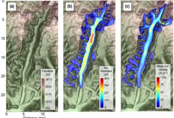
Our main goal is to investigate the influence of ice erosion and transport on the shape of detrital SPDFs. We present our modelling approach using the Tiedemann glacier (Coast Mountains, British Columbia, Canada, Fig. 2) as a case study. This
region has been previously studied using detrital and in situ thermochronology (Ehlers et al., 2015; Enkelmann and Ehlers, 2015). Moreover, the Tiedemann glacier has simple morphologic characteristics with a linear main glacial valley and small-extent tributary glaciers. Results of the simulations, mimicking the Tiedemann glacier, performed with iSOSIA are tested 15
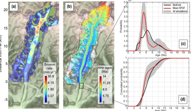
Figure 2: Satellite view of the Tiedemann glacier, British Columbia, Canada. The red contour represents the catchment area. The inset
shows the regional location, in the Coast Mountain range, Canada. Note the dominantly linear pattern of sediments transport (image from ©Google Earth, Maxar Technologies; inset map with data from Jarvis et al., 2008).
against the results of the ITMIX experiments (Farinotti et al., 2016; Farinotti et al., 2019) that predicts thickness of many glaciers around the world. The results of these calibration tests are shown in supplementary Fig. (S3). The reference iSOSIA Tiedemann glacier model is presented in Fig. (3). To produce synthetic detrital age distributions resulting from this reference model, we consider the glacier to be in steady-state and impose a constant topography (i.e. erosion produces particles but no topographic changes). The elevation of the Tiedemann glacier catchment ranges from 363 to 3920 m, for a total local relief of 5
3557 m. The resulting maximum ice thickness is 454 m with a mean ice velocity of 13.2 m yr-1, and a range of 0 to 109.2 m
yr-1, which are characteristics of Alpine glaciers (Benn and Evans, 2013). The mean velocity of the ice appears to be mainly
controlled by the basal sliding speed, which in turn is influenced by the shear stress on the bed and the distribution of open-cavities (Fig. S4). This results in two main part of relatively high velocities (~60 m yr-1) located at ~7 km and ~14 km in the
glacier latitudinal coordinates (Fig. 3c). 10
2.4 Synthetic ages and production of probability age distributions
To produce detrital SPDFs we need to specify the bedrock age distributions. Here, we predict ages for two thermochronological systems: the apatite (U-Th)/He (AHe) and apatite fission track (AFT). For the two systems, we consider the age-elevation relationship inferred from the bedrock data presented by Ehlers et al. (2015) for the Tiedemann glacier area (Fig. 4a). We use these as the basis of the bedrock age distribution in the catchment assuming that true AHe and AFT ages in the bedrock at a 15
Figure 3: Characteristics of the Tiedemann glacier model. (a) The underlying topography, (b) the ice thickness, and (c) the mean ice velocity.
given elevation are given by the age-elevation relationship. In practice, thermochronological analysis on a single-grain is presented as an age and its associated uncertainty. Thus, the measured age can be considered as a noisy sample of the true age. To produce a SPDF, we simulate this process for the detrital grain, and assume these are not modified during transport and deposition.
In Ehlers et al. (2015), AHe bedrock ages and therefore detrital data appear to have relatively high uncertainties (~21%). 5
However, we stress here that one of our goals is to assess the effect of age uncertainty on the interpretation of SPDF, and not to reproduce the SPDFs presented in Enkelman and Ehlers (2015). For this reason, we adopt uncertainties of 10% for the synthetic AHe ages sampled from the age-elevation profile. This is similar to the reproducibility in aliquots of single grain ages (e.g. ~6% Farley and Stocki, 2002).
The AFT data from Enkelmann and Ehlers (2015) show >30 % relative uncertainties. We generate synthetic AFT ages 10
following an approach similar to Gallagher and Parra (2020). We use the external detector method (EDM) age equation (e.g. Hurford and Green, 1983) to calculate the ratio of the spontaneous and the induced track density (𝜌𝑠/𝜌𝑖) corresponding to a given AFT age in the age-elevation profile. To allow for the effect of variable high uncertainties, we simulate the range of relative error of the Enkelmann and Ehlers (2015) study. To do this, we randomly sample values of Ns + Ni (i.e. the sum of the
number of spontaneous and induced tracks) from the data of Enkelmann and Ehlers (2015). We then use a binomial distribution 15
with parameter 𝜃 = 𝜌𝑠/𝜌𝑖
1+ 𝜌𝑠/𝜌𝑖 to sample Ns values, corresponding to the number of spontaneous tracks, given the sampled value
of Ns + Ni (see Gallagher, 1995; Galbraith, 2005). With the randomly sampled value of Ns, conditional on the sampled value
of Ns + Ni, we easily obtain a value for Ni. We can estimate a “noisy” AFT age and relative error from the sampled Ns and Ni
values by using the EDM equation. For both the AHe and AFT systems, we attribute for each particle a single age and uncertainty in accordance with its source location elevation.
20
The probability age distributions are then produced by using Gaussian kernel density estimate (Brandon, 1996; Ruhl and Hodges, 2005) with the mean and standard deviation equal to the age and error for both the AHe and AFT ages, following
𝑆𝑃𝐷𝐹𝑘 = 1 𝑁𝑝 1 𝛼𝜎𝑡√2𝜋 𝑒𝑥𝑝 [−1 2( 𝑡 − 𝑡𝑘 𝛼𝜎𝑡𝑘 ) 2 ] , (11)
where Np is the total number of sampled particles (i.e. ages), t is the range of ages in which we compute the SPDF, tk the age
of a particle considered, 𝜎𝑡the associated age uncertainty, and α = 0.6 is a scaling factor that handles the resolution and the 25
precision of age components in a SPDF (Brandon, 1996). To compare age distributions, we also define a cumulative synoptic probability density function, which is simply the cumulated sum of the SPDF:
𝐶𝑆𝑃𝐷𝐹 = ∑ 𝑆𝑃𝐷𝐹𝑗 𝑁𝑝
𝑗=0
(12)
Given the relatively high number of particles within the frontal moraine (i.e. > 106) and to mimic real detrital sampling, all the
detrital SPDFs presented in the following sections are produced by randomly sampling 105 particles from the total. This is 30
population (Vermeesch, 2004). We repeat this sampling process 10 thousand times, storing the resulting SPDFs. From all of these detrital SPDFs, we compute the mean detrital SPDF and present the range of inferred detrital distributions.
3 Results
3.1 Ideal detrital age distributions
5
The ideal detrital age distributions for the two thermochronological system, AHe and AFT, are presented in Fig. (4c-d). These are ideal in the sense that they represent the bedrock age distribution if we sample the total catchment uniformly, with noise added to the true ages sampled from the age elevation profile. In the subsequent text, we refer to these ideal detrital age distributions as the bedrock distributions. The bedrock AHe SPDF shows a major peak at ~6.3 Ma with two youngest smaller peaks at ~3.3 and ~4.3 Ma, and an older one ~11 Ma. The form of this SPDF mimics the hypsometric curve (black curve, 10
Figure 4: Age-elevation relationship for the two thermochronological systems AHe and AFT (a). Black and white circles represent the AHe
and AFT ages from (Ehlers et al., 2015). Solid black lines are the best fit solution for the data. Shaded area for the AHe age-elevation show the 10% uncertainty considered for AHe ages. The catchment hypsometry frequency as well as glaciers and hillslope hypsometry frequencies are presented in (b), and bedrock AHe and Aft distributions are in (c) and (d), respectively.
Fig. 4b) which is expected with a uniform production of sediments and a linear age-elevation relationship. The AFT SPDF shows a single major peak at ~15 Ma and the form does not mimic the hypsometric curve. This reflects partly the form of the age-elevation relationship, in which the ages below 2000 m (Fig. 4a) are similar, limiting the ability to resolve a unique relationship of age and elevation. We also note that, due to the high uncertainty, the probability to have an AFT age equal to zero is non-null.
5
3.2 Transport of detrital particles
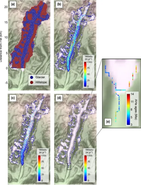
We investigate the kinematics of particles within our reference model for the Tiedemann glacier at the equilibrium state. One particle is produced in each cell of the model at a specific time (Fig. 5a) and transported away, potentially to the glacier front (i.e. the frontal moraine) where they would deposit. In this case, assuming we have reached steady state in terms of transport, differences between the final detrital and the bedrock SPDFs can only be related to the process of particle transport. Figures 10
5b-d show the evolution of particle locations at 500, 1000 and 8500 years after the production of particles. Obviously, the pattern of particle transport is consistent with the ice velocity field (Fig. 3c).
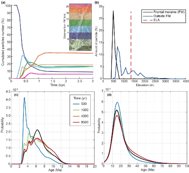
Figure 6 summaries the evolving contribution of particles from different locations to the detrital age distribution within the frontal moraine. First characteristic we point out is the minimum time, ~500 years, required for a particle originated from elevated parts of the catchment (i.e. far from the glacier front) to reach the frontal moraine (Fig. 6a, pink curve). Furthermore, 15
the proportions of particle sources in the frontal moraine becomes nearly constant after ~1500-2000 years (Fig. 6a). After 8500 years, some particles are still close to their sources (Fig. 5d). We find that only 44% of the initial particles have reached the front of the glacier and the frontal moraine (Fig. 6b, black curve, and Fig. S5a). The other 56% is trapped upstream, with a large part of them resting in a lateral moraine (Fig. 5d and 6b, blue curve) or on the side of small tributary glaciers having very slow velocities (i.e. < 1 m yr-1, Fig. 3c). These low velocities seem to result from a morphodynamic feedback where the
20
slope of tributary glaciers that carry the remaining particles is close to zero in the direction of sliding (Fig. S5b). This could, in turn, be related to the location of the ELA (Fig. 6b). As the number of particles within the frontal moraine does not increase significantly after 2000 years of simulation (i.e. reaching around 37% of the total number of initial particles, see Fig. S5a), we consider the steady-state of detrital SPDF to be reached at this time.
Figure 5e shows the spatial distribution of AHe ages within the frontal moraine after 8500 years, while Fig. (6c) shows the 25
transient evolution of the mean detrital probability AHe age distribution (SPDFs) in the frontal moraine and also the bedrock SPDF. For the detrital SPDFs, we observe a relative decrease of young ages (blue curves) with time during the transient phase, reflecting the progressive arrival of older ages coming from upstream and elevated parts of the catchment (see Fig. 4a and Fig. S6 for spatial bedrock age distributions). The form of detrital SPDFs reaches a steady-state around 4000 years of simulation (red and orange curves).
30
Focusing on the steady-state form of the detrital AHe SPDF (i.e. red curve), we can note differences with bedrock SPDFs (i.e. black curves). Indeed, the ~6.3 Ma age peak has a lower relative proportion than in the bedrock SPDF. We also observe a larger proportion of ages between 8 and 12 Ma in the detrital SPDF than in the bedrock SPDF. The two youngest age peaks,
at ~3.3 and ~4.3 Ma, are however well represented in the detrital SPDF. This suggests that the ice transport and deposit mid-ages, around 6 Ma (i.e. ~1500-2000 m), higher in the catchment.
For the AFT system (Fig. 6d), the peak age at ~16 Ma is similar for the detrital and bedrock distributions, but the magnitude of the final detrital age distribution peak is lower than the corresponding peak for bedrock. The relative contribution of old ages (> 25 Ma) is a little higher in the detrital SPDF, but for ages younger than 10 Ma, the distributions are similar. The 5
Figure 5: Example of particle transport. Particles have been uniformly produced across the catchment and transported. (a) Sources of
particles, (b) particles velocity at time = 500 yr, (c) at time = 1000 yr, and (d) at time = 8500 yr. AHe ages in the frontal moraine (FM) are shown in (e) and see inset in (d).
differences suggest that ice transport, and deposit sediments mostly originated from, 1000-2000 m in this case. We note that, the transient detrital SPDF at 1000 years best matches the bedrock curve.
3.3 Detrital signature under uniform catchment erosion
In this section, we consider a model with uniform erosion set at 1 mm yr-1, particles are then produced continuously (i.e. every
10 years) in each grid cell (Fig. 7a). In contrast to the previous simulation, which was run over 8500 years, these models were 5
terminated after 2000 years of simulation as the detrital SPDF in the frontal moraine is close to equilibrium (Fig. 4c).
Figure 6: (a) Cumulative contribution of source locations for particles in the frontal moraine, (b) their distribution with elevation after 8500
years of transport. (c) and (d) show the transient evolution of the detrital thermochronological age distribution in the frontal moraine for AHe and AFT systems respectively. Black curves represent the bedrock (ideal detrital) age distributions of each of the two systems.
This choice is also motivated by computational efficiency reasons as the number of tracked particles in the model increases rapidly with increasing run time. Our aim is to estimate the form of the detrital SPDF at the glacier margin by sampling the frontal moraine, and to compare it with what is expected for the case of uniform erosion. Indeed, we expect that the detrital distribution will mimic the hypsometric curve (i.e. the bedrock SPDF). Here we will focus our analysis on the AHe system for clarity. The detrital SPDFs of the AFT system can be found in the supplementary material (Fig. S7). Figure 7a shows the 5
spatial distribution of contributions from glacial and hillslope erosion processes, while the spatial distribution of detrital AHe ages after 2000 years of simulation is shown in Fig. (7b). The older ages are produced high in elevation, mainly by hillslope processes with local contribution from glacial erosion, whereas younger ages are produced by both hillslope and glacial erosion at lower elevation, according to the age-elevation relationship (Fig. 4a and Fig. S6a).
The detrital SPDFs resulting from the 10,000 sampling processes over the frontal moraine are summarised in Fig. (7g) where 10
the range of calculated SPDFs is represented by the grey shaded area. Here, we qualitatively describe the resulting SPDFs. We observe a large variability in detrital SPDFs resulting from sampling 105 particles in the frontal moraine with a maximum at ~3 Ma (Fig. 7g). The bedrock age distribution is always included in the range of inferred detrital SPDFs. The mean detrital SPDF (red curve) however, represents the “true” detrital signal we expect to obtain by considering all the particles in the sampling site. This mean detrital SPDF shows some differences to the bedrock SPDF (black curve). In particular, the main age 15
peak at ~6.3 Ma of the bedrock SPDF is not obviously represented in the mean detrital
SPDF similar to the previous model (Sect. 3.2), while the youngest age peaks at ~3.3 and ~4.3 Ma are over-represented. The proportion of old ages (> 8 Ma) is similar to the bedrock SPDF. We therefore have a clear under-representation of ages ranging from ~5 to ~8 Ma. Looking at the cumulative distributions of age probability (CSPDF), we see minor differences between the detrital CSPDF and the bedrock CSPDF, with the most obvious differences between 3 and 6 Ma.
20
The results for the AFT ages (see Fig. S7a-b and S7g-h) show a similar tendency in under-represented mid-age peak although less pronounced, with a maximum difference between the detrital and bedrock SPDFs at ~12.3 Ma and a smaller one at ~24.9 Ma. The AFT bedrock and detrital cumulated age distributions show a maximal difference at ~19.2 Ma, but overall are similar.
3.4 Detrital signature of glacier and hillslope sources
We now assess the respective influence of the two main sources of eroded particles, the glacier and ice-free hillslopes, on the 25
detrital SPDF. We first consider the ice-free hillslope source (Fig. 7c). Particles are produced by the mean erosion rate set at 1 mm yr-1, as in the case of uniform erosion, but only particles originating from ice-free areas are generated. The spatial AHe
age distribution after 2000 years of simulation displays ages ranging from 3.1 to 13.8 Ma (Fig. 7d) spanning ~96 % of the total age range (i.e. from 2.7 to 13.8 Ma). Thus, we compute a new bedrock SPDF according to the distribution of the sediment hillslope sources (black curve, Fig. 7i-j) that follow the hillslope hypsometry distribution (Fig. 4b). The maximum age range 30
Figure 7: (a) Source of particles for the three models experiments: uniform sources of particles, (c) hillslope source of particles, and (e)
glacier sources of particles, with Er being the erosion rate. Their respective spatial AHe ages distributions after 2000 yr of particle transport are shown in b-d-f. Density plots and their cumulative distributions are shown in g-h, i-j, and k-l respectively. The black squares show the frontal moraine (FM) position.
of inferred detrital SPDFs is in this case lower than the previous (Fig. 7i). The mean detrital SPDF shows a plateau-like signal from ~5 to ~9.5 Ma and differ from the hillslope bedrock SPDF, suggesting alone, uniform erosion for elevation from ~1400 to ~2500 m. However, a comparison with the bedrock SPDF indicates that storage of sediment occurs for such elevations. Moreover, the detrital SPDF is shifted toward old ages (> 8 Ma) and excludes ages lower than 3.5 Ma as the hillslope sources do not reach elevations showing such young ages. Thus, the mean detrital shows a maximum difference with the hillslope 5
bedrock CSPDF around 8 Ma (thick black curve, Fig. 7j). Therefore, constraining the hillslope sources for the bedrock SPDF allows to better identify the storage locations of sediments compare to the catchment bedrock SPDF (dashed curve, Fig. 7i-j). The mean AFT SPDF (Fig. S7i) shows a similar tendency in over-representing old ages (> 25 Ma) and under-representing mid-ages (~16 Ma) compared to the bedrock SPDF. However, the AFT SPDF differ from the AHe SPDF in that the bedrock AFT SPDF is always contained in the range defined by the shaded area and does not show a plateau-like form. Indeed, two 10
age peak components occur at ~16 Ma and at ~40 Ma. However, the detrital cumulated distribution (Fig. S7j) is shifted toward old ages with a maximum difference at 24.5 Ma. This difference is due to a different age-elevation relationship with lower spatial age resolution. Overall, the hillslope SPDFs reveal that the relevant source region ages tend to have older ages for both AHe and AFT.
We now consider the glacier source (Fig. 7e), which we define to be all the ice-covered areas. The detrital AHe ages range 15
from 2.7 to 12.1 Ma, spanning the first ~85% of the total age range of the catchment. The maximum age reflects the maximum elevation reached by the ice (i.e. ~3420 m). As previously, we compute a new bedrock SPDF according to the glacier source distribution (black curve, Fig. 7k) that is also in accordance with the glacial hypsometric curve (Fig. 4b). The detrital SPDFs shows a maximum range of inferred SPDFs at ~3.3 Ma (grey shaded area, Fig. 7k). Compared to the glacier bedrock SPDF, the mean detrital SPDF of the glacier source over-represents young ages (< 4 Ma), in contrast to the hillslope source as we 20
might expect. Next, we observe a relative under-representation of ages at ~6.3 Ma and for ages older than 8 Ma, consistent with a storage of sediment at mid-elevation. This is reflected in the cumulative detrital distribution (Fig. 7l), which is shifted towards younger ages and does not intersect the glacier bedrock cumulative distribution. The maximum difference between the two cumulative distributions is at 4.6 Ma.
The AFT distributions (Fig. S7k-l) show the same tendency in over-representing young ages (age peak at ~15.7 Ma) compared 25
to the glacier bedrock distribution and by under-representing old ages (>27.5 Ma). However, the differences are less pronounced. The cumulated distributions show a maximum difference at 28.1 Ma. We notice however a smaller difference between the detrital and the bedrock CSPDF for the AFT than for the AHe system. Overall, the differences are explained by the lack of older ages incoming from the glacier source.
3.5 Detrital signature using a landscape evolution model with non-uniform erosion
30
For the last numerical experiment, we look at the detrital age probability distribution within the frontal moraine resulting from the erosion laws presented in Sect. 2.1 with parameters listed in Table 1. This leads to a non-uniform model of erosion (Fig. 8a) with a mixture of hillslope- and glacier-origin sources for particles. The parameters of the erosion laws were calibrated by
a trial-error process to obtain a mean erosion rate over both source regions of 1 mm yr-1. Obviously, local deviations to this
mean value occur (e.g. 31 mm yr-1) as shown by the standard deviations for the mean erosion rates for the hillslope and glacier
sources of 1 ± 0.29 and 1 ± 2.9 mm yr-1 respectively, where the glacier erosion is more variable. Ice erosion pattern results
mostly from the distribution of effective pressure that controls the opening of cavities (Eq. 3 and Eq. 6) and therefore from the length on which the basal shear stress is applied (Eq. 1 and Fig. S1). Consequently, there are some ice-covered areas that do 5
not erode at all. The range of detrital ages for the glacier-origin particles spans 9 Ma from 2.7 to 11.7 Ma, whereas those for the hillslope-origin particles range from 3.5 to 13.8 Ma (Fig. 8b), reflecting both the sampling of the age-elevation relationship with higher elevation tend to be subjected to hillslope erosion, compared to glacier erosion that is mostly restricted to valley floors (Fig. 8a).
Looking at the detrital distributions (Fig. 8c), we observe large differences between the mean detrital and the catchment 10
bedrock SPDF. First, a single major age peak occurs at ~5 Ma, suggesting a predominant glacier source at ~1500 m. Second, an older age peak occurs at ~10 Ma, thus reflecting mostly the hillslope source and elevation ~2800 m (Fig. 8a). Very young ages (<4 Ma) are not represented as very low erosion rates (<0.07 mm yr-1) of glacier source occur at low elevations. The corresponding mean detrital CSPDF (Fig. 8d) shows a shift towards young ages compared to the bedrock CSPDF, the maximum difference between the two cumulated distribution being at 4.9 Ma. We also note that the bedrock CSPDF shows 15
Figure 8: Non-uniform erosion model experiment, with the (a) erosion rate, (b) the spatial AHe age distribution, (c) the density and (d)
clear departure from the range of possible detrital CSPDFs at ~6 Ma (grey shaded area, Fig. 8d), traducing a major glacier source contribution to the detrital SPDF of the frontal moraine.
The mean AFT detrital SPDF (Fig. S8c-d) shows no significant differences with the bedrock SPDF and bedrock CSPDF does not show departure from the range of possible detrital age distributions. This suggests a uniform erosion across the catchment, which is in contradiction with the conclusion inferred from the AHe system, that shows a major contribution of the glacier 5
source. This difference is due to the different age-elevation relationships and age uncertainties between the two thermochronometers, reducing in the case of the AFT system, the ability to track the source of particles. In this case, the AFT detrital distribution is not able to resolve the different contribution of the two sources (hillslope and glacier).
4 Discussion
4.1 Limitations of the particles transport model
10
It is important to note that the sediment particles in the model are transported passively and do not interact with the ice. For instance, the concentration of debris in the basal ice can influence the rheology of the ice and the friction of the bed, which both impact ice flow (e.g. Hallet, 1981; Iverson et al., 2003; Cohen et al., 2005). Surface debris-cover can also shield the ice from solar energy and in turn reduce the ablation rates and increase the local mass balance of the glacier (e.g. Östrem, 1959; Kayastha et al., 2000; Rowan et al., 2015). As iSOSIA does not perform a full 3D computation of ice deformation, the 15
horizontal velocity of particles is parametrized as a simple polynomial function (i.e. Eq. 9) of the average ice velocity (i.e. for englacial particles). Sediments can move vertically only by the accumulation of new ice or by melting, whereas natural particles can also move due to internal ice deformation, including thrusting and folding (Hambrey et al., 1999; Hambrey and Lawson, 2000). Surface debris may also fall in crevasses and therefore be incorporated in the basal ice (Hambrey et al., 1999). Lastly, sediment transport by rivers and sub-glacial drainage is neglected in the model.
20
4.2 Effect of sediment transport by the ice
Despite the limitations mentioned above, some first-order insights related to ice dynamics can be identified. Firstly, we characterize the time to reach an equilibrium in terms of the relative proportions of particles sources in the frontal moraine of around 1500 years. This time to reach equilibrium is similar to the timescale of the variability of glacier dynamics observed in valley glaciers (e.g. Nussbaumer et al., 2007; Osborn and Luckman, 1988). This suggests that a detrital age distribution 25
sampled from a glacial deposit like a frontal moraine may often reflect a transient case, with variable proportions of particle sources depending on the transport times (Fig. 6a). Thus, estimation of spatial erosion pattern can be biased based on the detrital SPDF (e.g. Ehlers et al., 2015). For instance, one may conclude that erosion is focused at low elevations (i.e. based on the young age peak in Fig. 6c). Secondly, zones of slow ice flow, such as in small tributary glaciers, may act as sediment traps as shown by particles remaining in elevated areas after 8500 years of simulation. These zones of slow ice occur mostly around 30
is more efficient around the ELA (e.g. Egholm et al., 2009; Brozović et al., 1997; Anderson et al., 2006; Steer et al., 2012), which leads to limited local relief and slope around the ELA and in turn to limited ice sliding velocity. This also highlights the role of morphodynamic feedbacks in controlling, here by a trapping effect, the detrital distribution of thermochronological ages. Therefore, only ~44% of the total initial number of particles have reached the frontal moraine after 8500 years of transport (i.e. the maximum time of our simulation). The remaining ~25 % of the particles are stored in the lateral moraine (Fig. 5d) and 5
the others ~31% are trapped at higher elevations, and therefore have residence times greater than 8500 years.
To illustrate in more detail the effect of low velocities on transport times, we compute the average transfer time as a function of source location for particles that reach the frontal moraine (Fig. 9). The results show that the time required for a particle to reach the frontal moraine is obviously not simply proportional to the distance between the moraine and the source location. Indeed, some particles formed near the frontal moraine may take more than 3000 years to reach the glacier front due to 10
velocities close to zero (Fig. 9a, red dots, and Fig. 9b, blue dots). In contrast, some particles formed far from the frontal moraine have transfer times less than 1000 years due to averaged-velocities greater than 15 m yr-1 (Fig. 9b). The proximity of the source
to ice streams with high velocities explains this pattern of transfer times (Fig. 3c). It is also illustrated in Figure 6a where we observe that particles originating 8 to 20 km from the frontal moraine arrive at the same time, and that the proportion of particles from 12-16 km evolves more rapidly than those from 8-12 km. It results that the average transfer times for particles 15
formed along hillslopes or glaciers are 1825.4 ± 1914.7 and 1084.9 ± 1014 yrs, respectively, but show high variability. This
Figure 9: Characteristics of particles transfer to the frontal moraine, (a) the time needed for each particle to reach the frontal moraine; (b)
difference is controlled 1) by the longer average distance of the hillslopes to the frontal moraine, 15.26 ± 7.19 km, compared to glaciers, 13.85 ± 6.15 km, and 2) by spatial variation in ice flow velocities and storage of sediment in small tributary glaciers. Overall, sediment transfer times are strongly influenced by the spatial distribution of small tributary glaciers, suggesting a control of the glacier size on the delivery of sediments to the main glacier transport system.
In the case of uniform erosion, combined with a linear relationship between thermochronological age and elevation (Fig. 4a), 5
we expect that the detrital thermochronological signal associated to each source mimics its associated hypsometric distribution. However, the resulting detrital SPDFs differ from that expected from the hypsometric distributions. The lack of the ages in the detrital SPDF corresponding to the peak observed ~1500-2000 m in the hypsometric curve, may be explained by (i) the storage of a major part of the sediments (i.e. 56%) outside of the sampling site, and (ii) by the patterns of transfer times for particles that have reached the frontal moraine (Fig. 9).
10
4.3 The role of detrital sources: glaciers or hillslopes
Each detrital source, i.e. hillslopes or glaciers, displays a different average hypsometry (Fig. 4b). Glaciers mostly represent valley floor while hillslopes mostly represent elevations greater than ~1800 m. We point out that hillslope sources contribute to older ages in the detrital SPDFs, as expected from the age-elevation profiles and the range of elevation of hillslope source (~700-4000 m). The glacial detrital SPDF (Fig. 7) reflects mainly the younger ages from the valley floor, and lack of older 15
ages as expected by the range of elevation occupied by glaciers (~530-3420 m). Moreover, depending on the erosion pattern, the proximity of the glacial source from the frontal moraine (<5 km) plays a role in the proportions of detrital age components, as the transfer times are lower (<300 years). The combination of the two source contributions is well illustrated in the case of uniform erosion through the catchment (Fig. 7), where the relative contribution of younger ages (glacier source) is reduced while the contribution of older ages better matches the bedrock distribution.
20
Characterizing the contribution of different sources and the nature of particle transport allows us to better understand the mean detrital SPDF of the frontal moraine resulting from non-uniform erosion (Fig. 8). Despite identical averaged erosion rates for the two sources (i.e. 1 mm yr-1 for hillslope and glacier respectively), glacial erosion shows a more heterogeneous pattern than
hillslope-erosion. The resulting young age peak component of the mean detrital SPDF (Fig. 8c, red curve) reflects a dominant glacial contribution to the frontal moraine. Indeed, local rates of erosion by quarrying, from 0 to ~31 mm yr-1, is observed to
25
be an order of magnitude greater than the maximum rate of hillslope erosion, from 0 to 2.3 mm yr-1 (Fig. 8a). Therefore, the
glacial process produces more particles which are ultimately transported to the frontal moraine. Furthermore, as glacial erosion is generally linked to the basal sliding speed (Eq. 6), we expect that glacial-origin sources of particles to be close to ice streams presenting high velocities, reducing in turn, the transfer time of such particles. Therefore, detrital SPDFs of glacial features like frontal moraine are likely to over-represent glacial sources of sediments compared to hillslopes sources. Next, a large part 30
of sediment particles produced on hillslopes originates from around 2800 m as illustrated by the older age peak component at ~10 Ma (Fig. 8c). This peak occurs because the elevated areas are connected to the main glacier and thus have transfer times,
~800 years, which are of the same order of those where the local erosion rate is highest (~31 mm yr-1, Fig. 8a). The spatial
distribution of hillslope erosion rates in Fig. 8a confirms this source elevation.
4.4 Implications for detrital sampling strategies
A sampling strategy equivalent to that considered in this study (i.e. randomly sampling the entire frontal moraine) has the potential to capture most of the bedrock age distribution. This is particularly true in the uniform erosion case where the mean 5
detrital SPDF approximates well the bedrock SPDF. However, given the advective nature of particle transport by ice, we now consider the effect of different sampling strategies. We perform an additional experiment, with uniform erosion, where sampling occurs in four different regions of the frontal moraine (Fig. 10). The process of sampling is the same as for previous models, i.e. we randomly collect 105 particles within each region, produce a SPDF and repeat this process 10,000 times to infer a mean detrital SPDF. The resulting mean AHe detrital SPDFs and CSPDFs are presented in Fig. 10. We first observe a 10
significant variability between the four detrital SPDFs. Sampling region one (Fig. 10) mostly represents young ages (<6 Ma) and therefore the glacier source. The hillslope source, with older ages (>6 Ma), is under-represented. Sampling regions two and three, located in the centre of the moraine, include an older age component (>6 Ma), which leads to a better fit with the mean detrital SPDF obtained by sampling the entire frontal moraine. We note that the detrital SPDF of region two seems to
Figure 10: Detrital AHe age distribution of the five sites seen in (b, black squares) from the experiment considering uniform source of
particles (a). The density plots and their cumulative distributions are shown in (c) and (d). The dashed black line is the mean detrital SPDF for the frontal moraine (FM).
better match the bedrock SPDF than the mean detrital SPDF. Finally, region four shows a bimodal age distribution with an over-representation of young (<4 Ma) and old ages (>7.5 Ma), and a gap in mid-ages (between 5 and 7 Ma) representing intermediate elevations (1500-2000 m). Focusing on the spatial distribution of detrital ages allows us to track the source of ages from the front of the glacier. We confirm that old ages (red dots in Fig. 10a-b) are mostly transported in the central part of the main glacier and deposited in the central part of the frontal moraine (regions two and three). An exception occurs with 5
region four due to deviation of ice streamlines (Fig. 10b). This deviation is also responsible for significant deposition of sediments in the lateral moraine. A high variability in detrital SPDFs is also observed at a smaller spatial scale, when considering a similar approach of Enkelmann and Ehlers (2015), where sediments are collected upstream of the frontal moraine along a transverse transect (see supplementary materials). Overall, local sampling within the frontal moraine or upstream along a transverse transect leads to a higher variability in the inferred detrital age distributions. Even if some regions may show better 10
agreement with the bedrock SPDF (region two), randomly sampling small patches of sediments through the moraine captures most of the age components on average and seems a better strategy.
4.5 The effect of age uncertainties and age-elevation profiles: comparing AHe and AFT
The detrital AFT SPDFs for the previous model considering sampling on four regions within the frontal moraine share similar pattern (Fig. S9). Region one over-represents young ages (<25 Ma) and under-represents old ages (>25 Ma). Region two is 15
like the bedrock SPDF, while region three and four tend to be biased toward older ages reflecting contributions from higher elevations. However, the variability between detrital AFT SPDF is much lower than for the detrital AHe SPDFs. Indeed, for all our models, we have seen that the behaviour of the mean detrital SPDFs from the AHe system differs from the AFT system. These differences occur for two main reasons. First, the age-elevation profiles differ. For the AFT profile, the youngest ages are not at the lowest elevation but occur at ~2000 m of elevation. The slope of the AFT age-elevation relationship is negative 20
(but almost vertical) for elevations lower than 2000 m. This low age-elevation gradient leads to a reduction in source identifiability, i.e. similar ages can come from a large range of elevations. Secondly, the high relative age uncertainties (i.e. >30%) in the AFT data smooths the SPDF and decreases the resolvability of age components in the age distribution. Consequently, these two characteristics can make the AFT system perhaps less useful for tracking erosion patterns (Enkelmann and Ehlers, 2015; Ehlers et al., 2015), as seen for the case of non-uniform erosion. However, in some cases the AFT distribution 25
can still capture first-order behaviour of sources if combined with bedrock age and age-elevation distributions, depending on the distribution of erosion across the catchment (Fig. S7i and Fig S9).
5 Conclusion
In this study, we have modelled the effect of erosion, ice transport and deposition on the distribution of thermochronological ages found in the frontal moraine of the Tiedemann glacier (British Columbia, Canada). Firstly, considering the kinematics of 30
is reached after 1500 yrs of ice transport. This result reflects the timescale of glacier dynamics and suggests that detrital SPDFs, in glaciated alpine catchments, are likely to reflect a transient case, especially for recent glacial deposits due for instance to glacier retreat. Secondly, the presence of small tributary glaciers, with very low velocities, may act as traps of sediment and delay particle transfer to the glacier front. These low velocities may result from a morphodynamic feedback between the location of the ELA and the bed slope in direction of sliding. Thirdly, the transfer times of sediments are not necessarily 5
correlated to the distance from the sampling site, as some sediments located in elevated areas may experience lower transfer times than sediments produced closer to the sampling site. This effect is also linked to the presence of small tributary glaciers with low velocities, and to the horizontal and vertical velocity distributions of the main glacier. Indeed, sources located at high elevations may deliver sediments directly to the centreline of the main glacier where the velocities are highest. Fourthly, lateral spread of ice flow lines may result in the deposition of lateral moraines that may store a significant amount of the sediments 10
produced upstream. Moreover, frontal moraines may have sediments that contain thermochronological signatures from only limited parts of the catchment, leading to a potential bias in the estimation of age distributions. To limit this issue, lateral moraines of the same age deposition as the frontal moraine can be also targeted for complementary sampling, therefore incorporating more age components.
Sediment transport by ice can introduces biases in the detrital age distributions, for instance by undersampling mid-altitudes 15
age components. This could lead to misinterpretation of regional erosion patterns. Therefore, an assessment of the spatial distribution of zones of low ice velocity, such as small tributary glaciers, and zones of intermediate storage of sediments may help to prevent such misinterpretation. Moreover, sampling strategies considering local sampling of sediments in the frontal moraine show variable detrital age distributions, that predominantly reflects the variability of local sources upstream. In principle, this may allow us to directly associate particle sinks, e.g. moraines, to their sources. In contrast, randomly sampling 20
through the frontal moraine potentially captures more age components, providing a more representative picture of the whole catchment. Therefore, we suggest applying such a sampling strategy when possible. However, we also emphasise the wide dispersion in detrital SPDFs that may result from sampling a limited amount of e.g. apatite grains (105 grains). Furthermore, we have systematically compared two thermochronological systems, AHe and AFT, with different but coherent age-elevation profiles and different relative age uncertainties. While the first plays a role in the ability to track sediment sources, the latter 25
decreases the precision of SPDFs if high. However, characterization of the spatial variability of source contribution between different sampling sites may still be possible depending on the distribution of erosion.
Overall, this study offers novel insights on the application of detrital thermochronology to glaciated catchments and on the role of long-term exhumation, modern erosion, and past sediment transport. Yet, our modelling approach neglects sediment transport by river and considers simple laws for ice motion and sediment entrainment. Future studies should focus on the role 30
of subglacial hydrology and ice plastic deformation on sediment transport and its associated detrital signal. Moreover, we have only considered one single alpine catchment and our results may not apply to larger ice systems, such as ice sheets. In particular, we have found that the detrital signal, recorded in the frontal moraine, reaches an equilibrium after 103 to 104 yrs, which is of
may inform on the impact of this variability on catchment erosion. Moraines of larger ice sheets, which are likely associated to a larger range of sediment transfer times, may prove more informative – and also more challenging - to constrain erosion rates integrated over longer timescales and several climatic cycles. In particular, sediments deposited along the margins of the Antarctica and Greenland ice sheets represent good candidates to explore erosion rates over a time scale of 105 to 106 yr.
Author contribution
5
Maxime Bernard developed the model code for the computation of thermochronological ages and SPDFs, designed the experiments, and prepared the manuscript with contributions from Philippe Steer and Kerry Gallagher. David L. Egholm provided the model iSOSIA with the associated knowledges to allow its use. He also contributed to the final version of the original draft.
Competing interest
10
The authors that they have no conflict of interest.
Acknowledgements
We thank Eva Enkelmann for having shared the AFT data from the Tiedemann glacier, which have been used to produce synthetics AFT ages. We also want to particularly thank Peter Van der Beek, Stephane Bonnet, Benjamin Guillaume, and Pierre Valla, for their advices and guidance that ultimately conducted to this study.
15
References
Anderson, R. S.: Evolution of lumpy glacial landscapes. Geology, 42(8), 679-682, 2014.
Avdeev, B., Niemi, N. A., and Clark, M. K.: Doing more with less: Bayesian estimation of erosion models with detrital thermochronometric data. Earth and Planetary Science Letters, 305(3-4), 385-395, 2011.
Alley, R. B., Cuffey, K. M., Evenson, E. B., Strasser, J. C., Lawson, D. E., and Larson, G. J.: How glaciers entrain and transport
20
basal sediment: physical constraints. Quaternary Science Reviews, 16(9), 1017-1038, 1997.
Beaumont, C., Fullsack, P., and Hamilton, J.: Erosional control of active compressional orogens. In Thrust tectonics (pp. 1-18). Springer, Dordrecht, 1992.
Benn, D., and Evans, D. J.: Glaciers and glaciation. Routledge, second edition, New York, USA, 2013.
Bernard, T., Steer, P., Gallagher, K., Szulc, A., Whitham, A., & Johnson, C.: Evidence for Eocene–Oligocene glaciation in the 25
Boulton G.S.: Processes and Patterns of Glacial Erosion. In: Coates D.R. (eds) Glacial Geomorphology. Springer, Dordrecht, 1982.
Brædstrup, C. F., Egholm, D. L., Ugelvig, S. V., and Pedersen, V. K.: Basal shear stress under alpine glaciers: insights from experiments using the iSOSIA and Elmer/Ice models. Earth Surface Dynamics, 4(1), 2016.
Brandon, M. T.: Probability density plot for fission-track grain-age samples. Radiation Measurements, 26(5), 663-676, 1996.
5
Brewer, I. D., Burbank, D. W., and Hodges, K. V.: Modelling detrital cooling-age populations: insights from two Himalayan catchments. Basin Research, 15(3), 305-320, 2003.
Brozović, N., Burbank, D. W., and Meigs, A. J.: Climatic limits on landscape development in the northwestern Himalaya. Science, 276(5312), 571-574, 1997.
Champagnac, J. D., Valla, P. G., and Herman, F.: Late-Cenozoic relief evolution under evolving climate: A
10
review. Tectonophysics, 614, 44-65, 2014.
Clarke, G. K.: A short history of scientific investigations on glaciers. Journal of Glaciology, 33(S1), 4-24, 1987.
Cohen, D., Iverson, N. R., Hooyer, T. S., Fischer, U. H., Jackson, M., and Moore, P. L.: Debris‐bed friction of hard‐bedded glaciers. Journal of Geophysical Research: Earth Surface, 110(F2), 2005.
Cohen, D., Hooyer, T. S., Iverson, N. R., Thomason, J. F., and Jackson, M.: Role of transient water pressure in quarrying: A
15
subglacial experiment using acoustic emissions. Journal of Geophysical Research: Earth Surface, 111(F3), 2006.
Egholm, D. L., Knudsen, M. F., Clark, C. D., and Lesemann, J. E.: Modeling the flow of glaciers in steep terrains: The integrated second‐order shallow ice approximation (iSOSIA). Journal of Geophysical Research: Earth Surface, 116(F2), 2011.
Egholm, D. L., Nielsen, S., Pedersen, V. K., and Lesemann, J.E: Glacial effects limiting mountain height, Nature, 460(7257), 884–887, 2009.
20
Egholm, D. L., Pedersen, V. K., Knudsen, M. F., and Larsen, N. K.: Coupling the flow of ice, water, and sediment in a glacial landscape evolution model. Geomorphology, 141, 47-66, 2012a.
Egholm, D. L., Pedersen, V. K., Knudsen, M. F., and Larsen, N. K.: On the importance of higher order ice dynamics for glacial landscape evolution. Geomorphology, 141, 67-80, 2012b.
Ehlers, T. A.: Crustal thermal processes and the interpretation of thermochronometer data. Reviews in Mineralogy and
25
Geochemistry, 58(1), 315-350, 2005.
Ehlers, T. A., Szameitat, A., Enkelmann, E., Yanites, B. J., and Woodsworth, G. J.: Identifying spatial variations in glacial catchment erosion with detrital thermochronology. Journal of Geophysical Research: Earth Surface, 120(6), 1023-1039, 2015. Enkelmann, E., and Ehlers, T. A.: Evaluation of detrital thermochronology for quantification of glacial catchment denudation and sediment mixing. Chemical Geology, 411, 299-309, 2015.
30
Enkelmann, E., Zeitler, P. K., Pavlis, T. L., Garver, J. I., and Ridgway, K. D.: Intense localized rock uplift and erosion in the St Elias orogen of Alaska. Nat. Geosci. 2 (5), 360–363, 2009.