Does probability of occurrence relate to population dynamics?

(1)

HAL Id: hal-01195082

https://hal.archives-ouvertes.fr/hal-01195082

Submitted on 27 May 2020

HAL is a multi-disciplinary open access archive for the deposit and dissemination of sci-entific research documents, whether they are pub-lished or not. The documents may come from teaching and research institutions in France or abroad, or from public or private research centers.

L’archive ouverte pluridisciplinaire HAL, est destinée au dépôt et à la diffusion de documents scientifiques de niveau recherche, publiés ou non, émanant des établissements d’enseignement et de recherche français ou étrangers, des laboratoires publics ou privés.

Does probability of occurrence relate to population

dynamics?

Wilfried Thuiller, Tamara Münkemüller, Katja H. Schiffers, Damien Georges,

Stefan Dullinger, Vincent M. Eckhart, Thomas C. Jr Edwards, Dominique

Gravel, Georges Kunstler, Cory Merow, et al.

To cite this version:

Wilfried Thuiller, Tamara Münkemüller, Katja H. Schiffers, Damien Georges, Stefan Dullinger, et al.. Does probability of occurrence relate to population dynamics?. Ecography, Wiley, 2014, 37 (12), pp.1155-1166. �10.1111/ecog.00836�. �hal-01195082�

(2)

non-equilibrium dynamics, and biotic interactions (Pulliam 2000). Competitive interactions could, for example, exclude a weak competitor from its optimal environmental condi-tions, while it might persist in more extreme environments that the dominant competitors cannot occupy (Loehle 1998, McGill et al. 2006). If population growth shows such negative density-dependence, the realized niche is the set of environmental conditions, x, where the intrinsic population

Ecography 37: 1155–1166, 2014

The niche concept is fundamental to our understanding of range dynamics. The niche is usually defined as the combi-nation of environmental conditions that allow a species to persist (Hutchinson 1957). One might expect that species are found if, and only if, the local environment is within their ‘demographic’ niche; i.e. where their intrinsic growth rate is positive. However, several ecological processes can lead to deviations from this expectation: source–sink dynamics,

Does probability of occurrence relate to population dynamics?

Wilfried Thuiller, Tamara Münkemüller, Katja H. Schiffers, Damien Georges, Stefan Dullinger, Vincent M. Eckhart, Thomas C. Edwards, Jr, Dominique Gravel, Georges Kunstler, Cory Merow, Kara Moore, Christian Piedallu, Steve Vissault, Niklaus E. Zimmermann, Damaris Zurell and Frank M. Schurr

W. Thuiller ([email protected]), T. Münkemüller, K. H. Schiffers and D. Georges, Laboratoire d’Ecologie Alpine (LECA), Univ. Grenoble Alpes, FR-38000 Grenoble, France. WT, TM, KHS and DG also at: CNRS, Laboratoire d’Ecologie Alpine (LECA), FR-38000 Grenoble, France. – S. Dullinger, Dept of Conservation Biology, Vegetation- and Landscape Ecology, Faculty Centre of Biodiversity, Rennweg 14, AT-1030 Vienna, Austria. – V. M. Eckhart, Dept of Biology, Grinnell College, Grinnell, IA, USA 50112. – T. C. Edwards,US Geological Survey, Utah Cooperative Fish and Wildlife Research Unit and Wildland Resources, Utah State Univ., Logan, UT 84322-5290, USA. – D. Gravel and S. Vissault, Dépt de Biologie, Chimie et Géographie, Univ. du Québec à Rimouski, 300 Allée des Ursulines, Québec G5L 3A1, Canada. – G. Kunstler, Irstea, UR Mountain Ecosystems, St-Martin-d’Hères, France. GK also at: Dept of Biological Sciences, Macquarie Univ., Sydney, NSW 2109, Australia. – C. Merow, Smithsonian Environmental Research Center, Edgewater, 21307-0028, MD, USA. – K. Moore, Center for Population Biology, Dept of Evolution and Ecology, Univ. of California, Davis, CA 95616, USA. – C. Piedallu, AgroParisTech, UMR1092, Laboratoire d’Étude des Ressources Forêt-Bois (LERFoB), ENGREF, Nancy Cedex, France. CP also at: INRA, UMR1092, Laboratoire d’Étude des Ressources Forêt-Bois (LERFoB), Centre INRA de Nancy, Champenoux, France. – N. E. Zimmermann and D. Zurell, Landscape Dynamics Unit, Swiss Federal Research Inst. WSL, Zuercherstrasse 111, CH-8903 Birmensdorf, Switzerland. DZ also at: Plant Ecology and Nature Conservation, Inst. for Biochemistry and Biology, Univ. of Potsdam, Maulbeerallee 2, DE-14469 Potsdam, Germany. – F. M. Schurr, Inst. des Sciences de l’Evolution de Montpellier, UMR-CNRS 5554, Univ. Montpellier II, 34095 Montpellier cedex 5, France. FMS also at: Inst. of Landscape and Plant Ecology, Univ. of Hohenheim, DE-70593 Stuttgart, Germany.

Hutchinson defined species’ realized niche as the set of environmental conditions in which populations can persist in the presence of competitors. In terms of demography, the realized niche corresponds to the environments where the intrinsic growth rate (r) of populations is positive. Observed species occurrences should reflect the realized niche when additional processes like dispersal and local extinction lags do not have overwhelming effects. Despite the foundational nature of these ideas, quantitative assessments of the relationship between range-wide demographic performance and occurrence probability have not been made. This assessment is needed both to improve our conceptual understanding of species’ niches and ranges and to develop reliable mechanistic models of species geographic distributions that incorporate demography and species interactions.

The objective of this study is to analyse how demographic parameters (intrinsic growth rate r and carrying capacity K ) and population density (N ) relate to occurrence probability (Pocc ). We hypothesized that these relationships vary with species’ competitive ability. Demographic parameters, density, and occurrence probability were estimated for 108 tree species from four temperate forest inventory surveys (Québec, western USA, France and Switzerland). We used published information of shade tolerance as indicators of light competition strategy, assuming that high tolerance denotes high competitive capacity in stable forest environments.

Interestingly, relationships between demographic parameters and occurrence probability did not vary substantially across degrees of shade tolerance and regions. Although they were influenced by the uncertainty in the estimation of the demographic parameters, we found that r was generally negatively correlated with Pocc, while N, and for most regions K, was generally positively correlated with Pocc. Thus, in temperate forest trees the regions of highest occurrence probability are those with high densities but slow intrinsic population growth rates. The uncertain relationships between demography and occurrence probability suggests caution when linking species distribution and demographic models.

(3)

growth rate (r(x)) is positive in the presence of competitors (Maguire 1973). Populations with a positive growth rate should also have a positive carrying capacity K.

The relationship between demographic parameters such as intrinsic growth rate (r(x)), carrying capacity (K ), abun-dance (N) and the probability of species occurrence (Pocc) has been studied theoretically (Holt 1997). The standard formu-lation of logistic growth holds that the equilibrium popula-tion size at a given locapopula-tion, K, will be independent to any variation of the intrinsic growth rate. The dynamics are given by the equation dN/dt  rN(1–N/K ), which takes the form

N*  K under equilibrium conditions. However, this

defini-tion suggests that density-independent factors affecting birth and death rates (and thus r) do not alter carrying capacity (Kuno 1991, Holt 1997, Gabriel et al. 2005). An ecologi-cally more intuitive alternative is to parameterize population models in terms of r and a per-capita competition coefficient

c (Kuno 1991). In these alternative parameterizations, K

increases with r (for the time-continuous logistic model and the time-discrete Ricker model K(x)  r/c), so that for con-stant c both r and K should increase with Pocc (Holt 1997). More complex relationships between K and Pocc can arise if competition intensity varies between populations. So far, there are very few empirical tests of these alternative predic-tions due to the unknown relapredic-tionships between Pocc and r,

K, and N (McGill 2012).

Species distribution models (SDMs, Guisan and Thuiller 2005) provide empirical estimates of Pocc by relating occur-rence (presence/absence) data to spatial variation in the environment. However, attempts to relate Pocc to measures of species’ local performance (e.g. variation in functional traits, Thuiller et al. 2010) or density N (VanDerWal et al. 2009, Canham and Thomas 2010) has provided mixed results. For instance, VanDerWal et al. (2009) showed that SDMs could predict maximum local N, but not mean N. The weak relationship between mean N and Pocc occurred because there was high variation in N at high Pocc, whereas consistently lower N was observed where occurrence Pocc was low. The environmental factors influencing Pocc may also differ from the ones affecting different aspects of demography such as N or r and K (Boulangeat et al. 2012). In addition, under meta-population dynamics, r will determine which environments are suitable for a species to establish a local population, but regional demographic processes will ultimately influence Pocc (Holt and Keitt 2000). Frequent patch extinctions relative to colonization events could eventually lead to regional extinc-tion, despite favourable environmental conditions.

When focusing on plant dynamics, and more particularly on trees, the relationship between demographic parameters and Pocc is dependent on several inter- and intra-specific factors as well as stochastic processes. For instance, high population growth may be observed at locations with low occurrence probability because the species has recently colonized a patch and is still far from equilibrium. Such population growth expectations will be influenced by spe-cies interactions and competitive ability. For trees, shade- tolerance is likely strongly related to r and K measured in the presence of competing species. Because shade intolerant trees typically establish first and reach their potential growth early during secondary succession, their occurrence probability should be highly positively correlated with r. Nevertheless,

those weaker (shade intolerant) competitors are more likely to be found away from their environmentally most suitable sites thereby potentially decoupling Pocc and K. In contrast, growth of shade tolerant species will often be reduced by increasing competitive interactions, leading to weaker cor-relations between Pocc and r. McGill (2012) recently showed for eastern North American trees that the environments in which species are most abundant are often not those in which individuals grow best. He interpreted this finding as an expression of ‘inclusive niche structuring’ (Loehle 1998) where all species share a similar optimal environment, but trade-offs between competitive ability and environmental tolerance cause weaker competitors with broader tolerance to be most abundant in suboptimal environments. However, it is not clear whether this analysis is indicative of large-scale variation in intrinsic population growth (r) because McGill (2012) did not correct for local density. Failure to include this correction precludes quantification of ‘intrinsic’ growth of individuals in the absence of conspecifics.

Despite these expectations, there is no published analysis of the relationships between demographic parameters and occurrence probability. Our main objectives in this study were thus: 1) to investigate how occurrence probability (Pocc), estimated by SDMs, is related to demographic param-eters (intrinsic population growth r, and K), and population density (N); and 2) to assess how these relationships vary with species’ competitive ability. To address these questions, we assembled forest–tree data sets from comprehensive inventories in Canada, France, USA and Switzerland. We used repeated census measurements to model changes in the density of tree populations as a function of density in the first census and topo-climatic variables. From these analyses, we obtained the intrinsic population growth rate (r) and the carrying capacity (K) of each population. We then estimated occurrence probability (Pocc) with species-specific SDMs for each of the study areas using the same topoclimatic variables. As a surrogate for competitive ability, we collected published information on all species’ shade tolerance, assuming that high tolerance denotes strong competitive ability. Finally, we investigated the relationships between demographic param-eters and occurrence probability, focusing either on all esti-mated data or only on the upper limit of these relationships (because stochasticity or disturbance might cause suboptimal performance in some populations), and analysed differences in relationships between shade-tolerance classes.

Material and methods

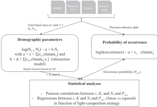
We compiled forest–tree datasets from four different areas in North America and Europe: Québec, western USA, France and Switzerland (Supplementary material Appendix 1, Fig. A1). For each dataset and for each species indepen-dently, we estimated the relationship between occurrence probability and demographic parameters (see Fig. 1 for a general workflow of the analysis). We used the same climatic variables in the SDMs to estimate occurrence probability and in the demographic models to estimate demographic parameters (Supplementary material Appendix 1, Table A1). We only retained plots not affected by harvesting between the censuses. Data for the distribution models consisted of

(4)

linear vs sigmoid

Figure 1. Workflow diagram depicting the analyses carried out in the paper. Nt and Nt  1 represent species-based total basal area at the first and second census, respectively. x correspond to the x climatic variables used in each study area.

recorded presence or absence at each sample plot for each study area.

In species with strongly size-structured populations (such as trees), the number of individuals is a poor descriptor of reproductive rates and the intensity of competition. Using only the number of individuals does not allow distinguishing a dense forest with a few large and reproductive trees from a sparsely vegetated site with a few small saplings. While the dynamics of size-structured populations could in principle be described with matrix models or integral projection mod-els, these models are rather data demanding and cannot be fully parameterized with the data available for this study. Instead, we took the simpler approach of expressing popula-tion dynamics as the dynamics of a species’ summed basal area (BA) in a plot. We chose BA because 1) it is used as a simple predictor for the intensity of competition in forest stands (Dale et al. 1985), and 2) it was found to be propor-tional to individual seed production for various tree species (Clark et al. 1999, Schurr et al. 2008). Hence, BA serves as a simple common currency that expresses the contribution of different size classes to both reproduction and competition in tree stands. Demographic data is described in more detail below.

Study areas

Québec

The forest inventory of the Québec Ministry of Natural Resources (MRNQ) is a network of permanent plots established in the 1970’s and re-measured approximately every decade (MRNQ 2013). The forest inventory cov-ers all public lands in Québec (80% of all forests), from temperate northern hardwoods to the boreal forests. By

including only plots with four measurements, which were not subject to major disturbance, we retained 11 062 plots in the analysis. Each sampling plot is circular and cov-ers 400 m2_{. Each tree with a diameter at breast height of}

9.1 cm or larger is tagged and re-measured in subsequent censuses. Recruits are added in each census. We report pop-ulation density as the summed basal area for each species (m2_ha1_{) and calculate population growth as the change}

in basal area between successive censuses. Because the interval between two censuses is not constant, we included the elapsed time between them to have an approximate measure of basal area increment per year. Overall, we had 31 species with more than 100 observations of basal area increment available for further analyses.

Western USA

The USDA Forest Service Inventory and Analysis (FIA) pro-gram maintains an extensive census of tree characteristics on public and private lands across USA (www.fia.fs.fed.us/). Data for 16 selected conifer species in western USA were extracted from this dataset. This subset was chosen based on sufficient presence–absence data information with high detection probability and repeated censuses. Information on the number and condition of trees is collected on plots approximately 0.4 ha in size. There was approximately one plot per 2400 ha, although spatial intensity of sample plots varies across USA. The FIA uses a panel rotation sample scheme for resampling of plots, with plots in the western study region resampled once every 10 years. Population densities and population growth were calculated from basal areas as described above. Data for analyses were restricted to western North America’s mid-latitude dry domain (after Bailey 1996) consisting of 1830 plots.

(5)

Nt Nt r Nt_{K t}    1 1 e

(

)

∆ (1)

where the expected density at time t  1 is a function of the density in the previous census N, r, K and the time interval between the censuses, ∆ t. Rearrangement and log-transformation of the Ricker model yields (Eq. 2):

log(Nt1/Nt)r t r t K N∆  ∆ /  t  a b Nt (2) which has the form of a linear regression of log-transformed density change against density in the previous census. This formulation assumes a relationship between r and K. We expanded this linear regression by including linear and quadratic effects of climatic variables. We considered two possible models: the first model contains only additive effects of climate and density so that

a z cx x

x n

 

∑

climate andbconst (3) The second model additionally describes climate effects on density dependence via an interaction between N and each climatic term a z cx x c x n x x x n

 

∑

climate and b d 

∑

(

climate e

)

(4) where x refers to a given climatic variable, Fig. 1).

In the model with interactions (Eq. 4), intraspecific competition intensity can vary with climate. In the model with only additive effects intraspecific competition inten-sity is constant. The best of the two alternative models for each dataset was selected using the small sample size cor-rected Akaike’s Information Criterion, AICc, (Akaike 1974, Burnham and Anderson 2002). This best model was then used to calculate the net reproductive rate r of each plot (the predicted change in density for Nt  0) and carrying capacity

K (the Nt at which change in density is 0).

In other words, r corresponds to the prediction of Eq. 3 or Eq. 4 for Nt  0. Because we took the log ratio of Nt  1 and Nt, it is actually the exponential of the prediction.

apredict Eq 3or Eq. 4 at( . ) Nt0 (5)

r__expa ₍₆₎

To estimate K, we made a prediction from Eq. 3 or Eq. 4 at

Nt  1 to extract the value of (a  b) and then subtract a to

isolate b.

bpredict(3)or(4)atNt 1 a (7)

K b

a (8)

Since some datasets had different time intervals between censuses, we standardized r by time-interval (∆t).

r t

 r

∆ (9)

For datasets with a hierarchical sampling block design (to account for multiple plots in western USA and for France

The French National Forest Inventory (http:// inventaire-forestier.ign.fr) comprises a network of temporary plots established on a sample of grid approxi-mately 1000  1000 m (plot randomly located in a square of 450 m around the centre of the cell) covering the French national territory between 2005 and 2011. The climate varies between Mediterranean, oceanic and continental, and is also strongly affected by elevation. For each measured tree, stem circumference, species, status (alive or died in the last 5 years), and radial growth over five years were recorded. The radial growth was determined from two short cores taken at breast height for 41 species. The basal area per species at the time of measurement was computed based on the cir-cumference of each living tree. We then computed the basal area five years earlier using the following information to reconstruct the stand: the five years radial growth of living trees, the trees that died between censuses, and the trees that recruited between censuses. We selected plots without har-vesting or planting between censuses leading to 22 592 plots. For more details on the data and the computation of basal area, see Supplementary material Appendix 1.

Switzerland

The Swiss National Forest Inventory (LFI) comprises a network of permanent plots covering Switzerland on a grid of approximately 1.4  1.4 km, with two concentric plots of 200 m2_{and 500 m}2_{respectively per grid cell (www.lfi.}

ch, Brändli 2010). The network contains ca 5974 plots that have been measured three times, while ca 1600 plots among these have been measured four times (in a panel rota-tion scheme since the third inventory period). The climate of the lowlands varies between sub-Mediterranean, oce-anic, continental and is also strongly affected by elevation. For each measured tree, stem circumference, species, status (alive or dead), and radial growth over ca 10 years (varies between 9 and 12 years) were recorded. Radial growth was determined from calliper re-measurements taken at breast height. The basal area per species at the time of measure-ment was computed based on the diameter of each living tree. We computed the basal area before and after the ca ten-year time step between re-measurement, and we corrected for the deviation from the ten-year interval as we did for the Québec data. Data were extracted for the 31 most common trees in Switzerland (Brändli 2010).

Estimation of demographic parameters

For each plot (considered as a population) and species, we calculated the proportional change in summed basal area (‘density’) between two successive censuses and related it to climatic conditions (Fig. 1). We initially checked that this proportional change was negatively related to species’ density at the first census as expected if competition causes negative density dependence of basal area change. This was done using Pearson’s correlations that indeed showed consis-tent and significantly negative relationships (Supplementary material Appendix 1, Fig. A2).

We fitted the Ricker model (Eq. 1) of population dynam-ics (Ricker 1954) to the data:

(6)

Analysing the relationship between density, demography and probability

We first analysed how demographic parameters are related to occurrence probability using Pearson’s correlation tests between r, K, N and occurrence probability. We corrected for multiple hypotheses testing using false discovery rate (i.e. the expected proportion of false discoveries amongst the rejected hypotheses).

Second, we built regression models to analyse the relationships between r, K, N and Pocc as a function of the study area and light-competition strategies. In addition, we also focused on the upper limit of the relationship between

r, K, N, and Pocc. We built quantile regressions by first classifying occurrence probability into 10 regular bins. Then, for each species and for each bin, we extracted the 75% quantile of r, K and N. This approach allowed us to have the same number of data points for each species and dataset. For both strategies, we tested for linear and sigmoid relationships between Pocc and the demographic param-eters (r, K and N) and retained the best model using AICc. This analysis was done for each species independently and the results were summarised by light-competition strategy. We recorded the form of the relationship selected (linear vs sigmoid), the slope (decreasing vs increasing) and the R2_of

the selected regression.

All calculations were carried out with R.3.0.1 using the stats and ggplot2 packages (Wickham 2009, R Development Core Team 2013).

Results

Demographic rates and occurrence probability

The estimation of r and K for each study area yielded demographic models with moderate goodness-of-fits and high variability between species (Supplementary material Appendix 1, Fig. A5). This suggests that changes in density were not easily modelled by the selected climate variables and intraspecific density-dependence (Supplementary mate-rial Appendix 1, Table A2). This limitation of modelled demographic parameters has to be taken into account when interpreting the relationships between demographic param-eters and occurrence probability. In addition, for some species, some plots had to be removed for the following analyses because positive density-dependence was observed, which violates the hypothesis underlying the Ricker model (Supplementary material Appendix 1, Table A2). In general, demographic models with low R2_{, especially for Québec and}

western USA, were associated with high uncertainty for both r and K (Supplementary material Appendix 1, Fig. A6). In comparison, SDMs had generally high predictive accuracy (Supplementary material Appendix 1, Fig. A4). r, K and

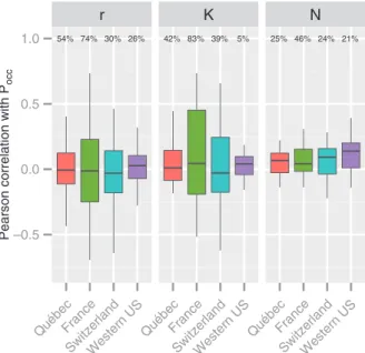
N were weakly to moderately correlated to Pocc across the four study areas (Fig. 2). The relationship between r or K and Pocc was variable within and between study areas, with both strongly positive and strongly negative correlations for France (Fig. 2). N was the parameter for which the percent-age of significant and positive correlations was the largest. multiple measurements in Québec and Switzerland),

we fitted the regressions as linear mixed-effects models including a random effect of block (Pinheiro and Bates 2000). Plots for which density-dependence was estimated to be positive (b  0) were omitted from further analy-ses since the Ricker model is not a plausible model for them (Supplementary material Appendix 1, Table A2 for the proportion of positive density-dependence for each species).

For each selected demographic model, we then extracted the goodness-of-fit (R2_{). For western USA, Québec and}

Switzerland, because mixed-effect models were used, we extracted the conditional R2_{, which corresponds to the}

goodness-of-fit estimated both fixed and random effects, respectively. R2_{values were extracted using the MuMIn}

(Bartoń 2013) package in R (R Development Core Team 2013). For France, goodness-of-fit was simply the R2_{of the}

linear models.

To assess whether the strength of the relationships between the demographic parameters and the probability of occurrence was influenced by uncertainty in the estima-tion of demographic parameters, we used non-parametric bootstrap resampling with 1000 bootstrap replicates. From 1000 bootstrap replicates, we computed the coefficient of variation of the bootstrap parameter estimates (standard deviation divided by the mean).

Species distribution models

We used generalised linear models (GLM) with linear and quadratic effects of climatic variables to estimate occur-rence probability for each species. Although GLMs are not necessarily the best performing models for SDMs (Elith et al. 2006), we chose them to avoid overfitting and to ensure comparability to the modelling procedure for demographic parameters. Because identification of a most parsimonious model was not the goal of the paper, we ran the GLMs on the full set of selected variables for each dataset (Supplementary material Appendix 1, Table A1). Models were evaluated by internal validation on the training dataset using the area under the curve (AUC, Swets 1988). In general, SDMs were relatively good at predicting current tree distribution in the four study areas. Only species with an AUC  0.7 were kept in the analyses (results for SDM and evaluations are in Supplementary material Appendix 1, Fig. A4, Table A2).

Light-competition strategy

We extracted information on species shade tolerance from (Niinemets and Valladares 2006) to test whether the relationship between occurrence probability and demographic performance was influenced by competi-tion for light (Shugart 1984, Bugmann 2001). We used a classification algorithm (kmeans) to group species into three groups: shade intolerant, moderately shade toler-ant and shade tolertoler-ant species (Supplementary material Appendix 1, Table A2, Fig. A3).

(7)

r K N 54% 74% 30% 26% 42% 83% 39% 5% 25% 46% 24% 21% –0.5 0.0 0.5 1.0 QuébecFrance SwitzerlandWestern US QuébecFrance SwitzerlandWestern US QuébecFrance SwitzerlandWestern US

Pearson correlation with

Pocc

Figure 2. Pearson correlation between probability of occurrence (Pocc) and r, K and N for each study area. The percentage of signifi-cant correlations (at p  0.05 controlled by false discovery rate) is indicated above each bar.

Influence of light-competition strategy

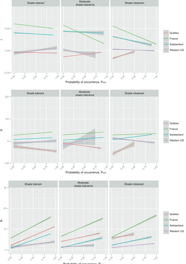
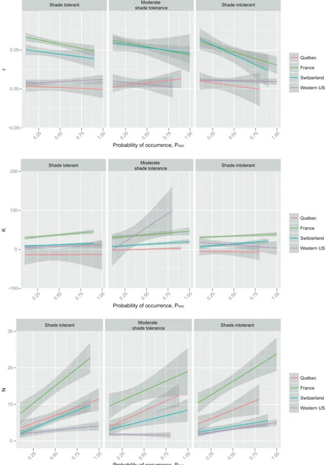
Multi-species regressions per study area and per light- competition strategy showed a general tendency for negative relationships between r and Pocc, for both standard and quan-tile regression approaches and for all light competition strat-egies (Fig. 3–4). The only exception was Québec for which positive relationships were generally detected. However, these relationships were based on negative r estimates. For both France and Switzerland, for which the relationships between r and Pocc were marked, the negative relationships tended to be steeper for shade intolerant species. K gener-ally showed a relatively weak but positive relationship to Pocc, the exception being Québec with negative relationships for shade and moderately shade tolerant species (Fig. 3). When using 75% quantile regressions, K–Pocc relationships were also weak but generally positive, except for western USA where it was slightly negative for shade intolerant species but strongly positive for moderately shade tolerant (Fig. 4). The relationship with density was more consistent and posi-tive for all regions and for both raw estimates (Fig. 3) and quantile estimates of demographic data (Fig. 4). Especially in France these positive relationships were strong.

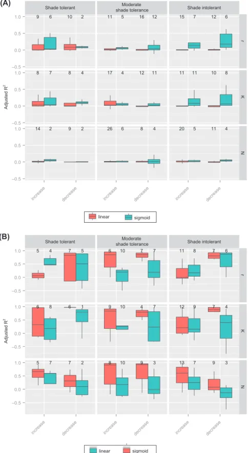
The goodness-of-fit of the regression models between each demographic parameter and occurrence probability was relatively low (Fig. 5A), and much higher when con-sidering quantile in comparison to standard regression approaches (Fig. 5B), although highly variable between species and within light-competition strategies (Fig. 5A–B). Interestingly, the adjusted R2_{reached higher values for shade}

intolerant species with sigmoid relationships between the demographic parameter and Pocc (Fig. 5A–B). When consid-ering quantile estimates of population properties, the number of significant results increased substantially, although a gen-eral trend was not easily distinguishable between light

com-petition strategies or the functional form of the relationship. This ambiguity was most pronounced for K. The slope of the

r–Pocc relationship tended to be negative for many species, especially for moderately shade tolerant species (Fig. 5B). However, when considering sigmoid relationships several species have positive relationships between r and Pocc. This was especially true for shade intolerant species (although the R2_{were relatively low). The slope of the K–Pocc relationship}

was more variable between light-competition strategies and no clear trend was distinguishable. The slope of the N–Pocc relationship was generally positive irrespective of the light-competition strategy.

The strengths of the above relationships were influenced by the precision of the demographic estimates (Supplementary material Appendix 1, Fig. A7). This was especially true for Québec and western USA for which low R2_{between r/K}

and Pocc were always found for species with highly uncer-tain parameter estimates (high coefficient of variation in the bootstrap estimates). For Québec, relationships between r/K and Pocc were significant for less than half species (14/24 for

r, 11/24 for K, and 7/24 for N, results not shown).

Discussion

Our analysis is the first to evaluate extensively the relation-ship between demographic performance and occurrence probability. Our study applied population demography approaches in a biogeographic context to test the common assumption of a positive relationship of r, K, and N with probability of occurrence. This assumption is at the corner-stone of the application of species distribution models in conservation (Araújo and Williams 2000). Our results reveal a wide range of relationships varying from moderately strong to no relationship of r, K and N to Pocc, although some vari-ability exists among regions and species. We also found these relationships to slightly vary with light competition strate-gies (shade tolerant vs shade intolerant), both in strength and shape but this was not as strong as expected. The major-ity of populations had positive r and K estimates (except populations in Québec for which parameter estimates were highly uncertain), which confirms the expectation that most populations occur within a species’ realized niche (Maguire 1973). Beyond this, different population properties revealed different relationships with occurrence probability, with a trend toward negative relationships for r when considering linear relationships but both positive and negative when considering sigmoid relationships, weak to moderate posi-tive trends for K, and posiposi-tive relationships for N whatever the shape of the relationship considered.

We stress two major findings:

1) For a number of species, we found no clear relation-ship of Pocc to r and K. This could have three explanations. First, the climatic variables used in our analyses may not adequately capture all processes that drive demography, such as disturbance or local microenvironments. Second, Pocc might not be very sensitive to variation in r and K within the range of conditions under which these species occur. While we confirmed the theoretical prediction that most popula-tions occur within their niche (r  0 and K  0), variation of Pocc within the niche might be affected by factors such

(8)

Shade tolerant _{shade tolerance}Moderate Shade intolerant

−0.05 0.00 0.05

0.00 0.25 0.50 0.75 1.00 0.00 0.25 0.50 0.75 1.00 0.00 0.25 0.50 0.75 1.00

Probability of occurrence, Pocc

r

Québec France Switzerland Western US

−100 0 100 200

0.00 0.25 0.50 0.75 1.00 0.00 0.25 0.50 0.75 1.00 0.00 0.25 0.50 0.75 1.00

K

0 10 20 30

0.00 0.25 0.50 0.75 1.00 0.00 0.25 0.50 0.75 1.00 0.00 0.25 0.50 0.75 1.00

N

Figure 3. Global relationship between occurrence probability (Pocc) and r, K and N with respect to species’ light-competition strategy and study area.

(9)

−0.05 0.00 0.05

0.25 0.50 0.75 1.00 0.25 0.50 0.75 1.00 0.25 0.50 0.75 1.00

r

−100 0 100 200

0.25 0.50 0.75 1.00 0.25 0.50 0.75 1.00 0.25 0.50 0.75 1.00

K

0 10 20 30

0.25 0.50 0.75 1.00 0.25 0.50 0.75 1.00 0.25 0.50 0.75 1.00

N

Figure 4. Global relationship between occurrence probability (Pocc) and 75% quantiles of and r, K and N with respect to species’ light-competition strategy and study area.

(10)

Shade tolerant _{shade tolerance}Moderate Shade intolerant 9 6 10 2 8 7 8 4 14 2 9 2 11 5 16 12 17 4 12 11 26 6 8 4 15 7 12 6 11 11 10 8 20 5 11 4 –0.5 0.0 0.5 1.0 –0.5 0.0 0.5 1.0 –0.5 0.0 0.5 1.0 r K N

increase decrease increase decrease increase decrease

Adjusted

R

2

linear sigmoid

Shade tolerant _{shade tolerance}Moderate Shade intolerant 5 4 7 5 6 8 6 1 5 7 7 2 6 10 7 7 9 10 4 7 8 10 9 3 11 8 7 6 12 9 7 4 13 7 9 3 –0.5 0.0 0.5 1.0 –0.5 0.0 0.5 1.0 –0.5 0.0 0.5 1.0 r K N

increase decrease increase decrease increase decrease

Adjusted R 2 linear sigmoid (B) (A)

Figure 5. R2_{values of regression models between and r, K and N, and P}

occ as a function of light-competition strategy. The slope (decreasing or increasing) of the regression is indicated. The number at the top of each bar corresponds to the number of species for which the model (linear or sigmoid) was selected by AIC. (A) boxplot corresponding to the analyses carried out with all raw data, (B) with 75% quantiles.

(11)

et al. (2012). Using a hierarchical and nested approach, they showed that biotic interactions were the primary drivers of variation in abundance along environmental gradients, whereas the presence and absence of plant species were bet-ter predicted by the abiotic environment and by dispersal (Boulangeat et al. 2012).

The main limitations of our analysis are both the complexity of estimating forest population dynamics and the substantial differences between study areas. Size struc-ture is extremely important in forest ecosystems and com-plicates the estimation of population dynamics (Easterling et al. 2000). To circumvent these complications, we fitted population models using summed basal area as a state vari-able that implicitly represents size structure in even aged stands. Additionally, to appropriately model the relationship between estimated demographic parameters and occurrence probability, a large number of data points is required to estimate the lower end of the relationship between demo-graphic rate and occurrence probability (negative or null

r for very low probability of occurrence). Such conditions

are unlikely to be found in the forest systems in our study after centuries of management. For instance, if we exclude Québec, estimated r almost never reached values close to 0. In reality, we may only capture positive growth rates where species have ‘viable’ populations and the positive or negative relationships only reflect differential effects of inter-specific competition and stochastic events.

Another limitation is the estimation of demographic parameters. We assumed that density-dependence and cli-mate influence demography and we used a simple population model (Ricker population model, Ricker 1954) to estimate

r and K. The resulting demographic models varied

consider-ably in their goodness-of-fit between species and study areas. SDMs, on the other hand, were of good quality across the study areas. The combination of relatively exact estimates of occurrence probability and relatively inaccurate estimates of demographic parameters likely contributed to the low number of significant relationships. This was mostly the case for Québec for which the quality of the demographic estimates is highly questionable and could explain the very low values (often negative) of r and K for those species. The bootstrap estimates for this region showed that there was a very high uncertainty for these parameters. The elevated variance in the parameter b might result in a bias estimate of

K because of Jensen’s inequality. If only b is varying, then it

should lead to a systematic underestimation of K, with the bias linearly proportion to the variance. Since a and b are covarying, the consequence of their joint variability on K is not straightforward to estimate (Gravel et al. 2011). The solu-tion to the problem would be evaluate the parameters using a Markov chain Monte Carlo method and to compute the posterior distribution of K. Running this scheme for all datasets and all species is however far beyond the scope of the paper. The results from Quebec are the most likely affected by this problem because of the low quality of the fit. In this paper we only use the Ricker model for practi-cal reasons since it has the convenient property that it can be fit with linear (mixed) models (which is not the case for e.g. the theta-logistic). Fitting alternative models would have required custom-coding of hierarchical non-linear models. We thus chose to stay with this simple demographic model, as the spatial arrangement of suitable habitat, competitive

interactions, and dispersal (Holt and Keitt 2000). Third, for a number of species our demographic estimates may be too uncertain. In other words, the models do not fully capture the true demography of the populations. This may explain why we found weak relationships for species from Québec and some species from western USA.

2) r and K show qualitatively different relationships to

Pocc. r tends to be negatively correlated with Pocc whereas K,

in contrast, was mostly found to be constant or increasing with Pocc, independently of shade tolerance. The relation-ship between r and K is determined by the intensity of intraspecific competition (parameter b in Eq. 3 and 4): the overall finding that r tended to decrease with Pocc whereas

K was constant or increased therefore implies that

intraspe-cific competition is less intense in environments with high occupancy. The effect of interspecific competition could also explain this pattern. However, interspecific competition should simultaneously lower both r and K. The opposite direction between r and Pocc, and, K and Pocc can thus only

explain our findings if there is a negative correlation between

Nt and the presence/abundance of other species. As

inter-specific competition goes up, the density of other species goes down. Remarkably, r and K were both often negative for species for Québec. Because we removed cases with posi-tive density-dependence, there is one way to have a negaposi-tive carrying capacity with our calibration of the Ricker model: a negative intrinsic rate of increase). While this situation is possible in nature (e.g. if a species is outside of its niche), it most likely arose because a poor fit of the model to the data (Supplementary material Appendix 1, Fig. A6 and Fig. 7). Another non-exclusive reason is the occurrence of natural disturbances. While these are unlikely to generate a negative growth rate or carrying capacity (it would require a majority of the plots being disturbed), it could nonetheless generate a significant amount of noise. This is particularly true for the boreal forest of Quebec, where a severe outbreak of the spruce budworm affected the fir and spruce stands during the 1980–1995 period. This massive and synchronized dis-turbance is a likely cause of the low fit to the model we find in this dataset. Logging might also interrupt the dynamics of the stand, but it should be minimal in this dataset since the plots are supposed to be protected.

These summary points corroborate, to some degree, the results from McGill (2012) who tested whether tree individu-als grow best where the species is found to be most abundant. McGill found a negative relationship between ontogenetic growth rate and abundance for trees in eastern North America across 15 species. He argued that this result is not compatible with MacArthur’s (1958) vision of an exclusive niche, in which species should be most common at the optimum of their envi-ronmental niche and should have distinct optima from one another. Yet, it is not clear whether the negative relationship between individual growth and abundance did not simply result from intraspecific density dependence.

The observed positive relationship between occurrence probability and N supports previous findings that occurrence probability can predict maximal abundance (VanDerWal et al. 2009). The fact that Pearson correlations and R2

were relatively low when considering the full distribution of density (Fig. 3–4) also corroborates findings by Boulangeat

(12)

workshops entitled ‘Advancing concepts and models of species range dynamics: understanding and disentangling processes across scales’. Funding was provided by the Danish Council for Indepen-dent Research – Natural Sciences (grant no. 10-085056). CM acknowledges funding from National Science Foundation (NSF) grant 1046328 and NSF grant 1137366. KM acknowledges fund-ing from NSF grant DEB-0919230. DZ acknowledges fundfund-ing by DFG grant WI 3576/1-1. The work of FMS was supported by German Research Foundation (DFG) grant SCHU 2259/5-1. GK was supported by a Marie Curie International Outgoing Fellowship within the 7th European Community Framework Program (Demo-traits project, no. 299340). We are thankful for access to forest inventory data of France, Quebec, western USA and Switzerland. Most of the computations presented in this paper were performed using the CIMENT infrastructure (https://ciment.ujf-grenoble. fr), which is supported by the Rhône-Alpes region (GRANT CPER07_13 CIRA: http://www.ci-ra.org) and France-Grille (www.france-grilles.fr). WT belongs to the LECA, part of Labex OSUG@2020 (ANR10 LABX56).

References

Akaike, H. 1974. A new look at statistical model identification. – IEEE Transactions on Automatic Control AU-19: 716–722. Anderson, B. J. et al. 2009. Dynamics of range margins for meta-populations under climate change. – Proc. R. Soc. B 276: 1415–1420.

Araújo, M. B. and Williams, P. 2000. Selecting areas for species persistence using occurrence data. – Biol. Conserv. 96: 331–345. Bailey, R. G. 1996. Ecosystem geography. – Springer Verlag. Bartoń, K. 2013. MuMIn: multi-model inference.

– http://R-Forge.R-project.org/projects/mumin/. Boulangeat, I. et al. 2012. Accounting for dispersal and biotic

interactions to disentangle the drivers of species distributions and their abundances. – Ecol. Lett. 15: 584–593.

Brändli, U.-B. 2010. Schweizerisches Landesforstinventar. Ergebnisse der dritten Erhebung 2004–2006. – Birmensdorf, Eidgenössische Forschungsanstalt für Wald, Schnee und Land-schaft WSL.

Bugmann, H. 2001. A review of forest gap models. – Clim. Change 51: 259–305.

Burnham, K. P. and Anderson, D. R. 2002. Model selection and multimodal inference: a practical information-theoretic approach. – Springer-Verlag.

Canham, C. D. and Thomas, R. Q. 2010. Frequency, not relative abundance, of temperate tree species varies along climate gradients in eastern North America. – Ecology 91: 3433–3440.

Clark, J. S. et al. 1999. Interpreting recruitment limitation in forests. – Am. J. Bot. 86: 1–16.

Dale, V. H. et al. 1985. A comparison of tree growth-models. – Ecol. Modell. 29: 145–169.

Dullinger, S. et al. 2012. Extinction debt of high-mountain plants under twenty-first-century climate change. – Nat. Clim. Change 2: 619–622.

Easterling, M. R. et al. 2000. Size-specific sensitivity: applying a new structured population model. – Ecology 81: 694–708. Elith, J. et al. 2006. Novel methods improve prediction of

species’ distributions from occurrence data. – Ecography 29: 129–151.

Fordham, D. A. et al. 2012. Plant extinction risk under climate change: are forecast range shifts alone a good indicator of species vulnerability to global warming? – Global Change Biol. 18: 1357–1371.

Franklin, J. 2010. Moving beyond static species distribution models in support of conservation biogeography. – Divers. Distrib. 16: 321–330.

which is easily tractable. Future studies with a focus on a specific site and thus more detailed data could explore a wider range of demographic models.

Understanding the relationship between demographic parameters and occurrence probability is critical for evaluat-ing the assumptions made by recent modellevaluat-ing approaches that aim to project species’ future distributions under climate change scenarios (Franklin 2010). Indeed, SDMs cannot directly model dispersal effects, local demography or inter-specific competition, which makes them unsuitable to simulate range dynamics. Reciprocally, projecting spatially explicit demographic models through time requires informa-tion on local demography over a broad range of environmen-tal conditions. In attempts to predict species range dynamics, SDM outputs have been used to scale spatially explicit meta-population models (Keith et al. 2008), stage-structured populations (Dullinger et al. 2012), or individual-based models (Zurell et al. 2012). These frameworks originate from the goals of projecting species’ distributions under changing environmental conditions and to account for the transient dynamics in these projections. Integrating demographic and occurrence data in a hierarchical statistical model is an emerging solution, yet still poses substantial conceptual and methodological challenges (Schurr et al. 2012). Our results caution against untested use of occurrence probabil-ity estimates from SDM to infer demographic performance, because the form and the strength of the relationship may strongly differ between species and area. For example, several modelling attempts have scaled maximum carrying capacity by occurrence probability (Anderson et al. 2009, Fordham et al. 2012). Here we showed that the positive relationships between K and probability of occurrence are relatively weak (even for the upper quantiles), and the form of the relation-ship seems species-specific. Hence, careful examination or validation of the relationship is a clear pre-requisite before using such scaling techniques in any biodiversity modelling approach.

Conclusion

We tested how variation in demographic quantities relates to variation in occurrence probability along environmen-tal gradients. These relationships varied greatly in nature because of the interacting effects of habitat suitability, inter-specific competition and intra-specific density- dependence. Our study is the first to test these relationships between performance and occurrence probability, and from our analyses we cannot conclude that a strong relationship exists. Rather, we find that the hypothesis holds for some species groups in some circumstances while it does not in other groups. In this respect, complementary research is needed on other taxa and regions to determine why dif-ferences in occurrence–demography relationships exist. This will help to better understand if and when occurrence is a suitable proxy for demography.

Acknowledgments – The research leading to this paper had received funding from the European Research Council under the European Community’s Seven Framework Programme FP7/2007-2013 grant agreement no. 281422 (TEEMBIO). This study arose from two

(13)

Niinemets, Ü. and Valladares, F. 2006. Tolerance to shade, drought, and waterlogging of temperate Northern Hemisphere trees and shrubs. – Ecol. Monogr. 76: 521–547.

Pinheiro, J. C. and Bates, D. M. 2000. Mixed-effects models in S and S-Plus. – Springer-Verlag.

Pulliam, H. R. 2000. On the relationship between niche and distribution. – Ecol. Lett. 3: 349–361.

R Development Core Team (ed.) 2013. R: a language and environ-ment for statistical computing. – R Foundation for Statistical Computing.

Ricker, W. E. 1954. Stock and recruitment. – J. Fish. Res. Board Canada 11: 559–623.

Schurr, F. M. et al. 2008. Plant fecundity and seed dispersal in spatially heterogeneous environments: models, mechanisms and estimation. – J. Ecol. 96: 628–641.

Schurr, F. M. et al. 2012. How to understand species’ niches and range dynamics: a demographic research agenda for biogeogra-phy. – J. Biogeogr. doi: 10.1111/j.1365-2699.2012.02737.x. Shugart, H. H. 1984. A theory of forest dynamics. The ecological

implications of forest succession models. – Springer-Verlag. Swets, K. A. 1988. Measuring the accuracy of diagnostic systems.

– Science 240: 1285–1293.

Thuiller, W. et al. 2010. Variation in habitat suitability does not always relate to variation in species’ plant functional traits. – Biol. Lett. 6: 120–123.

VanDerWal, J. et al. 2009. Abundance and the environmental niche: environmental suitability estimated from niche models predicts the upper limit of local abundance. – Am. Nat. 174: 282–291.

Wickham, H. 2009. ggplot2: elegant graphics for data analysis. – Springer.

Zurell, D. et al. 2012. Uncertainty in predictions of range dynamics: black grouse climbing the Swiss Alps. – Ecography 35: 590–603.

Gabriel, J. R. et al. 2005. Paradoxes in the logistic equation? – Ecol. Modell. 185: 147–151.

Gravel, D. et al. 2011. Species coexistence in a variable world. – Ecol. Lett. 14: 828–839.

Guisan, A. and Thuiller, W. 2005. Predicting species distribution: offering more than simple habitat models. – Ecol. Lett. 8: 993–1009.

Holt, R. D. 1997. On the relationship between range size and local abundance: back to basics. – Oikos 78: 183–190.

Holt, R. D. and Keitt, T. H. 2000. Alternative causes for range limits: a metapopulation approach. – Ecol. Lett. 3: 41–47. Hutchinson, G. E. 1957. Concluding remarks. – Cold Spring

Harbor Symp. Quant. Biol. 22: 145–159.

Keith, D. A. et al. 2008. Predicting extinction risks under climate change: coupling stochastic population models with dynamic bioclimatic habitat models. – Biol. Lett. 4: 560–563. Kuno, E. 1991. Some strange properties of the logistic equation

defined with r and K: inherent defects or artifacts? – Res. Pop. Ecol. 33: 33–39.

Loehle, C. 1998. Height growth rate tradeoffs determine northern and southern range limits for trees. – J. Biogeogr. 25: 735–742.

MacArthur, R. H. 1958. Population ecology of some warblers of northeastern coniferous forests. – Ecology 39: 599–619. Maguire, B. 1973. Niche response structure and analytical

poten-tials of its relationship to habitat. – Am. Nat. 107: 213–246. McGill, B. J. 2012. Trees are rarely most abundant where they grow

best. – J. Plant Ecol. 5: 46–51.

McGill, B. J. et al. 2006. Rebuilding community ecology from functional traits. – Trends Ecol. Evol. 21: 178–185.

MRNQ 2013. Ministère des Ressources Naturelles du Québec – Placettes-échantillons permanentes (2013). Direction des inventaires forestiers – Secteur des forêts, Ministère des Ressources Naturelles, p 231.

Supplementary material (Appendix ECOG-00836 at www.ecography.org/readers/appendix). Appendix 1.