Direct characterization of young giant exoplanets at high spectral resolution by coupling SPHERE and CRIRES+

HAL Id: hal-03147429

https://hal.archives-ouvertes.fr/hal-03147429

Submitted on 19 Feb 2021

HAL is a multi-disciplinary open access

archive for the deposit and dissemination of

sci-entific research documents, whether they are

pub-lished or not. The documents may come from

teaching and research institutions in France or

abroad, or from public or private research centers.

L’archive ouverte pluridisciplinaire HAL, est

destinée au dépôt et à la diffusion de documents

scientifiques de niveau recherche, publiés ou non,

émanant des établissements d’enseignement et de

recherche français ou étrangers, des laboratoires

publics ou privés.

Direct characterization of young giant exoplanets at high

spectral resolution by coupling SPHERE and CRIRES+

G. P. P. L. Otten, A. Vigan, E. Muslimov, M. N’diaye, E. Choquet, U.

Seemann, K. Dohlen, M. Houllé, P. Cristofari, M. W. Phillips, et al.

To cite this version:

G. P. P. L. Otten, A. Vigan, E. Muslimov, M. N’diaye, E. Choquet, et al.. Direct characterization of

young giant exoplanets at high spectral resolution by coupling SPHERE and CRIRES+. Astronomy

and Astrophysics - A&A, EDP Sciences, 2021, 646, pp.A150. �10.1051/0004-6361/202038517�.

�hal-03147429�

c

G. P. P. L. Otten et al. 2021

_Astrophysics

&

Direct characterization of young giant exoplanets at high spectral

resolution by coupling SPHERE and CRIRES+

G. P. P. L. Otten

, A. Vigan

, E. Muslimov

, M. N’Diaye

, E. Choquet

, U. Seemann

, K. Dohlen

, M. Houllé

,

P. Cristofari

, M. W. Phillips

, Y. Charles

, I. Baraffe

, J.-L. Beuzit

, A. Costille

, R. Dorn

, M. El Morsy

,

M. Kasper

, M. Lopez

, C. Mordasini

, R. Pourcelot

, A. Reiners

, and J.-F. Sauvage

1 _{Aix Marseille Univ, CNRS, CNES, LAM, Marseille, France}

e-mail: gilles.otten@lam.fr

2 _{Kazan National Research Technical University named after A.N. Tupolev KAI, 10 K. Marx, Kazan 420111 Russia} 3 _{Université Côte d’Azur, Observatoire de la Côte d’Azur, CNRS, Laboratoire Lagrange, Bd de l’Observatoire, CS 34229,}

063404 Nice Cedex 4, France

4 _{Institute for Astrophysics, Georg-August University, Friedrich-Hund-Platz 1, 37077 Göttingen, Germany} 5 _{School of Physics and Astronomy, University of Exeter, Exeter EX4 4QL, UK}

6 _{European Southern Observatory (ESO), Karl-Schwarzschild-Str. 2, 85748 Garching, Germany} 7 _{Physikalisches Institut, University of Bern, Sidlerstrasse 5, 3012 Bern, Switzerland}

Received 28 May 2020/ Accepted 27 August 2020

ABSTRACT

Studies of atmospheres of directly imaged extrasolar planets with high-resolution spectrographs have shown that their characterization is predominantly limited by noise on the stellar halo at the location of the studied exoplanet. An instrumental combination of high-contrast imaging and high spectral resolution that suppresses this noise and resolves the spectral lines can therefore yield higher quality spectra. We study the performance of the proposed HiRISE fiber coupling between the direct imager SPHERE and the spectrograph CRIRES+ at the Very Large Telescope for spectral characterization of directly imaged planets. Using end-to-end simulations of HiRISE we determine the signal-to-noise ratio (S/N) of the detection of molecular species for known extrasolar planets in H and K bands, and compare them to CRIRES+. We investigate the ultimate detection limits of HiRISE as a function of stellar magnitude, and we quantify the impact of different coronagraphs and of the system transmission. We find that HiRISE largely outperforms CRIRES+ for companions around bright hosts like β Pictoris or 51 Eridani. For an H = 3.5 host, we observe a gain of a factor of up to 16 in observing time with HiRISE to reach the same S/N on a companion at 200 mas. More generally, HiRISE provides better performance than CRIRES+ in 2 h integration times between 50 and 350 mas for hosts with H < 8.5 and between 50 and 700 mas for H < 7. For fainter hosts like PDS 70 and HIP 65426, no significant improvements are observed. We find that using no coronagraph yields the best S/N when characterizing known exoplanets due to higher transmission and fiber-based starlight suppression. We demonstrate that the overall transmission of the system is in fact the main driver of performance. Finally, we show that HiRISE outperforms the best detection limits of SPHERE for bright stars, opening major possibilities for the characterization of future planetary companions detected by other techniques.

Key words. instrumentation: high angular resolution – instrumentation: spectrographs – infrared: planetary systems

1. Introduction

In contrast to indirect methods, direct imaging permits us to spa-tially separate and directly measure radiation from an exoplanet, which allows us to spectrally analyze its atmosphere with mini-mized impact from the host star. Direct imagers such as SPHERE (Beuzit et al. 2019), GPI (Macintosh et al. 2014), and SCExAO (Jovanovic et al. 2015) are designed to find and detect young planets around nearby stars (Chauvin et al. 2005,2017a;Marois et al. 2008;Lagrange et al. 2009;Keppler et al. 2018), but their ability to characterize them is limited by their spectral resolution of R= λ/∆λ = 400 at most (Vigan et al. 2008).

High-dispersion spectrographs (HDS) have detected the ther-mal radiation of both transiting and non-transiting planets (e.g.,

Snellen et al. 2010;Brogi et al. 2012;Birkby et al. 2013), and have in theory demonstrated to be a very promising trajectory for the detection of biomarkers around Earth-twins with the ELT (Snellen et al. 2013). As starlight is the greatest contributor

of noise, it is highly beneficial to first spatially separate the stellar and planetary point spread functions (PSFs) through high angular resolution imaging techniques like adaptive optics (Sparks & Ford 2002;Riaud & Schneider 2007), and then imple-ment mid- to high-resolution spectroscopy (R= 5000−100 000;

Thatte et al. 2007;Konopacky et al. 2013;Barman et al. 2015). This combination of the spatial separation of planet and star and mid- to high-resolution spectroscopy has been given a clear demonstration through the detection of the atmosphere of the directly imaged planet β Pictoris b (Snellen et al. 2014) using the CRIRES instrument (Kaeufl et al. 2004) with its MACAO adaptive optics system (Arsenault et al. 2003) on the ESO Very Large Telescope (VLT). This measurement not only allowed us to determine the planet’s orbital velocity, which was used to bet-ter constrain its orbital paramebet-ters, but also to debet-termine the planet’s rotational period and probable length of day, which were derived through the broadening of the CO and H2O lines. This

method has since provided more atmospheric detections and

Open Access article,published by EDP Sciences, under the terms of the Creative Commons Attribution License (https://creativecommons.org/licenses/by/4.0),

rotation speeds of young directly imaged companions (Schwarz et al. 2016; Hoeijmakers et al. 2018; Bryan et al. 2018), pro-viding unique insight into the properties of this population of objects (Bryan et al. 2018).

Measurements on young companions have been obtained with low-order adaptive optics systems like MACAO for the β Pictoris b result. With such systems, the atmospheric turbu-lence correction concentrates a moderate fraction of the energy in the PSF core (typically 50−60% in K band; Paufique et al. 2006), but the level of the uncorrected halo is high. This means that the strongest limiting factor of the signal-to-noise ratio (S/N) of the planet signal close to the star remains the noise con-tributed by the uncorrected stellar halo. To significantly decrease the halo, it is necessary to rely on high-order adaptive optics known as extreme adaptive optics (ExAO), which can provide diffraction-limited images in the near-infrared (NIR) and there-fore decrease the level of stellar halo (and noise) at the location of the planet (Kawahara et al. 2014;Snellen et al. 2015;Wang et al. 2017;Mawet et al. 2017;Vigan et al. 2018).

Diffraction-suppressing coronagraphs can be used to further improve the contrast and decrease the level of stellar residuals at the location of the planet.

The implementation of the spectrograph downstream of the ExAO system and the coronagraph can either rely on tradi-tional integral field spectrographs (e.g.,Antichi et al. 2009) or on fiber-fed spectrographs (Jovanovic et al. 2017). While the former offer a full spatial and spectral information but can prove costly in terms of pixels for high numbers of resolution elements, the latter offer significant advantages when based on single-mode fibers (SMFs). Indeed, SMFs provide a positionally and spectrally stable source at the entrance of the spectrograph (Ge et al. 1998;Jovanovic et al. 2017), which neutralizes the issue of modal noise seen in multi-mode fibers commonly used for seeing-limited telescopes (Baudrand & Walker 2001;Plavchan et al. 2013). Moreover, because SMFs only support the propaga-tion of a single quasi-Gaussian mode, they offer an additional level of spatial filtering of the stellar halo, which can further decrease the contribution of the stellar halo at the location of the planet (Mawet et al. 2017). However, a drawback is that the planet’s PSF will also couple less efficiently into the SMF for typical telescope apertures with central obscuration and spiders (Ruilier 1998;Jovanovic et al. 2017). In addition, the telescope PSF has to be accurately centered on the fiber (on the order of 10% of a λ/D, where λ is wavelength and D is effective diame-ter) to have minimal coupling losses.

In recent years several projects have proposed combining ExAO systems with existing mid- or high-resolution spectro-graphs using SMF either in the NIR, for example between NIRC2 and NIRSPEC at Keck (KPIC;Mawet et al. 2016,2017) or between SCExAO and IRD at Subaru (REACH; Kawahara & Hirano 2014; Kawahara et al. 2014; Kotani et al. 2018), or in the visible, for example between SPHERE and ESPRESSO at the VLT (Lovis et al. 2017). For the NIR, the VLT offers a unique opportunity to achieve a similar feat by coupling the high-contrast imager (HCI) SPHERE (Beuzit et al. 2019) with the high-resolution spectrograph CRIRES+ (Dorn et al. 2016), which will both be available at the same unit telescope (UT3) in 2020. The coupling between these two flagship instruments has been proposed as the High-Resolution Imaging and Spec-troscopy of Exoplanets project (HiRISE;Vigan et al. 2018).

SPHERE offers a unique ExAO system (called SAXO;Fusco et al. 2006) that has demonstrated exquisite performance on-sky (Sauvage et al. 2014;Petit et al. 2014;Milli et al. 2017) and e ffi-cient coronagraphs (Carbillet et al. 2011;Guerri et al. 2011); its

infrared arm covers the Y, J, H, and Ksbands. CRIRES+ is the

fully refurbished and upgraded CRIRES spectrograph (Kaeufl et al. 2004), operating in the Y, J, H, K, L, and M bands (0.9−5.3 µm) at R= 100 000 or R = 50 000 resolving power (for the 0.200 _{and 0.4}00 _{slits, respectively). It features three}

Hawaii-2RG 2k × 2k detectors and a cross-disperser for an increase in its simultaneous spectral coverage of up to tenfold.

The large overlap in terms of spectral coverage between SPHERE and CRIRES+ is a key advantage in particular in the H and K bands, which contain strong molecular features for CO, CH4, H2O, or NH3. The high angular resolution and

high-contrast capabilities of SPHERE at these wavelengths, combined with the high spectral resolution of CRIRES+, will provide a unique system capable of characterizing known directly imaged companions.

In this paper we present the expected performance of the HiRISE system. In Sect.2we present the full simulation model that we have developed to investigate the performance of the sys-tem. In Sect.3we quantify the S/N that can be expected on

indi-vidual molecules for known planetary targets, and then in Sect.4

we investigate the discovery potential of HiRISE for the detec-tion of companions that are below the detecdetec-tion threshold of cur-rent high-contrast instruments like SPHERE. In particular, we compare the expected performance between CRIRES+ in stan-dalone mode with the combination SPHERE/HiRISE/CRIRES+ system. We further study the impact of different coronagraphic modes and the impact of measures that increase transmission. Finally, we present our conclusions and perspectives in Sect.5.

2. Modeling the combination of HCI and HDS

To model the combination of a high-resolution imager and high spectral resolution spectrograph we parameterize and quantify the properties of the stellar and planetary sources, atmosphere, telescope, imager, spectrograph, and coupling system, which are all described in the following subsections. By using such a quan-tified approach with multiplicative transmission components we are able to easily study different configurations from the early design phase to the nearly finalized design. Generally, conserva-tive values are taken when estimates are required. The full model is described in Sects.2.1–2.8. At the end (Sect.2.9), the di ffer-ent noise contributions are injected into the simulated planetary spectra, which are used in subsequent sections for performance estimation based on S/N calculations. The same procedure is used to describe CRIRES+ in standalone mode by not includ-ing the effect of SPHERE and HiRISE.

2.1. Stellar source

We model the star using a PHOENIX (Husser et al. 2013) model with a given effective temperature (Teff) and surface gravity

(log g), metallicity [Fe/H] equal to solar metallicity, and no alpha enhancement (overabundance of He with respect to metallicity, [α/Fe]). First, we determine a flux scaling factor to rescale the model to the observed values for known stars so that we can accurately evaluate the number of photons per spectral chan-nel for the planetary hosts. To determine this scaling factor, the model (which is sampled at R = 500 000 between 300 and 2500 nm) is interpolated on a regular grid with a wavelength step size of 1 Å from 0.6 µm to 30 µm. Photometric spectral energy distribution (SED) data points for the host star are obtained from the VOSA tool (Bayo et al. 2008;Skrutskie et al. 2006) in the 2MASS J, H, and Ks bands. After integrating the flux of the

stellar model over the band pass of each of these filters using their response curve, we perform a least-squares fit to obtain the flux scaling factor. This flux rescaling factor is of the same order of magnitude as the geometric flux scaling factor

(dradius/ddistance)2, derived from the stellar radius dradiusand

dis-tance ddistance. The former solution was chosen over the latter to

be able to easily simulate targets of known observed magnitudes rather than known physical radius and distance. The observed spectrum of the star is finally obtained by interpolating the orig-inal spectrum to a spectrum resolution of R, converting it to photons per units of time and rescaling it with the flux scaling parameter.

2.2. Planetary source

For the planet we use models generated using the one-dimensional radiative-convective equilibrium code ATMO 2020 (Phillips et al. 2020). The models are computed on a grid of self-consistent pressure–temperature profiles and chemical equi-librium abundances for a range of effective temperatures (800 to 2000 K) and gravities (3.5−5.5 dex). The line-by-line radia-tive transfer calculation in ATMO is then performed using these profiles and abundances as inputs to generate a high-resolution thermal emission spectrum. Separate spectral templates isolat-ing the contribution of the specific molecules (CH4, H2O, NH3,

CO, CO2) are also generated using a method similar to that

described inWang et al.(2017). The template for a given molec-ular absorber is the emission spectrum calculated by removing all opacities in the model atmosphere apart from the respec-tive absorber and the absorption from H2–H2 and H2–He

col-lisions. This allows the contributions to the thermal emission of dominant molecular absorbers such as H2O, CO, and CH4to be

isolated. In total, ATMO 2020 contains 22 molecular and atomic opacity sources primarily originating from the ExoMol database (Tennyson et al. 2016), and the full model is described inGoyal et al. (2018) and Phillips et al. (2020). In this paper the non-equilibrium models produced with this code are used.

Similarly to the stellar model, the planetary model is first interpolated on a regular grid in wavelength and its flux is then integrated over the 2MASS filter band passes. We then use the known delta magnitude∆m of the planet with respect to the star in a certain band (H or Ks) to define a scaling factor that will

rescale the planetary spectrum to be 10∆m/2.5 times fainter than the star in the chosen band. To obtain the final spectrum of the planet we again interpolate the original planetary spectrum to the spectral resolution, convert it to photons per units of time and rescale it with this contrast scaling factor. We set the rotational velocity (i.e., v sin i, with v the velocity and i the inclination) of the planet to zero, as if seen pole-on. We ran dedicated simula-tions following the approach of the current and following section to investigate the effect of up to 15 km s−1rotational velocity on the S/N. For a 1200 K planet around a β Pic b-like host star with a contrast∆m = 10 and a separation of 300 mas in H band we see a reduction in the total S/N by a factor of 1.46, so more than two thirds of the S/N is retained with a typical edge-on rotation speed. This reduction in S/N can be compensated for by approx-imately doubling the exposure times.

2.3. Atmospheric transmission and emission

For the transmission and emission components of Earth’s atmo-sphere we use the ESO SkyCalc models1_{(Noll et al. 2012;Jones} 1 _{https://www.eso.org/observing/etc/skycalc/}

et al. 2013). By default we use a precipitable water vapor (PWV) content of 2.5 mm and a seeing of 0.800_{, which both represent}

median conditions at the Paranal observatory. We include all available transmission and emission terms except for instrumen-tal radiation, which are handled separately in our model (see Sect. 2.8). We do not consider any variability of the sky lines over the course of the science exposure.

2.4. Telescope, ExAO and high-contrast imager: SPHERE The transmission of the telescope and the SPHERE instrument up to the installation point of HiRISE in the IFS branch is taken from tabulated values available from the Phase B study of SPHERE, which was cross-checked on-sky (Dohlen et al. 2016;Beuzit et al. 2019). In that study, measurements of indi-vidual optical components were combined together with rea-sonable assumptions, when no measurements were available, to produce a wavelength-dependent transmission model. The tele-scope measurements were derived from reflection measurements for a single VLT mirror, which has a coating material made of aluminum. The study considers reflections on the telescope mir-rors M1, M2, and M3 before entering SPHERE, so the single mirror reflection measurements are cubed and combined to have a nearly gray reflectance of ∼80%. In addition to the reflectance of the mirrors, a flat 86% transmission for the dust on the primary is assumed (again following the Phase B study of SPHERE’s transmission).

Within SPHERE, the IFS arm where HiRISE picks up the planetary light can be fed using the two dedicated IRDIFS dichroics: the DICH-H that reflects H band into IRDIS and trans-mits the Y and J bands into IFS as well as some of the K band, and the DICH-K that reflects K band into IRDIS and trans-mits the Y, J, and H bands into IFS. The transmission values for both dichroics were measured and provided by the man-ufacturer (CILAS, France) for the Y, J, and H bands. How-ever, no measurements were provided in K band because the SPHERE IFS is not designed to observe in this band. Since the Y JH measurements are a very good match with the the-oretical curves of the coatings provided by the manufacturer CILAS, we use the theoretical transmission of the coatings in K band to supplement the H-band measurements. For HiRISE we use the existing SPHERE dichroics for the science observa-tion, DICH-K for H-band observations, and DICH-H for K-band observations. The average common path instrument (CPI) trans-mission for the DICH-K dichro in H band is 47.3%, while the average transmission of CPI using the DICH-H dichro in K band is 36.8%.

2.5. HiRISE

HiRISE consists of a NIR single-mode fiber bundle with at least four science fibers, and injection and extraction optics that pro-vide efficient coupling between SPHERE and CRIRES+ using a tracking system. Details of the proposed implementation are provided in other publications (Vigan et al. 2018;Vigan 2019). 2.5.1. Fiber injection

The optics in the Fiber Injection Module (FIM) cause a reduc-tion in transmission, predominantly due to Fresnel reflecreduc-tion on the surfaces. Here we assume a 2% loss per optical surface of the lenses and a 5% loss per optical surface for the dichroic fol-lowing the design of the anti-reflection and dichroic coatings (Fresnel Institute, France). For six lenses, one mirror, and one

dichroic in the injection optics, this results in a total transmis-sion factor of 0.9813_{× 0.95}2_{= 0.71.}

The fiber injection efficiency, or the amount of planet light that couples and propagates into the fiber, is dependent on the complex field of the PSF of the telescope including all upstream (amplitude and phase) aberrations. We evaluate the impact of the different aberrations on the coupling efficiency.

First, we use the Coronagraphs Python toolkit (N’Diaye, priv. comm.) to simulate the complex focal plane electric field (E1) of the SPHERE PSF out to a radius of 2.4500, and with a

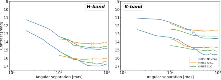
pixel resolution of 12.25 mas, which corresponds to the Nyquist sampling of SPHERE at 0.95 µm. The simulation implements a realistic model of the SPHERE instrument based on several inputs: VLT pupil, ExAO residuals, non-common path aberra-tions (NCPA), amplitude aberraaberra-tions, coronagraphic masks, and wavefront errors of the HiRISE injection optics. These values were derived from calibration measurements in SPHERE: imag-ing of the pupil for the amplitude maps, the Lyot stops,the coro-nagraphic masks, and ZELDA wavefront sensor measurements for the NCPA (Vigan et al. 2019). For the FIM, wavefront errors derived by the optical design software ZEMAX were used. For the residual atmospheric wavefront error we generated a series of 20 uncorrelated residual atmospheric phase screens using a Fourier-based AO simulation code (Fusco et al. 2006) with parameters representative of the SPHERE ExAO system, median observ-ing conditions, and a moderately bright AO star (R = 5). The three coronagraphic scenarios that we consider are the apodized-pupil Lyot Coronagraph (APLC;Soummer 2005;Carbillet et al. 2011;Guerri et al. 2011); the classical Lyot Coronagraph (CLC), implementable by not selecting the apodized pupil of the APLC; and a no-coronagraph option. All three of these options are avail-able in SPHERE without hardware interventions and are there-fore the only coronagraphs that are evaluated in this paper.

We then define the focal plane electric field for the fiber as the Gaussian E2 = e− 1 2( r σ) 2

, with radius r and σ as the standard deviation of the radius. In practice, fibers are often defined with a mode field diameter equal to MFD = 2ω, with E2 = e−(

r ω)2_. This means ω = √ 2σ and MFD = 2 √ 2σ. The corresponding intensity is given by I= |E2|2.

The fiber coupling efficiency represents how well the incom-ing wavefront projects onto the fundamental mode of the MFD. This can be calculated through an overlap integral with the two previous computed electric fields using the equation

η =    R E∗₁E2dA    2 R |E1|2dA R |E2|2dA , (1)

where η is the coupling efficiency, E1 and E2 are the complex

electric fields, and the integral is taken over all pixels of the field A. This equation is identical to the coupling efficiency equations inWagner & Tomlinson(1982) andJovanovic et al.(2017).

The sigma value of the Gaussian needs to be critically sized in terms of the scale of the PSF (in λ/D) to obtain an optimal coupling efficiency. We optimize the coupling efficiency for the parameter σ to derive the optimal size of the instrumental PSF, and therefore focal ratio F of the FIM at the fiber entrance plane. For a SPHERE-like pupil (14% secondary obscuration) we calculate, in a case without a coronagraph, that the optimally matching Gaussian has a σ= 0.504 λ/D. Using the APLC coro-nagraph this changes to the slightly smaller σ= 0.493 λ/D. We settle for an intermediate relation where σ = 0.5 λ/D to cover both scenarios. While taking the relation between MFD and σ into account, we calculate that to achieve the best average e

ffi-1.6 1.8 2.0 2.2 2.4 Wavelength [microns] 0.0 0.2 0.4 0.6 0.8 1.0

Coupling efficiency Pupil Amplitudes only

Pupil + AO Residuals

Pupil + AO Residuals + NCPA ("No Coronagraph") Pupil + AO Residuals + NCPA + Lyot Stop ("CLC")

Pupil + AO Residuals + NCPA + Lyot Stop + Apodizer ("APLC")

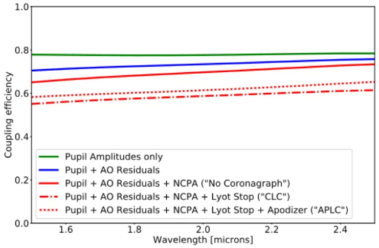
Fig. 1.Coupling efficiency as a function of wavelength for an off-axis companion to the host star. For a well-aligned fiber on top of the com-panion this shows the fraction of planet light that couples and propa-gates into the fiber. Contributions are added in one at a time to show their impact; highlighted in red are the three coronagraphic configura-tions considered in this paper.

ciency from 1.5 to 2.5 µm, considering the optimal MFD of the PSF and the factory-given MFD of the fiber, we need to provide a focal ratio F= 3.3 at the fiber. Details of the selected fibers are provided in Sect.2.5.2.

The F = 3.3 design, while optimal for injection into the fiber, does not lead to a practical opto-mechanical design, so we explored the impact of using slightly higher values of F. We measure that the relative loss in coupling efficiency for F = 3.4 and F = 3.5 is respectively, 0.1−0.8 and 0.6−1.8 percentage points, depending on the coronagraphic mode, which we con-sider acceptable. We decided to settle on a final design with F= 3.5.

For the fraction of planet light that couples into the fiber, we calculate the coupling efficiency for SPHERE (APLC, CLC, and no coronagraph) from 1.5 to 2.5 µm with 20 decorrelated realiza-tions of ExAO residuals generated with the AO code mentioned previously. To mimic an off-axis source (i.e., a planet) we use the complex PSF where the focal plane mask is not present. We extract the mean coupling efficiency and the average radial pro-file over the 20 realizations as a function of wavelength and use them for our simulator.

Figure1shows the coupling efficiency as a function of wave-length for the planet. The green line shows the coupling e ffi-ciency only using the SPHERE pupil amplitude, which includes amplitude aberrations measured directly by SPHERE. The blue line shows the coupling efficiency with simulated AO residuals added in. The lines in red additionally include the NCPA and HiRISE FIM wavefront error, and the effect of the coronagraphs. Due to the oversized spiders in the coronagraphic pupil stops, the coupling efficiency is significantly lower for the coronagraphic cases (CLC and APLC) than for the no-coronagraph case. The APLC mode gets higher coupling efficiency than the classical Lyot Coronagraph due to its apodized pupil optic that makes the PSF more Gaussian, which helps couple the light slightly more efficiently. Unfortunately, this increase in coupling efficiency is created by an amplitude mask in the pupil (apodized pupil) that blocks 57% of the incoming light, and therefore creates a major loss of photons that is not compensated by the increased cou-pling efficiency.

In Appendix B the dependence of the fiber injection e ffi-ciency on tip/tilt and lateral displacement in the focal plane is

1.5 2.0 2.5 Wavelength [microns] 10 6 10 5 10 4 10 3

fiber coupling efficiency

APLC

CLC

No Coronagraph

r= 245 mas r= 490 mas r= 980 mas

Coupling efficiency for star (excluding pupil transmission)

Fig. 2.Fraction of starlight coupling into the fiber as a function of wave-length at angular separations of 245, 490, and 980 mas. The curve and shaded regions show the average of the mean and 1σ boundary of the azimuthal statistics of 20 independent realizations of ExAO residuals.

shown. To remain at 99% and 95% of peak coupling efficiency a pointing accuracy of respectively 0.030 λ/D and 0.097 λ/D and a tilt accuracy of respectively 0.041 λ and 0.11 λ per λ/D (0.66 and 1.68◦ _{from normal incidence) is required for the}

non-coronagraphic case, which has the tightest tolerance.

As the planet lies in the speckle field surrounding the star, part of the starlight will also couple into the fiber at the loca-tion of the planet. To estimate this contaminaloca-tion, we recompute the overlap integral between the complex amplitude computed for the star in the two considered coronagraphic cases and non-coronagraphic case (E2) and a Gaussian placed at each location

in the simulated field of view (E1). With this procedure we obtain

a map that represents for each location in the field the fraction of starlight coupling into the fiber. For each PSF we also store the total flux with and without the coronagraphic mask and renor-malize the coupling efficiency of the starlight with this ratio to get the coupling efficiency with respect to the total of incom-ing light (i.e., relative to the flux before the focal plane mask) instead of the total remaining light in the focal plane. The results are summarized in Figs.2and3.

Figure2 shows the fraction of starlight from the halo that couples into the fiber as a function of wavelength and for three selected angular separations (i.e., 0.24500_{, close to the inner}

working angle of the coronagraph where the stellar halo should dominate; 0.4900_{, an intermediate point; and 0.98}00_{, where we}

expect the total flux to be dominated by the background). We see remarkably similar coupling of the stellar light at a level of about 10−5for all three options. Only very close to the star with the non-coronagraphic option do we see an increase in coupling efficiency, and therefore additional contamination from starlight with respect to the two coronagraphic options. In radial contrast profiles there is a more pronounced difference in the stellar sup-pression between coronagraph types (more than an order of mag-nitude difference at a few diffraction widths away from the star; see also AppendixAfor a comparison between raw contrast and the contrast achieved when sampling the PSF with a fiber). In Fig.2, where the focal plane is sampled by a single-mode fiber, this difference in contrast between coronagraphic modes is less apparent. This shows that the halo features for all three corona-graph options couple almost equally well and therefore resem-ble a Gaussian mode to the same extent. This effect has been explored in more detail by the work ofPor & Haffert(2020) and

Haffert et al.(2020) who propose and optimize a combination of 1 0 1 y [arcseconds]

APLC

Star

CLC

No coronagraph

Planet

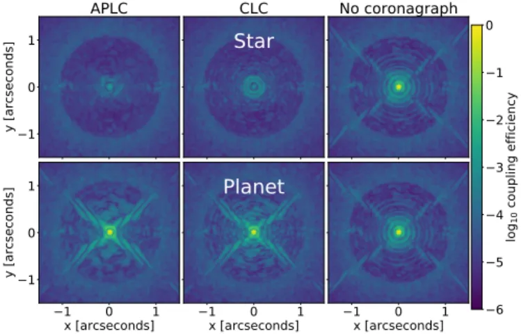
Fig. 3.Two-dimensional maps of the coupling efficiency as a function of separation, simulated at a wavelength of 1.6 µm and averaged over 20 realizations of atmospheric residuals. For the coronagraphic efficiencies of the star the inner ∼100 mas is additionally impacted by the transmis-sion loss caused by the focal plane mask. The coupling efficiencies for the star have been corrected to account for the light blocked by the focal plane mask as described in the main text.

coronagraph and single-mode fibers that minimizes the amount of starlight coupled into the fiber. The difference in transmis-sion and the inner working angles of the three coronagraphs are therefore important aspects to consider. As we show in Sect.4.4, performance is strongly driven by the total transmission of the system, so gaining in coupling efficiency is less critical than maximizing photons in the first place.

For completeness we show in Fig.3two-dimensional maps of the coupling efficiency for both the star and the planet. The stellar map assumes an aligned coronagraphic focal plane mask and can be used to read off the amount of starlight that ends up in the fiber, which is valid beyond 100 mas from the center. The planetary map has no focal plane mask applied and can be used to read off the amount of planet light that ends up in the fiber. For example, the top plots are read off at a certain separation (∼300 mas for β Pictoris b) to get the fraction of starlight cou-pling into the fiber (see Fig.2 for more exact values). Instead, for the bottom plots a fiber that is well aligned on the planet will couple with the efficiency that is visible at position x = 0, y = 0 (see Fig.1for more exact values).

Most noticeable, spatially, is the widened diffraction spikes from the spiders of the coronagraphic masks, which has a strong impact on the coupling efficiency for the planet.

2.5.2. Fiber transmission and extraction

To carry the light from SPHERE to CRIRES+ with a clean PSF and therefore line-spread function on the spectrograph, we use single-mode fibers. Single-mode ZBLAN fibers manufactured by Le Verre Fluoré (LVF) are ideally suited to cover both H and K bands with the highest possible transmission. Best matches within their catalog are the fibers with a core diameter of 6.5 µm, which have a single-mode cutoff at 1.48 µm, and a MFD of 7.2 µm at λ = 1.5 µm and 12.67 µm at λ = 2.5 µm. While sil-ica fibers designed for telecommunsil-ications could also satisfy the requirement of high transmission in H band very well, the ZBLAN fiber additionally enables observations in K band.

The fiber transmission of HiRISE is calculated from attenu-ation values provided by LVF for the selected SMF design and for a fiber length of 55 m. This distance is approximately equal

to that spanned by the UVES-FLAMES fiber connection on the VLT-UT2 (Pasquini et al. 2002; FLAMES P103 user manual2_),

which is similar to the setup that will be adopted for HiRISE. To reduce manufacturing risks and to facilitate the installa-tion of the fibers, the complete fiber assembly consists of three pieces joined with connectors, with losses of approximately 0.15 dB per connector. We assume a 2% loss for reflection on the input and output of the fiber.

The current design of the fiber extraction module (FEM) is based on four lenses to re-image the fiber onto the CRIRES+ focal plane and to match the F-number expected by CRIRES+ at the entrance of the spectrograph (i.e., F = 15) in a broad wavelength range from V to K band. This allows the operation of MACAO to keep the deformable mirror flat and provides high efficiency at the slit. These additional optical surfaces, together with the absorption in the medium of a heavy glass type required for one lens, combine to give a transmission factor of 0.80. 2.6. CRIRES+ spectrograph

Our baseline is that the high-resolution spectrograph that is used in combination with SPHERE is CRIRES+. CRIRES+ was installed in UT3 in early 2020, upgraded with a cross-disperser to increase the bandwidth, and with new low-noise detectors (Dorn et al. 2016). It provides a spectral resolution up to R = 100 000 in six different bands (Y to M), although not all bands are covered simultaneously. The bands of interest to HiRISE, H and K, are covered by four grating settings each to provide 100% wavelength coverage of the bands. In practice, a single setting will be used that covers approximately 68% of H band and 52% of K band, with gaps in the spectrum due to the way the three detectors cover the cross-dispersed orders.

The transmission of CRIRES+ was measured by its instru-ment team during the integration phase in Europe. The slit-independent transmission, but including the quantum efficiency of the detectors, is approximately 20% in H and K band (Seemann, priv. comm.). These values are approximate and sub-ject to change; final values will only be available when the instru-ment has been tested on-sky. Since they are currently the best available estimation, we use them for our simulations.

The 120 µm 0.200_{-wide, 10}00_{-long slit spans 3.1 pixels in}

width projected on the H2RG detectors. The read noise per pixel is approximately 7 electrons per readout and the dark current is 0.028 electrons per second3, with a gain that is 2.1 electrons per count. The dark current is scaled with the integration time and converted to dark noise by taking the square root. We assume that the light hits a 3.1 × 3.1 pixel area on the detector, and there-fore both the read noise and dark noise are scaled by a factor of 3.1 to give a conservative estimate of the noise per resolution element.

As we want to compare the combined HiRISE system with CRIRES+ standalone (i.e., where the slit is placed across star and planet, similar toSnellen et al. 2014) we determine the slit efficiency for both instrument configurations. Slit efficiencies were not included in the transmission measurement of CRIRES+ as the full slit was illuminated to be insensitive to these effects for the measurement of the transmission. The slit losses are small and constant with wavelength for HiRISE: the enclosed energy

2 _{https://www.eso.org/sci/facilities/paranal/}

instruments/flames/doc/VLT-MAN-ESO-13700-2994_p103. pdf

3 _{CRIRES+ forward simulator (CRIFORS): https://github.com/}

ivh/crifors 1.6 1.8 2.0 2.2 2.4 Wavelength [microns] 0.0 0.2 0.4 0.6 0.8 1.0 Slit efficiency

0.6" seeing, 0.2" slit oCRIRES 0.8" seeing, 0.2" slit oCRIRES 1.0" seeing, 0.2" slit oCRIRES 1.2" seeing, 0.2" slit oCRIRES

Fig. 4.Slit efficiency as a function of wavelength for seeing values of 0.600

, 0.800

, 1.000

, and 1.200

, extracted from the P95 CRIRES ETC. These values are not expected to change for CRIRES+.

diagrams of the optical design of the FEM indicate that more than 93% of the incoming light goes through the slit. Any AO degradation for HiRISE would translate into reduced fiber cou-pling efficiencies with unchanged slit losses.

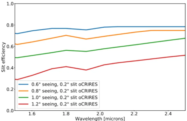
This is in contrast to CRIRES+ used in standalone, where slit losses are much higher and variable with seeing due to the lower order AO system MACAO. Figure4shows the fraction of enslitted light inside of the 0.200_{slit, referred to as slit efficiency,}

as a function of wavelength and for seeing values from 0.600 up to 1.200_{, extracted from the P95 CRIRES exposure time}

calcu-lator (ETC). We see that the slit efficiencies drop sharply with increasing seeing. At a seeing of 1.200the slit efficiency is almost halved compared to 0.800_{. If we look at a similar seeing difference}

for SPHERE we see a drop in Strehl, and therefore coupling e ffi-ciency, of about 15%. As a cross-check for the CRIRES ETC slit efficiencies we extracted the spatial profile at 2.3 µm from the data of Snellen et al.(2014; program ID 292.C-5017) and rotated this profile to get an artificial PSF. The enslitted energy within a 0.200 artificial slit corresponds within a few percent to the slit efficiency of the ETC at the same wavelength and DIMM seeing. As the MACAO system of CRIRES+ has not been sig-nificantly upgraded (and performance has to be revalidated on-sky) we assume that the slit losses of CRIRES can be directly used for our calculations of CRIRES+. In the remainder of the present work we use the average seeing of 0.800for CRIRES+ in standalone, as for the SPHERE ExAO simulations presented in Sect.2.5.1.

Lastly, the PSF profiles of CRIRES+ are taken from the ETC to simulate the strength of the stellar halo at the location of the planet. The previously mentioned slit efficiencies (enslitted energy) determine which fraction of this stellar light falls into the slit.

2.7. End-to-end transmission

Each transmission component is collected and multiplied to give the total transmission of the combination of instruments. Aver-aging over H- and K-band grating wavelength ranges we get the values in Table1. The total transmission in H and K band are 1.90% and 1.41%, respectively, for the non-coronagraphic case. The corresponding breakdown of the transmission into multi-ple components as a function of wavelength can be seen in Fig.5. In this figure we also see the impact of using two di ffer-ent dichroics and the regimes over which they are optimal. The

0.0

0.5

1.0

1.5

2.0

2.5

3.0

Total transmission [%]

Total transmission (top)

Total (DICH-H)

Total (DICH-K)

1.6

1.8

2.0

2.2

2.4

Wavelength [microns]

0

20

40

60

80

100

Transmission [%]

Transmission components (bottom)

Atmosphere

Telescope+SPHERE+HiRISE (DICH-H)

Tel+SPHERE+HiRISE (DICH-K)

Fiber injection

Fiber transmission incl. couplers

CRIRES+ incl. slitloss

Fig. 5.Upper panel: total transmission for DICH-H and DICH-K (optimized respectively for K and H band). Lower panel: breakdown of transmis-sion into components. Fiber injection and transmistransmis-sion based on the no-coronagraph case.

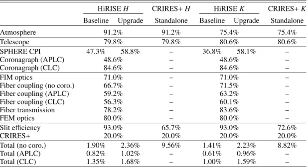
Table 1. Average end-to-end transmission in H and K bands broken down into individual components.

HiRISE H CRIRES+ H HiRISE K CRIRES+ K

Baseline Upgrade Standalone Baseline Upgrade Standalone

Atmosphere 91.2% 91.2% 75.4% 75.4% Telescope 79.8% 79.8% 80.6% 80.6% SPHERE CPI 47.3% 58.8% – 36.8% 58.1% – Coronagraph (APLC) 48.6% – 48.6% – Coronagraph (CLC) 84.6% – 84.6% – FIM optics 71.0% – 71.0% –

Fiber coupling (no coro.) 66.7% – 71.5% –

Fiber coupling (APLC) 59.2% – 63.2% –

Fiber coupling (CLC) 56.3% – 60.1% –

Fiber transmission 78.2% – 83.6% –

FEM optics 80.0% – 80.0% –

Slit efficiency 93.0% 65.7% 93.0% 72.6%

CRIRES+ 20.0% 20.0% 20.0% 20.0%

Total (no coro.) 1.90% 2.36% 9.56% 1.41% 2.23% 8.82%

Total (APLC) 0.82% 1.02% – 0.61% 0.96% –

Total (CLC) 1.35% 1.68% – 1.00% 1.59% –

Notes. The baseline case uses current SPHERE dichroics. The upgrade case assumes a clear plate instead of less efficient SPHERE dichroics. For coronagraphic and fiber coupling transmission factors only one of each applies.

highest transmission is achieved by using CRIRES+ alone, which has an end-to-end transmission of 9.56% and 8.82% in Hand K. Focusing on HiRISE the highest transmission is seen in the non-coronagraphic mode, then the CLC mode which only has a pupil stop and focal plane mask, and the poorest trans-mission is seen for the APLC, which includes an additional

apodizing pupil mask. The transmission differences are purely driven by the change in injection efficiency and the additional light blocking of the coronagraphic masks. Swapping the exist-ing dichroic for a clear plate that conserves the beam path and optical path length will give 24% in H and 58% in K band of additional light and is broken down in the upgrade column.

2.8. Background thermal radiation

The majority of the path of the full instrument combination is at an ambient temperature of about 14◦C. Only inside of CRIRES+ is there a cryogenic vessel with the slit acting as a cold field stop. The slit sees the upstream thermal radiation, which comes from the re-imaging optics for the fiber extraction unit, the front surface of the fibers, and the thermal radiation transmitted from the SPHERE side. In the case of mirrors, the light that is not reflected is mostly absorbed so this directly gives us the emis-sivity of the mirror. In the case of lenses or dichroics, the light that is not transmitted is mostly reflected. The reflected paths look into the instrument, which is at ambient temperature, and so the emissivity is (1−transmission) for these optical elements. The dominant thermal components will therefore be the poorest transmitting or reflecting optics that are at room temperature.

In the case of SPHERE and HiRISE this is the IRDIFS dichroic and the coronagraph optics. As the Lyot apodizer and the Lyot stop have a chromium mask, the fraction of light that is not transmitted is reflected and therefore it sees the surrounding warm surfaces. We assume that only the light that geometrically fits into the 6.5 µm core of the fiber and in the angular cone that is spanned by the numerical aperture can pass through the fiber.

On the CRIRES+ side, most of the optical path is cooled, but the fiber face can in the worst case be considered a half-open cylindrical cavity with emissive walls, and can therefore be considered to have strong emissivity and to be the dominant background source on the CRIRES+ side as seen from the cold slit. In our simulation we therefore implement SPHERE at an emissivity of 0.7, approximating the amount of light lost in the upstream branch, and the fiber-end at a very conservative emis-sivity of 1.0. For the SPHERE side we integrate background light over a circular surface with a diameter of 6.5 µm and a cone with a half-angle of arcsin(0.17), derived from the F-number. For CRIRES+, a larger part of the face of the fiber is visible from the slit than just the core. The 120 µm slit width back-projected onto the fiber gives a width of 28 µm, which is used as the emit-ting surface. We also use a cone with a half-angle of arcsin(0.17) as the emissive angular area. Using Helmholtz reciprocity, the surface area and the area in the cone are multiplied to give us the amount of light arriving at the slit, which corresponds to the thermal background radiation considered in the simulation. 2.9. Simulation of the final spectra

We use the source spectra scaled by the simulated detector inte-gration time (DIT) and multiply them by all transmission factors down to the CRIRES+ detector, while the background light from the sky, SPHERE, and fiber are transmission-corrected from their respective locations of origin. The starlight, planet light, and atmospheric radiance are multiplied by the surface area of the telescope, which is 49.28 m2_{, considering the 8 m telescope}

and 14% secondary obscuration and the width of each wave-length bin.

A science signal is made from the sum of the stellar halo, planet light, Earth’s atmospheric radiance, dark current, back-ground from fiber and backback-ground from the SPHERE instru-ment as measured at the CRIRES+ detectors over each 3.1 × 3.1 pixel area. We also construct a reference signal that contains all the components except for the planet light, which in prac-tice will be obtained using multiple reference fibers (4+) that sample the PSF, background, and sky at different locations in the focal plane. While speckles have a chromatic dependence, it is a low-order effect, which is suppressed by our high-pass

filtering. The fibers sampling the PSF provide multiple refer-ences for the starlight. Additionally, a reference spectrum can be taken by putting the star on the science fiber. The detailed data analysis of the HiRISE data will be studies in future work. For each spectral bin of both the science and reference signal we draw from a Poisson distribution with its parameter λ as the total flux, and sum it with read noise drawn from a normal distribution. The final planetary spectrum to be analyzed is the difference between the science signal and the reference signal. For CRIRES+ standalone the impact of SPHERE and HiRISE is excluded from these calculations.

3. Performance for known targets

3.1. Simulations and signal-to-noise ratio estimation

The main scientific driver for the HiRISE project is the detailed characterization of known companions at small separations, where the detection and subsequent characterization of faint companions are typically limited by the stellar halo and by the high level of residuals after post-processing (e.g.,Cantalloube et al. 2015). We first estimate the performance of the combina-tion of SPHERE and CRIRES+ in this specific regime by sim-ulating known exoplanetary systems and evaluating the S/N on particular species expected in their atmospheres.

The known systems that we evaluate in this section are HIP 65426 (Chauvin et al. 2017b), β Pictoris (Lagrange et al. 2009), PDS 70 (Keppler et al. 2018), and 51 Eridani (Macintosh et al. 2015). These targets are planets (in contrast to brown dwarfs), relatively close in angular separation to their star and visible from the VLT. Their assumed physical and observa-tional properties are provided in Table2. To avoid interpolations in the grids of stellar and sub-stellar atmospheric models, for the stars and planets we use the models with the closest available Teff and log g. We simulate the realistic spectra for each of the

targets with a varying integration time. Then we perform a cross-correlation analysis of the simulated total spectra, which includes all molecular contributions and noise, against both the input planetary spectrum and the spectral contribution of individual molecular species (H2O, CO, and CH4).

The simulations are performed for several instrumental con-figurations. First we consider CRIRES+ in standalone mode (i.e., without the HiRISE coupling). In this case only the tele-scope, atmosphere, and CRIRES+ transmission from Table1are considered in the simulation of the spectra. Then, for HiRISE we consider three different setups that include different types of coronagraphs: no coronagraph, APLC, and CLC. For the HiRISE simulations, the simulation of the spectra include the additional contributions in transmission from SPHERE, the FIM optics, the fiber coupling, and finally the FEM optics.

For this analysis we select the wavelength range available to each CRIRES+ grating setting, which we extracted from the CRIFORS simulator. Both the observed and comparison spec-tra are preprocessed by removing the low-order (continuum) through a high-pass filter using a fast Fourier transform, as commonly done. This filtering step can be skipped if the full SPHERE/HiRISE/CRIRES+ combination can be spectrally cal-ibrated. The S/N of the cross-correlation is then calculated using the matched filter approach (Ruffio et al. 2017) where the maxi-mum likelihood S/N is defined by

S/Nv= Pk idimv,i/σ2i q Pk im2v,i/σ2i , (2)

Table 2. Planetary system parameters used as input for simulations.

Star Companion

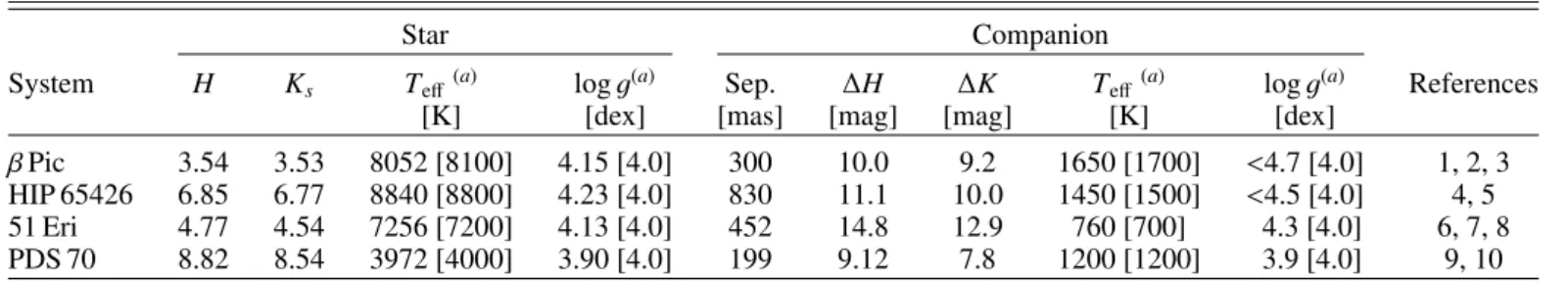
System H Ks Teff (a) log g(a) Sep. ∆H ∆K Teff(a) log g(a) References

[K] [dex] [mas] [mag] [mag] [K] [dex]

β Pic 3.54 3.53 8052 [8100] 4.15 [4.0] 300 10.0 9.2 1650 [1700] <4.7 [4.0] 1, 2, 3 HIP 65426 6.85 6.77 8840 [8800] 4.23 [4.0] 830 11.1 10.0 1450 [1500] <4.5 [4.0] 4, 5 51 Eri 4.77 4.54 7256 [7200] 4.13 [4.0] 452 14.8 12.9 760 [700] 4.3 [4.0] 6, 7, 8 PDS 70 8.82 8.54 3972 [4000] 3.90 [4.0] 199 9.12 7.8 1200 [1200] 3.9 [4.0] 9, 10

Notes.(a)_{The T}

eff and log g values from the literature are reported on the left side of the columns, while the values used for the models in the simulation are reported between brackets on the right side of the columns.

References. (1)Bonnefoy et al.(2013); (2)Lagrange et al.(2019); (3)Chilcote et al.(2017); (4)Chauvin et al.(2017a); (5)Cheetham et al. (2019); (6)Macintosh et al.(2015); (7)Samland et al.(2017); (8)Rajan et al.(2017); (9)Keppler et al.(2018); (10)Müller et al.(2018).

where diis the high-pass filtered observed data, mv,iis the

high-pass filtered model shifted at radial velocity (RV) v and resam-pled at the same wavelengths as di, and σiis the estimated noise

of the data di(before the high-pass filter). The sums from i= 0

to k are over each spectral data point. The calculation is repeated for a range of radial velocities v and the final S/N is evaluated at the input RV, which is equal to zero in the case of these simula-tions.

The noise in the data is derived by quadratically adding up all the known contributions of noise. In the case of the simulation the exact noise contributions are perfectly known, but the case with real data will have to be handled differently. In HIRISE, in addition to the science fiber where the planet signal will be injected, we foresee the addition of reference fibers that will sample the stellar speckle field at locations around that of the planet. These reference signals will then be used in the data anal-ysis for subtracting part of the stellar contribution and estimating the noise in the data.

As detailed in Sect.2.6, CRIRES+ offers several grating set-tings that cover a full band in up to four distinct observations. An initial set of cross-correlations on all H- and K-band set-tings separately revealed that the S/N values do not vary much between grating settings for the models that we use, even when focusing on individual atmospheric species, presumably because the amount and the strength of the molecular lines that are cov-ered do not change significantly between grating settings within the same band. Hereafter we therefore only consider H_1_4 and K_1_4 settings to accelerate calculations.

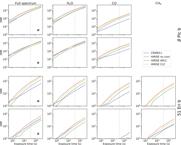
3.2. Performance as a function of exposure time

For a quantitative comparison of CRIRES+ standalone with HiRISE, we first evaluate the expected S/N as a function of the exposure time for the brightest and faintest planets in our sam-ple, namely β Pictoris b and 51 Eridani b. The simulated spectra are compared to both the noiseless input planet spectrum and to individual spectral templates for molecules expected in the atmo-spheres of the two planets. The results are plotted in Fig.6 for the molecules that are expected a priori to have strong features, which are H2O and CO for β Pic b and H2O, CO, and CH4 for

51 Eridani b.

We first look at the S/N computed when comparing the sim-ulated spectra with the input noiseless planet spectrum. We see a clear increase in S/N as a function of integration time in all instrumental configurations. Indeed, β Pictoris b and 51 Eridani b have relatively bright host stars, H = 3.54 and H = 4.77, and are at very close angular separation from their host, 300 mas

and 452 mas, respectively. Therefore, for both systems the noise is strongly dominated by the photon noise of the stellar halo, resulting in a slow increase of the S/N with exposure time. As we show in Sect.3.3, the noise regime has a strong impact on performance.

In this comparison we also see that HiRISE without coron-agraph almost always provides a gain of at least a factor&1.4 in S/N with respect to CRIRES+. Assuming that the regime is indeed photon noise limited, this roughly translates to a gain of a factor of &2 in exposure time to reach the same S/N. It is only at short exposure times (typically <100 s) that in some cases CRIRES+ provides a better S/N than HiRISE as the short integration times can put the systems in the read noise limited regime where higher transmission is more important. We note that for the β Pic host star, HiRISE without corona-graph can be surpassed by HiRISE with coronacorona-graph. We ana-lyze the effect of the coronagraph in HiRISE in more detail in Sect.4.3.

The same results are observed when looking at individual molecules. We see that it is possible with HiRISE without coro-nagraph to reach the same S/N in a fraction of the observing time as CRIRES+ reaches in one hour. For H2O in H band we see that

the same S/N achieved by CRIRES+ in 1 h of integration time is reached in only 1560 s with HiRISE, corresponding to a factor of 2.3 gain, while for CO the same value as CRIRES+ is reached in only 300 s, corresponding to an even higher gain (a factor of 12). In K band, HiRISE provides gains of approximately a factor of 11 for CO and no clear improvement for H2O.

CH4is barely detected in the atmosphere of 51 Eridani b with

CRIRES+ in the H band, while it appears to be easily detectable with HiRISE provided typical exposure times of longer than a few hundred seconds. In K band the detection appears easier for CRIRES+, but even longer exposure times than in H band are required.

Interestingly, the S/N values reached for H2O are very close

to the values reached when comparing to the full input spec-trum. H2O is the dominant contributor in terms of spectral lines

in the atmospheres of these planets, in H and in K band, so it has a higher weight in the matched filtering and therefore drives the final value of the S/N. We also note that CO appears barely detectable in K band for 51 Eridani b, which is surprising considering the strong CO overtones starting at 2.29 µm. This absence of detection is likely due to the instruments starting at 1.9−2.0 µm and to the general faintness of the planet in this band (K= 17.4).

We conclude that even though the global transmission of HiRISE is low, it provides a significant gain of observing time

10

10

10

10

SNR

H

Full spectrum

CRIRES+

HiRISE no coro

HiRISE APLC

HiRISE CLC

10

10

10

10

H

O

10

10

10

10

CO

CH

10

10

10

10

SNR

K

10

10

10

10

10

10

10

10

10

10

10

SNR

H

10

10

10

10

10

10

10

10

10

10

₁₀

₁₀

Exposure time (s)

10

10

10

SNR

K

10

₁₀

₁₀

Exposure time (s)

10

10

10

10

₁₀

₁₀

Exposure time (s)

10

10

10

10

₁₀

₁₀

Exposure time (s)

10

10

10

Pi

c b

51 Eri b

Fig. 6.Estimation of the S/N as a function of exposure time for the observation in H and K band of β Pictoris b (top rows) and 51 Eridani b (bottom rows) with CRIRES+ (blue lines) and HiRISE in different coronagraphic configurations: no coronagraph (red lines), APLC (green lines), and CLC (yellow lines). The S/N is computed with a matched filtering approach (see Sect.3.1) comparing the simulated spectra with the noiseless input planet spectrum (Full spectrum column) and with noiseless spectral templates for molecules (H2O, CO and CH4). The vertical dotted lines indicate

1 h integration time.

with respect to CRIRES+. The exact values provided in this section are model dependent and some molecules might be more pronounced in theory than seen in reality around these targets, but the order of magnitudes will hold whatever the model, as will the relative gains between HiRISE and CRIRES+.

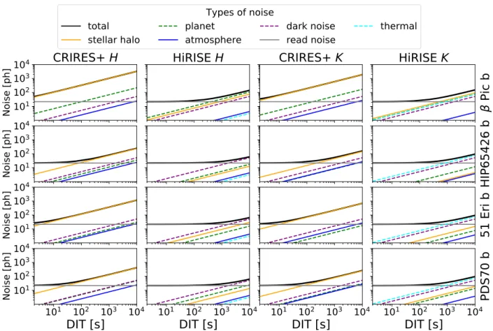
3.3. Noise breakdown

The performance of HiRISE is strongly dependent on the noise regime in which the system is used, which itself depends on the brightness of the target that is observed. To illustrate the change in noise regime when using HiRISE, we show the square root of the mean of the variance within a certain band (the average noise per resolution element). In this simulation we consider the four planets presented in Sect.3.1, which span a wide range of visual magnitudes in H and K band: β Pictoris b (H= 13.5, K = 12.7), PDS 70 b (H = 17.9, K = 16.3), HIP 65426 b (H = 18, K= 16.8), and 51 Eridani b (H = 19.6, K = 17.4). We generate spectra for the four targets and we extract the noise for each of the noise sources.

Figure7shows the average noise per resolution element for each noise contribution in the simulated spectra for CRIRES+

and HiRISE without coronagraph as a function of time. The figure demonstrates that for each planet observed with CRIRES+ one of the strongest dominating noise sources is the Poisson noise on the stellar halo, which is therefore the performance lim-iting factor, and any suppression of this noise will directly pro-vide a gain in S/N.

When using SPHERE in combination with CRIRES+ the noise regime changes drastically. In most cases, even without a coronagraph, HiRISE suppresses the stellar halo to a point where, due to the reduced transmission, the noise terms that orig-inate in the sensor become relatively more important and the stellar halo noise is no longer the dominant component. In H band the dominant noise source becomes either dark noise, read noise or noise on the planet itself depending on the target bright-ness, separation, planet to star contrast and integration time. For the brightest stars like β Pictoris, the stellar halo in addition remains an important noise contributor. In K band the dominant noise sources are read noise, dark noise and thermal noise from SPHERE, with in addition the stellar halo for the very brightest stars. In general, after starlight suppression several noise terms are within one order of magnitude of each other. To avoid the read noise limited regime a detector integration time of at least

10

10

10

10

Noise [ph]

CRIRES+ H

Types of noise

total

stellar halo

planet

atmosphere

dark noise

read noise

thermal

HiRISE H

CRIRES+ K

HiRISE K

10

10

10

10

Noise [ph]

10

10

10

10

Noise [ph]

10

₁₀

₁₀

₁₀

DIT [s]

10

10

10

10

Noise [ph]

10

₁₀

₁₀

₁₀

DIT [s]

10

DIT [s]

10

10

10

10

DIT [s]

10

10

10

Pi

c b

HIP65426 b

51 Eri b

PDS70 b

Fig. 7.Breakdown of the noise into individual sources vs. detector integration time for four planets observed using CRIRES+ and HiRISE without coronagraph. The noise is effectively the average noise per resolution element within a certain band and is expressed in photons.

∼1000 s is needed for HiRISE. Detector integration times around this duration would also provide a reduced risk of saturation and less spectral blurring than much longer exposures. For planets at 100 mas around bright stars (H= 3) the 62 000 electrons full well capacity is reached in the science fiber without a corona-graph in 8000 s DIT for H band (even when assuming the light is concentrated into 3 pixels per resolution element). For 50 mas it is reached in 600 s with the stellar halo as limiting factor. In Kband these limits are respectively 4000 and 250 s. Taking the 42 000 electron per pixel limit for the linear regime, this level is reached in a fractionally shorter time (68%), which requires exposures that are as short as 3 min at 50 mas in H band. Fainter host stars allow for longer DITs.

This noise breakdown illustrates the two main factors that drive the performance of high-contrast systems in general, and is especially applicable for systems coupled with high-resolution spectroscopy: the reduction of the stellar contribution at the loca-tion of the planet using ExAO and coronagraphy, and the global transmission of the system. Without the former, the performance is largely driven by the photon noise from the star, the situation in which any ideal system should be, but the noise level will be high compared to the faint signal of the planetary companions that we seek. Conversely, without the latter the other systematic effects in the system will start to become limiting factors com-pared to the photon noise.

4. Discovery potential

We anticipate the discovery of more directly imaged (or image-able) planets in the near future. The current SPHERE GTO survey SHINE (Chauvin et al. 2017a) has discovered

sev-eral potential planetary candidates at small angular separations that are difficult to confirm with current imaging capabilities (SHINE consortium, priv. comm.). Additionally, the ESA/Gaia mission (Gaia Collaboration 2016) is expected to release thou-sands of exoplanet candidates discovered through the astromet-ric method out to separations of 5 AU and distances of 500 pc (Perryman et al. 2014) in its final data release. Both categories of planetary candidates are found in regimes that are pushing the limits of what the current generation of direct imagers can do, but provide a crucial view on an unprobed range of parameter space (i.e., planets closer to their star, and older host stars).

It is therefore interesting to look at the expected performance of HiRISE as a planet discovery or confirmation instrument. With a sparse field of view of a few single resolution elements, HiRISE certainly cannot be used to blindly search for planetary companions. However, with prior knowledge of the location of a candidate, HiRISE can become a powerful confirmation instru-ment and provide important high spectral resolution data on con-firmed companions.

In this section we compare the detection performance of HiRISE and CRIRES+ (Sect. 4.1) for unseen companions, in particular as a function of the stellar host brightness (Sect.4.2). Then we study in more detail for HiRISE the impact of the coro-nagraph choice (Sect.4.3) and of the overall transmission of the system (Sect.4.4).

4.1. Detection performance

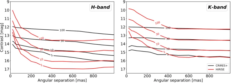
We determine detection limits for HiRISE and CRIRES+ stan-dalone by simulating observed spectra for a grid of planets in a range of separations (20 ≤ r ≤ 1000 mas) and contrasts (delta

0

200

400

600

800

Angular separation [mas]

9

10

11

12

13

14

15

16

17

Contrast [mag]

H-band

0

200

400

600

800

Angular separation [mas]

9

10

11

12

13

14

15

16

17

K-band

Fig. 8.Signal-to-noise ratio as a function of contrast (∆m) and separation for HiRISE without a coronagraph (red contour lines) and CRIRES+ standalone (black contour lines). The simulation is performed for a β Pictoris-like host star with a 1200 K planet and 2 h of integration time. The S/N is computed with a matched filtering approach (see Sect.3.1) comparing the simulated spectra with the noiseless input planet spectrum. For this combination of parameters the S/N inward of 400−500 mas is dominated by the noise on the stellar halo. Outside of 400−500 mas it is limited by dark and read noise.

magnitudes of 7.5 ≤ ∆m ≤ 16), and located around host stars with H-band magnitudes from 3 to 9. We set the integration time to 2 h and calculate the S/N through a matched filter approach with the noiseless input planet spectrum. Although optimistic, this comparison with the input spectrum enables us to investi-gate the ultimate performance of the system.

The results are presented in Fig.8with contours at fixed val-ues of S/N for a bright host similar to β Pictoris (A5V, H = 3.5) and a temperature of 1200 K. Additional results for a fainter host star similar to HIP 65426 (A2V, H = 6.9) are provided in AppendixC. In this figure only the HiRISE non-coronagraphic setup is shown in comparison to CRIRES+ as it is the mode that provides the best performance and best inner working angle (see Sect.4.3). As the noise breakdown has demonstrated, the S/N of CRIRES+ is dominated by the stellar halo at most sep-arations. At separations larger than 1000 mas where the noise for HiRISE is dominated by read, dark and instrumental ther-mal noise (depending on the band), CRIRES+ logically provides better performance than HiRISE. Likewise, at separations below 50 mas where the stellar halo starts to dominate even for HiRISE and where the planet and source are effectively unresolved, the additional transmission of CRIRES+ beats the HiRISE non-coronagraphic mode, although in this case the RV signal of the planet needs to be probed in time to disentangle star and planet light and the exposure time sufficiently short to avoid saturation on the star. The behavior at small separations is similar for the faint H= 6.8 host (see Fig.C.1).

Even so, in the intermediate range from 50 mas up to several hundred mas (800 mas for both bright and faint) HiRISE pro-vides a substantial gain in sensitivity. At 200 mas in the H band, there is a 1.3 mag gain in contrast at which an S/N of 5 is reached. Conversely, looking at the S/N at a contrast ∆m = 15 and separa-tion of 200 mas, we can get an increase in S/N of a factor of ∼4, equivalent to a gain in observing efficiency of about 16 times. For the faint host star in H band we see a gain of 1.0 mag in con-trast at 200 mas, and at∆m = 13.75 and a separation of 200 mas we see an increase in S/N of a factor 2.4, which translates into a gain in observing efficiency of a factor 5.8.

In K band around bright hosts, HiRISE narrowly outper-forms CRIRES+ in a window between 400 and 650 mas, with a

gain of 0.2 mag at 600 mas for an S/N of 5. For fainter host stars, the window disappears for planets at 1200 K. Despite the use of high-throughput fibers, the performance of HiRISE is clearly limited in K band with respect to CRIRES+ in standalone. At low overall throughput, the contribution of the thermal noise stays an important limitation, which cannot be compensated by the gain from ExAO and spatial filtering by the fiber.

With a planet temperature of 1700 K the highest gains seen in H and K band are 1.2 mag at 300 mas and 0.6 mag at 500 mas respectively for host stars as bright as β Pictoris. For fainter stars like HIP 65426 the highest gains at 200 mas are respectively 0.8 and 0.1 mag. The corresponding plots for these values are not shown but the numbers are provided as a reference.

4.2. Relation with apparent magnitude of host

The dependence of the performance on the host magnitude is an important parameter. To analyze how the performance varies with the host NIR magnitudes, we repeat the same S/N calcula-tions as before, but vary the magnitude of the A5V host star in a range from 3 to 9. Figure9shows the contrast at which an S/N of 5 is reached for a two-hour integration time and a 1200 K com-panion, as a function of angular separation and host star magni-tude. Again this comparison is between CRIRES+ and HiRISE without a coronagraph. This figure shows the trends previously identified, with HiRISE giving enhanced performance from sep-arations of 50 mas to at least 400 mas in H band, even for hosts as faint as H = 8.5. For stars that are brighter than the above-mentioned magnitudes the outer limit extends beyond 400 mas, while the inner limit remains similar. For K band this region spans from about 400 mas to 700 mas for stars with K = 3.5, but even in this region the gain provided by HiRISE is extremely limited. At K= 4.5 the region becomes very narrow and the con-trast improvement is only marginal. The gray dotted line shows where the performance of both instruments is equal and provides an overview of the regime that HiRISE should operate in (for the given simulation parameters), which is inward of this line.

For HIP 65426 b we see that CRIRES+ has a small advan-tage over HiRISE in H band. With a separation of 830 mas and a moderately faint host star, the noise is initially dominated by the stellar halo but not as strongly as with candidates closer to the