Publisher’s version / Version de l'éditeur:
Vous avez des questions? Nous pouvons vous aider. Pour communiquer directement avec un auteur, consultez la première page de la revue dans laquelle son article a été publié afin de trouver ses coordonnées. Si vous n’arrivez pas à les repérer, communiquez avec nous à PublicationsArchive-ArchivesPublications@nrc-cnrc.gc.ca.
Questions? Contact the NRC Publications Archive team at
PublicationsArchive-ArchivesPublications@nrc-cnrc.gc.ca. If you wish to email the authors directly, please see the first page of the publication for their contact information.
https://publications-cnrc.canada.ca/fra/droits
L’accès à ce site Web et l’utilisation de son contenu sont assujettis aux conditions présentées dans le site LISEZ CES CONDITIONS ATTENTIVEMENT AVANT D’UTILISER CE SITE WEB.
25th IAHR International Symposium on ICE, 2020-11-25
READ THESE TERMS AND CONDITIONS CAREFULLY BEFORE USING THIS WEBSITE. https://nrc-publications.canada.ca/eng/copyright
NRC Publications Archive Record / Notice des Archives des publications du CNRC :
https://nrc-publications.canada.ca/eng/view/object/?id=0bbd9913-b0dc-4462-bdbc-0f129e2ca419 https://publications-cnrc.canada.ca/fra/voir/objet/?id=0bbd9913-b0dc-4462-bdbc-0f129e2ca419
NRC Publications Archive
Archives des publications du CNRC
This publication could be one of several versions: author’s original, accepted manuscript or the publisher’s version. / La version de cette publication peut être l’une des suivantes : la version prépublication de l’auteur, la version acceptée du manuscrit ou la version de l’éditeur.
Access and use of this website and the material on it are subject to the Terms and Conditions set forth at Numerical simulations of naval vessel collisions with ice
1
Numerical Simulations of Naval Vessel Collisions with Ice
R. Gagnon1, J. Wang2, D. Seo3 and J. Mackay4
1, 2, 3 OCRE/NRC; 4 DRDC
1, 2, 3 St. John’s, NL, Canada; 4 Halifax, NS, Canada
1Robert.Gagnon@nrc-cnrc.gc.ca, 2Jungyong.Wang@nrc-cnrc.gc.ca,
3 DongCheol.Seo@nrc-cnrc.gc.ca, 4John.Mackay2@forces.gc.ca
Numerical simulations (using LS-DynaTM) were initially conducted to show two scenarios for a naval vessel, one where little-to-no-damage occurs during an ice collision and the other where substantial damage occurs. NRC’s crushable-foam ice model was used for all simulations. One instance of the first scenario corresponded to the vessel moving at a given vessel speed of 1.5 m/s and experiencing a bow-side collision with a block-shaped ice mass of approximately 181 tonnes that caused a relatively small amount of plastic damage to the vessel’s hull (i.e. a wide-area shallow-depth plating dent with depth of ~ 11 mm). In contrast, the second scenario corresponded to the vessel colliding at the same speed with a 524 tonne similar-shaped ice mass at the same hull location that caused extensive, non-holing, plastic damage to the vessel grillage. That is, the hull plating experienced substantial plastic indentation (~ 60 mm) and the stiffener and frame in the region of impact underwent bending and buckling. Following those simulations, others were performed using progressively smaller ice masses in order to determine what the size of an ice mass would be that would cause no damage at all to the vessel. The results indicated that some level of damage, albeit diminishingly small, occurred (in a linear trend) as the ice masses and associated peak loads get smaller until eventually an ice mass of 8 tonnes produced no damage at all, where the peak load was 25 kN. The next ice-mass size up from that was 17 tonnes, that produced a tiny amount of damage during a simulation. An important observation from all the simulations concerns where the ice impact occurs with respect to supporting stiffeners and frames behind the plating. This can influence the peak loads and pressures that occur, and the extent of local damage. The 524 tonne ice mass collision simulation yielded average and peak contact pressures that were in reasonable agreement with average and hard-zone pressure values obtained in large double pendulum ice impact lab tests. This, and favorable comparisons with other lab and field data, bolster confidence in the ice model used.
25
thIAHR International Symposium on Ice
2
1. Introduction and Background
Marine transportation in Arctic regions is seriously affected by the presence of glacial and sea ice masses. Of concern for ships (including naval vessels) are bergy bits and growlers (house-sized and car-(house-sized glacial ice masses) and sea ice masses (e.g. a chunk of multi-year sea ice, a chunk from a dense sea ice rubble field or from a consolidated ridge, individual floes or smaller portions broken from floes). Detection of ice masses is sometimes difficult using marine radar in rough sea states. Should ice make contact with a ship's hull, the impact forces will depend on the masses of the vessel and ice, the hydrodynamics of the interaction, the ship structure, the shape of the ice mass and its local crushing properties.
Numerical simulations of a naval vessel colliding with ice were conducted. The simulations involved collisions with ice masses of varying size at the side of the vessel’s bow. Some scenarios entailed relatively mild collisions (≤ 514 kN peak impact load) with a single ice mass (in the range of 8-181 tonnes) where moderate to little damage (or no damage in one case) to the vessel occurred. The other scenarios involved damaging, but non-holing, collisions with ice masses (in the range 98-524 tonnes) where greater permanent indentation of the vessel’s grillage occurred and where peak loads were in the range 200-769 kN. Hit location, with respect to stiffeners and frames, was a factor. The simulations were run at NRC/OCRE STJ using NRC hardware (HP Z840 Workstation) and licensed LS-DynaTM software. NRC’s validated ice model was used for the simulations. The results are presented below.
2.0. Numerical Simulations of a Naval Vessel Colliding with Ice Masses
As mentioned above, the purpose of the simulations was to show various cases of a naval vessel colliding with ice, some cases where mild damage (or no damage) occurred and the others where significant permanent non-holing damage was done to the grillage. The strategy used to accomplish this was to utilize similar-shaped ice masses, of various sizes, to perform the collision simulations. The initial masses of the ice objects needed to fit these requirements had to be determined from a few trial-and-error simulations so that for the chosen vessel speed of 1.5 m/s the largest ice mass (~ 524 tonnes) caused obvious damage to the grillage and a smaller ice mass (~ 181 tonnes) caused substantially less damage. The trial-and-error tactic was necessary because the shape of the slender naval vessel, where the bow expanded at about 10o from the vessel’s length axis, was radically different from other vessels and structures for which ice-impact simulations had been conducted before by the NRC/OCRE simulation team. The initial trial runs were ‘dry’ runs that did not involve hydrodynamic effects.
2.1. Naval Vessel and Impacted Hull Segment Description
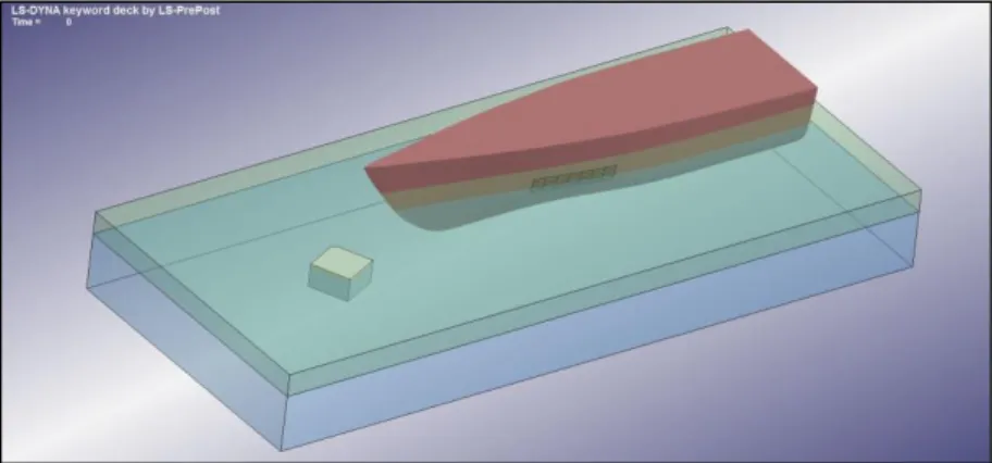
Figure 1 shows the full meshed volume used in the simulations. The front half portion of the vessel that was generated by NRC from the IGES file that was supplied by DRDC is visible. DRDC also supplied a report which contained all relevant information necessary to describe the properties of the hull portion which NRC had decided that ice impacts would most appropriately occur in the simulations. Table 1 gives information on the vessel and Table 2 gives properties of the target hull segment. Figure 2 shows the vessel body plan.
2.2. Bulk-Ice Mass and Target Ice-Knob
An ice mass is shown in Figure 3. In this instance the bulk-ice mass represents a block-shaped ice feature such as a glacial ice growler, a chunk of multi-year sea ice or a chunk from a dense sea ice rubble field or from a consolidated ridge. The hemispherical ice mass (a.k.a. the ‘ice-knob’) is attached at one of the corners of the ice mass feature. A validated ‘crushable foam’ material model (Gagnon and Derradji-Aouat, 2006) was used to characterize the ice-knob. To do this, LS-Dyna’s material model MAT_63 was used with the following inputs: Density = 870 kg/m3, Young’s Modulus = 9 GPa, Poisson’s Ratio = 0.003, Tensile Stress Cutoff = 800 MPa,
3
and the Yield Strength versus Volumetric Strain curve the same as that used by Gagnon and Derradji-Aouat (2006). Table 3 gives information on the characteristics of the initial ice masses used for the simulations.
2.3. Meshing Considerations and Simulation Strategy
Following the methods of Gagnon and Wang (2012), the main large objects that do not interact with anything other than water and air, i.e. the vessel and the bulk-ice mass, are given a large, but adequately refined, mesh size that matches the mesh size of the water and air domains. On the other hand, the ice-knob and deformable grillage must be finely meshed, since their interaction volume is much smaller, in order to capture the appropriate behaviors during the impacts. These relatively small and finely meshed objects do not have to interact with the water and air because the main hydrodynamic effects are captured by the interactions of the vessel and the bulk-ice mass with the water and air. Furthermore, the deformable properties of the ice-knob and grillage do not have to be active until they come into contact with one another, that is, they can be treated as rigid objects until the impacts occur. This is computationally very efficient, and LS-Dyna provides the user with the convenient option to run a simulation and control the properties of objects by setting precise times when their deformable properties become active during a simulation. Consequently, a few trial simulations are conducted where the grillage and ice-knob are treated as rigid bodies in order to determine the precise time when contact occurs at the initiation of impact. This time is then used to control when the grillage and ice-knob properties are switched from rigid to deformable during the full simulations.
In order to run the full simulations in an efficient manner a simple strategy was used to reduce the run time by reducing the effective number of elements in the meshed volumes of the air and water. By cutting the vessel in half, and only using the bow half, a substantial number of superfluous water and air elements could be removed without affecting the simulated impact results. Note that the back half of the vessel would not have contributed to the bow wave that is created by the front half of the vessel. The full air and water domains encompassing the half-ship and ice mass for a typical impact simulation are shown in Figure 1.
During the simulated impacts with ice the ship moved at a constant speed and was assumed to be constrained from roll, yaw and sway movement. This is a valid assumption because the loads exerted on the vessel (25-769 kN, as seen in the results below) were not capable of influencing the ship movement in any substantive manner during the course of the brief (~ 1.0 s) ice/grillage primary interaction. Recall that the vessel has a displacement of 7600 tonnes, with an additional hydrodynamic added mass, so that the applied impact force could only influence the ship movement by a negligible amount during the impact. Indeed, even during a ‘dry-case’ HITS simulation (Gagnon and Quinton, 2017), the surge movement of the striking object, with a relatively tiny mass of 74 tonnes compared to the vessel in the present case, was shown to have a small influence (~ 15 %) on the forward speed of the striking object during impacts where the impact load was roughly 300 kN.
With these aspects in mind the ‘wet-case’ simulations involving the grillage were conducted by letting the vessel accelerate to the target speed of 1.5 m/s and then move through an adequate length of the water/air domain to create a realistic bow wave before actually making contact with the ice-knob on the bulk-ice mass. During this time the ice-knob and the grillage were assigned rigid properties. Then, just before contact, the deformable properties of the ice-knob and the grillage were switched on. This strategy ensured that the hydrodynamics of the interaction were adequately accounted for and that run times were only as long as necessary (up to 58 hours using 30 CPU’s on a HP Z840 Workstation).
4
2.4. Simulation Results
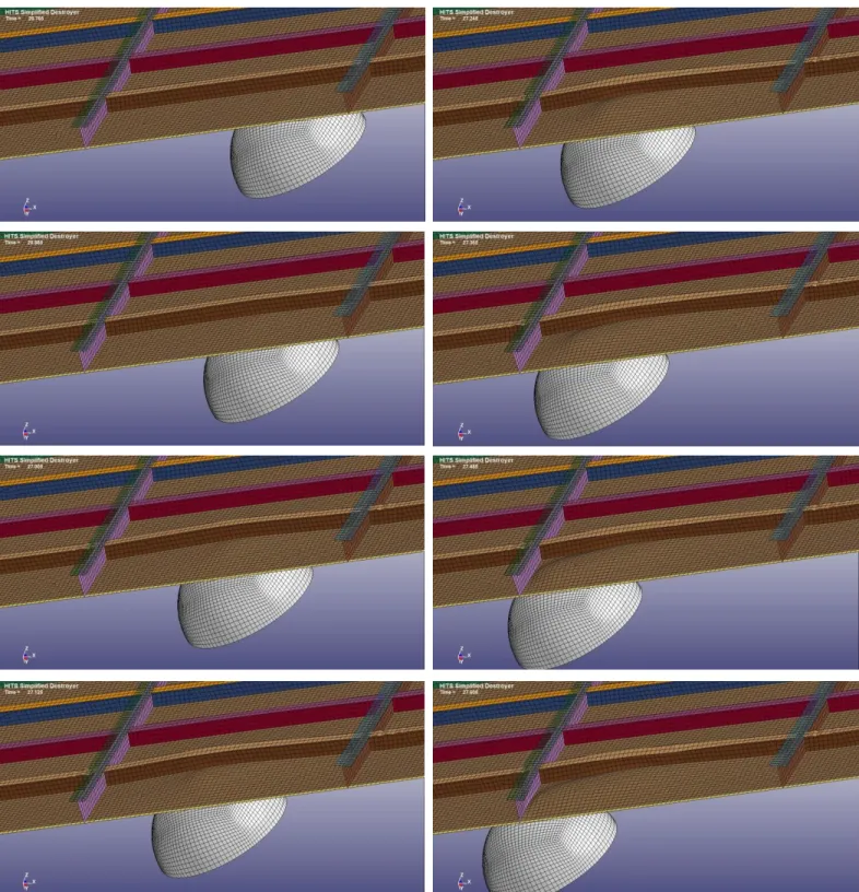
Figure 4 shows the force time series for the case of the 524 tonne ice mass initially impacting the grillage segment at a stiffener location and near a frame. The secondary ‘peak’ corresponds to the sliding ice-knob contacting the hull plating that was supported by a frame. The oscillationsin load at the top of the secondary peak correspond to elastic oscillations of the meshed hull segment due to the ice-knob impacting the frame. Further evidence (not shown here) of the elastic oscillations was observed in the normal-to-the-surface displacement of the hull at a particular location outside of the region of plastic damage. The resonant frequency is ~ 48 Hz. Figure 5 shows an image sequence from the simulation illustrating the progressive damage to the grillage structure during the sliding impact. The damage involves indentation of the plating, and bending/buckling of the stiffener and frame. Figure 6 shows the maximum deformable plate deflection associated with the impact. We note that the maximum load generated by the collision (~ 769 kN) was greater than the damaging load generated during the HITS simulation study conducted in 2017 where ice impacts occurred on a similar ship grillage. The load differences are associated with the generally larger impacted ice masses in the present study. As expected, some bow-wave induced surge and sway of the ice mass occurred prior to the impact (data not shown here).
Figure 7 shows the force time series for the case of the grillage segment impacting the 181 tonne ice mass. The maximum first-peak load value (~ 171 kN) induced significantly less plastic damage to the grillage than the larger ice-mass case. In contrast to Figure 5, that showed considerable plastic damage, relatively little damage was evident on the hull segment for the 181 tonne ice mass impact at the time of first-peak load. The sliding impact caused a wide-area shallow dent of ~ 11 mm depth, whereas the former heavier impact created a dent with a depth of ~ 59 mm.
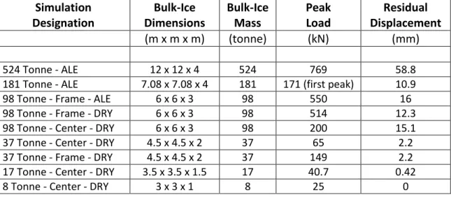
Towards the end of this study we wished to determine what the size of an ice mass would be that caused no damage at all to the vessel. Consequently, a wet-case simulation was run using a smaller ice mass of 98 tonnes. This also showed some grillage damage. So additional simulations were conducted using progressively smaller ice masses until no damage was produced. The results for the additional cases, where the impacts for most occurred roughly at the midpoint between two vertical frames, are shown in Table 4 and Figures 8 and 9, along with the results from the former heavier ice mass cases. Note that due to time constraints most of these simulations were run in ‘dry’ conditions, that is, hydrodynamics associated with water were not included since these simulations took far less time to run than ‘wet’ ALE simulations (1 hour versus more than 25 hours). However, we did conduct two simulations (one ‘wet’ and one ‘dry’) using the 98 tonne ice mass, where the impact initiated at a frame, to confirm that the impact loads were in reasonable agreement (see Table 4).
The results in Table 4 and Figures 8 and 9 are illuminating. They indicate that some level of damage, albeit diminishingly small, occurred as the ice masses and associated peak loads get smaller until eventually an ice mass of 8 tonnes produced no damage at all, where the peak load was 25 kN. Not surprisingly, this ice mass is less than the hybrid structure/ice mass used in the study by Gagnon and Quinton (2017) where grillage damage was evident. Also noteworthy is that the data indicate a fairly linear trend in the degree of damage associated with peak loads and ice masses. Note that in these results we are using ‘residual displacement’, the maximum non-recoverable indentation of the hull plating, as an index of ‘damage’. Using the fit equation in Figure 8, and the peak load value (260 kN) from Gagnon and Quinton (2017) for an ice impact on a similar grillage, we obtain a residual displacement of 18.4 mm, where those authors reported a value of 24 mm. These values corroborate when one considers that the similar
5
grillages did have some structural differences, and in the present case the impacts were nearer to a stiffener than in the former case (leading to less displacement).
There have been many numerical simulation studies of ship interactions with ice. An extensive review has been provided by Xue et al. (2020). Much of the work has related to ship performance in broken ice and through ice sheets. Due to the particular focus of most of the studies, damage to the vessel was not considered and hydrodynamic aspects were treated in a simplified manner, or not included. The first ship-ice collision simulation to include damage to the vessel and full hydrodynamics was by Gagnon and Wang (2012), using a validated ice model.
A somewhat similar study to the present one, involving simulations of a ship collision with a bergy bit, has been conducted by Liu et al., 2011. It is difficult to compare our results with those results because the scenarios in both studies are very different. The grillage in the other study had a different configuration and was much stronger than the present case. Furthermore, that work did not incorporate water (i.e. hydrodynamics), while some of ours did, so the ice mass was not a free floating object and its velocity against the vessel was fixed. Also the collision was not a sliding load scenario. Perhaps the most important difference was the ice model used that had mesh elements that eroded in response to a critical stress. That led to the formation of gaps in places in the ice contact zone where elements disappeared. That may explain why the simulation did not appear to reflect the structure of the grillage in the pressure distribution patterns it produced. On the other hand, the damage to the grillage had some similarities with the present results, and those of Gagnon and Wang (2012), such as the apparent bending and buckling of structural members behind the plating.
For the case of the 524 tonne ice mass we performed further analysis to determine the average pressure and ice contact area as the impact progressed. Table 5 shows the contact area, average pressure and peak pressure at seven equally-spaced instances in time for a time span similar to that spanning the second to the seventh images in Figure 5. The average pressure was obtained by first determining what the contact area was, following the method of Gagnon and Wang (2012). This was done by viewing the grillage at specific instants in time where at each instant the interface pressure was shown for the grillage elements. By choosing an appropriate scale for the colored pressure display, in our case using the range 0.001–2 MPa, the contact area could be obtained by summing the individual areas of all elements showing any indication of interface pressure. The average pressure was determined for the set of elements that were in contact with ice at that particular instant in time by dividing the total force on the grillage by the contact area. Excluding the first and last data points, that correspond to the onset of plate contact and the collision with a supporting frame, the pressure is fairly constant (6.6 MPa), as was that of Gagnon and Wang (2012) at a value of ~ 3.8 MPa. The difference in the two pressure values is due to the fact that the load and contact area were much greater in the earlier work, even though the grillage segments were similar. This meant that in the former study the contact area fairly evenly spanned the plating in both unsupported areas and areas where there were stiffeners/frames, resulting in a representative average pressure. However, in the present case the loads and contact areas are much lower and consequently the contact zone does not span multiple stiffened and unstiffened regions of the plate. Hence, if the contact happens to occur in the proximity of a frame/stiffener, as was the case depicted in Figure 5, where the contact is at the location of a horizontal stiffener and is also in close proximity to a frame that it eventually collides with, the average pressure will consequently be higher. This point is further illustrated by the observation that both the average and peak pressures decrease between rows 3 and 6 in Table 5. This is due to the downward movement (on the impacted hull segment) of the contact
6
area away from the horizontal stiffener as the ice rotates slightly downwards on the damaged sloping plating during the course of the sliding impact. This is discernible in Figure 5, but more clearly visible in other graphics that could not be included here due to paper-length limitations. Another aspect of the pressure results from the simulation is the impressive degree of agreement with results of large double pendulum ice impact tests (Gagnon et al., 2020). These lab experiments involved fairly large (1 m base diameter) conically-shaped ice samples impacting a hard surface that was covered with high spatial and temporal resolution pressure-sensing technology. The highest loads from the impact tests (416-622 kN) were in approximately the same range of the load for the 524 tonne ice mass impact after the onset of contact (303-656 kN). The average pressure from the tests was about 7.4 MPa that compares reasonably well with 6.6 MPa from the simulation. The average hard-zone pressures from the tests were very consistent (~ 21.5 MPa), and compare with the peak pressures of the simulation (~ 20.4 MPa) quite well. One may ask how a ‘peak’ pressure value can match an ‘average’ hard-zone pressure. We conclude that this is due to the size of a unit pressure sensor (≤ 3 cm2) on the impact apparatus compared to the larger typical element size of the impacted hull segment in the simulation (~ 12 cm2). The unit pressure sensor is small enough to resolve pressure distribution within a given hard-zone region, that may range from 15 MPa to 52 MPa (Gagnon et al., 2020), whereas the much larger size of an element in the simulation gives a pressure value more representative of the average pressure of hard zones. Recall that actual peak local interface pressures during ice crushing in the brittle regime almost invariably are associated with regions of hard-zone contact, where the ice is relatively intact and the pressure is high, as opposed to soft-zone regions consisting of crushed ice (shattered spall debris) where local pressure is low (Gagnon, 1999).
3. Conclusions
The simulation results indicated that some level of damage, albeit diminishingly small, occurred (in a linear trend) as the ice masses and associated peak loads get smaller until eventually an ice mass of 8 tonnes produced no damage at all, where the peak load was 25 kN. The next ice-mass size up from that was 17 tonnes, that did produce a tiny amount of damage during a simulation. The simulations show the effect of where the ice impact occurs with respect to supporting stiffeners and frames behind the plating and how this can influence the peak loads and pressures that occur, and the extent of local damage.
Impressive agreement of average and hard-zone pressures from the 524 tonne ice mass collision simulation with those from large-scale ice impact lab tests on a rigid surface was noted. While this may bolster confidence in the ice model that was used in the simulation, the fact that the grillage plating was deforming during the collision in the simulation, whereas the lab impact tests were on a flat rigid surface, suggests the need for further study of impacts on rigid and deformable surfaces (e.g. ship grillages).
Acknowledgements
The authors are grateful to NRC and DRDC for their support of this work.
References
Gagnon, R.E., 1999. Consistent Observations of Ice Crushing in Laboratory Tests and Field Experiments Covering Three Orders of Magnitude in Scale. Proceedings of the 15th International Conference on Port and Ocean Engineering under Arctic Conditions, 1999, POAC-99, Helsinki, Finland, Vol. 2, 858-869.
7
Gagnon, R.E. and Derradji-Aouat, A., 2006. First Results of Numerical Simulations of Bergy Bit Collisions with the CCGS Terry Fox Icebreaker. Proceedings of IAHR, Sapporo, Japan, Vol. 2, 9-16.
Gagnon, R.E. and Wang, J., 2012. Numerical Simulations of a Tanker Collision with a Bergy Bit Incorporating Hydrodynamics, a Validated Ice Model and Damage to the Vessel. Cold Regions Science and Technology 81, 26-35.
Gagnon, R. and Quinton, B., 2017. Heavy Impact Test Site (HITS) Simulations. OCRE Report OCRE-TR-2017-012, Protected A.
Gagnon, R., Andrade, S.L., Quinton, B., Daley, C., and Colbourne, B., 2020. Pressure distribution data from large double-pendulum ice impact tests. Cold Regions Science and Technology 175 (2020) 103033.
Liu, Z., Amdahl, J., and Løset, S., 2011. Integrated numerical analysis of an iceberg collision with a foreship structure. Marine Structures 24 (4), 377–395.
Pearson, D. and Abbott, M., 2016. Notional Vessel Design Improvement. Contract Report DRDC-RDDC-2017-C100.
Xue, Y., Liu, R., Li, Z., and Han, D., 2020.A review for numerical simulation methods of ship– ice interaction. Ocean Engineering 215 (2020) 107853.
Figures and Tables
Figure 2. Notional Destroyer body plan. (From Pearson and Abbott (2016))
Figure 2. Notional Destroyer body plan. (From Pearson and Abbott (2016))
Figure 1. The full meshed volume used in the simulations: half-ship (red); air (green); water (blue); bulk-ice mass (yellow). The portion of the vessel hull that was given a high mesh density and deformable properties during ice impacts is visible. Note that the ice-knob (discussed below) is at the far corner of the bulk-ice mass and is not visible in this image.
Figure 5. The full meshed volume used in the simulations: half-ship (red); air (green); water (blue); bulk ice mass (yellow). The portion of the vessel hull that was given a high mesh density and deformable properties during ice impacts is visible. Note that the ice knob is at the far corner of the bulk ice mass and is not visible in this image.
8 Primary Structure Thickness (mm) Material
Shell Plate 8.5 DH36 Steel*
Frame 10.0 DH36 Steel
Frame Flange 8.0 DH36 Steel
Longitudinal Stiffener 5.0 DH36 Steel Longitudinal Flange 6.0 DH36 Steel
Ice Mass Name Shape/Dimensions Mass
(tonne)
Element Property During Impacts
Ice-knob (attached to all bulk-ice masses)
Hemisphere (1 m diameter) 0.24 Deformable
Medium Bulk-Ice Block Brick (7.1 m x 7.1 m x 4 m) 181 Rigid
Large Bulk-Ice Block Brick (12 m x 12 m x 4 m) 524 Rigid
Loa 150.5 m Lwl 142.6 m B 18.9 m Bwl 16.9 m T 6.7 m H (to 1 Deck) 14.0 m Displacement 7600.0 tonne Cruising Speed 18.0 kt Sprint Speed 28.0 kt Max Speed 29.0 kt
Figure 3. (Left) Bulk-ice mass with ice-knob attached at a corner. (Right) An expanded view of the ice-knob showing its refined mesh that suites the mesh size of the target hull segment (Figure 1).
*350 MPa yield strength; based on Gagnon and Quinton (2017) the Young’s Modulus is 200 GPa and the Tangent Modulus is 1.04 GPa
*350 MPa yield strength; based on the 2017 study the Young’s Modulus is 200 GPa and the Tangent Modulus is 1.04 GPa
Table 3. Characteristics of the ice-knob and the initial bulk-ice masses.
Table 3. Characteristics of the ice-knob and the initial bulk ice masses.
Table 2. NSR Primary shell scantling dimensions Frame 18 – 11. (From Pearson and Abbott (2016))
Table 2. NSR Primary shell scantling dimensions Frame 18 – 11. (From Pearson and Abbott (2016))
Table 1. Notional Destroyer principal particulars. (From Pearson and Abbott (2016)) Loa 150.5 m Lwl 142.6 m B 18.9 m Bwl 16.9 m T 6.7 m H (to 1 Deck) 14.0 m Displacement 7600.0 tonne Cruising Speed 18.0 kt Sprint Speed 28.0 kt Max Speed 29.0 kt
Table 1. Notional Destroyer principal particulars. (From Pearson and Abbott (2016))
Figure 4. Load time series for the simulated impact with the 524 tonne ice mass. The secondary ‘peak’ corresponds to the ice-knob contacting the hull plating that was supported by a frame. The oscillations in load at the top of the secondary peak correspond to elastic oscillations of the meshed hull segment due to the sliding ice-knob impacting the frame.
Figure 6. Load time series for the simulated impact with the 524 tonne ice mass. The secondary ‘peak’ corresponds to the ice-knob contacting the hull plating that was supported by a frame. The oscillations in load at the top of the secondary peak correspond to elastic oscillations of the meshed hull segment due to the ice-knob impacting the frame.
0 200 400 600 800 1,000 26.5 27.0 27.5 28.0 Imp act Lo ad (kN ) Time (s)
9
Figure 5. Sequence of images (top left to bottom right) from the simulation illustrating the progressive plastic damage to the grillage that developed during the sliding impact. The impact occurred on the lower portion of the meshed deformable segment of the vessel hull. The bottom edge of the hull segment is attached to a deck on the actual vessel and is therefore treated as a rigid boundary. As the ice-knob (white object) progresses to the left, and somewhat downwards, bending and buckling of the lowest horizontal stiffener and flange is evident. Crumpling of the flange on the stiffener is evident on the outsides of the two vertical frames where there is substantial compression of the flange due to the two vertical frames ‘leaning away’ from the prominent upward bending of the stiffener. Similarly, when the ice-knob reaches the vertical frame at the left, bending and buckling of the frame occurs. The flanges on the two vertical frames were given transparent characteristics to facilitate viewing of the local deformations. Time stamps are included on the images, where the real-time interval between successive images is 0.12 s.
10 Simulation Designation Bulk-Ice Dimensions Bulk-Ice Mass Peak Load Residual Displacement (m x m x m) (tonne) (kN) (mm) 524 Tonne - ALE 12 x 12 x 4 524 769 58.8
181 Tonne - ALE 7.08 x 7.08 x 4 181 171 (first peak) 10.9
98 Tonne - Frame - ALE 6 x 6 x 3 98 550 16
98 Tonne - Frame - DRY 6 x 6 x 3 98 514 12.3
98 Tonne - Center - DRY 6 x 6 x 3 98 200 15.1
37 Tonne - Center - DRY 4.5 x 4.5 x 2 37 65 2.2
37 Tonne - Frame - DRY 4.5 x 4.5 x 2 37 149 2.2
17 Tonne - Center - DRY 3.5 x 3.5 x 1.5 17 40.7 0.42
8 Tonne - Center - DRY 3 x 3 x 1 8 25 0
Table 4. Simulations summary: ice dimensions/mass; peak load; hull residual indentation depth.
Table 4. Simulations summary: ice dimensions/mass; peak load; hull residual indentation depth.
0.0 10.0 20.0 30.0 40.0 50.0 60.0 70.0 26.5 27.0 27.5 28.0 M axi m u m Pla ti n g In d en ta ti on (m m ) Time (s)
Figure 6. Maximum plating indentation time series for the simulated impact with the 524 tonne ice mass. The secondary ‘peak’ corresponds to the ice-knob sliding onto hull plating that was partially supported by a frame. The small oscillations in displacement at the top of the secondary peak correspond to resonant elastic oscillations of the meshed hull segment due to the ice-knob impacting the frame.
Figure 11. Maximum plating indentation time series for the simulated impact with the 524 tonne ice mass. The secondary ‘peak’ corresponds to the ice-knob sliding onto hull plating that was partially supported by a frame. The small oscillations in displacement at the top of the secondary peak correspond to resonant elastic oscillations of the meshed hull segment due to the ice-knob impacting the frame.
Figure 7. Load time series for the simulated ship impact with the 181 tonne ice mass. The initial impact peak at ~ 30.2 s is followed by a trough at ~ 30.5 s that corresponds to the ice mass bouncing off of, and almost losing contact with, the hull
segment during the sliding collision.
Hydrodynamic forces prevent the ice from fully rebounding away from the hull at the load trough and consequently load rises again towards a secondary peak as the ship and hull segment continue to move forward against the ice mass, as the ice-knob approaches a frame.
Figure 12. Load time series for the simulated ship impact with the 181 tonne ice mass. The initial impact peak at ~ 30. 2 s is followed by a trough at ~ 30.5 s that corresponds to the ice-knob and bulk-ice mass bouncing off of, and almost losing contact with, the hull segment during the sliding collision. Hydrodynamic forces prevent the ice from fully rebounding away from the hull at the load trough and consequently load rapidly rises again towards a secondary peak as the ship and hull segment continue to move forward against the ice mass.
11
Table 5. Contact Area, Load and Pressure Data for the 524 Tonne Ice Mass Simulation.
Table 3. Characteristics of the ice-knob and the initial bulk ice masses.
Time (s) Number of Elements Contact Area (sq. cm) Load (kN) Average Pressure (MPa) Peak Pressure (MPa) 26.81 20 244.5 79.1 3.23 9.89 26.94 41 493.6 303.2 6.14 21.53 27.07 52 636.3 502.9 7.90 27.25 27.20 72 881.5 579.8 6.58 22.67 27.34 70 845.2 533.2 6.31 17.81 27.47 71 861.9 502.0 5.82 12.84 27.60 28 337.4 656.3 19.45 42.68
Averages (red data) 61.2 743.7 484.2 6.55 20.42
Figure 9. Residual displacement versus ice mass for simulations covering a wide range of ice masses. Red-circle data points correspond to ‘wet-case’ ALE simulations, whereas the blue-circle data points relate to ‘dry-case’ simulations that did not include hydrodynamics. For all of the ‘dry’ simulations the ice impacts occurred between two vertical frames. Note that ‘residual displacement’ refers to the maximum non-recoverable indentation of the hull plating.
Figure 16. Residual displacement versus ice mass for simulations covering a wide range of ice masses. Red-circle data points correspond to ‘wet-case’ ALE simulations, whereas the blue-circle data points relate to ‘dry-case’ simulations that did not include hydrodynamics. For all of the ‘dry’ simulations the ice impacts occurred between two vertical frames. Note that ‘residual displacement’ refers to the maximum non-recoverable indentation of the hull plating.
Figure 8. Residual displacement versus peak load for simulations covering a wide range of peak loads. Red-circle data points correspond to ‘wet-case’ ALE simulations, whereas the blue-circle data points relate to ‘dry-case’ simulations that did not include hydrodynamics. For all of the ‘dry’ simulations the ice impacts occurred between two vertical frames. Note that ‘residual displacement’ refers to the maximum non-recoverable indentation of the hull plating.
Figure 15. Residual displacement versus peak load for simulations covering a wide range of peak loads. Red-circle data points correspond to ‘wet-case’ ALE simulations, whereas the blue-circle data points relate to ‘dry-case’ simulations that did not include hydrodynamics. For all of the ‘dry’ simulations the ice impacts occurred between two vertical frames. Note that ‘residual displacement’ refers to the maximum non-recoverable indentation of the hull plating.