Adaptive sampling and forecasting with mobile sensor networks

Adaptive Sampling and Forecasting

L .

With Mobile Sensor Networks

LIBRA

by

ARCHIVES

Han-Lim Choi

B.S., Korea Advanced Institute of Science and Technology (2000)

M.S., Korea Advanced Institute of Science and Technology (2002)

Submitted to the Department of Aeronautics and Astronautics

in partial fulfillment of the requirements for the degree of

Doctor of Philosophy

at the

MASSACHUSETTS INSTITUTE OF TECHNOLOGY

February 2009

@

Massachusetts Institute of Technology 2009. All rights reserved.

Author ...

...

Department of Aeronautics and Astronautics

September 30, 2008

C ertified by ...

Jonathan P. How

Professor of Aeronautics and Astronautics

Thesis Supervisor

Certified by ...

Nicholas Roy

Aista

Profesronautics and Astronautics

Certified by...

S/

James A. Hansen

Lead Scientist, Naval Research Laboratory

Certified by...

-

Emilio Frazzoli

Associate Professor

eronautiie and As rnautics

Accepted by ...

DavX4d[ Darmofal

Chairman, Department Committee on Graduate Students

Adaptive Sampling and Forecasting

With Mobile Sensor Networks

by

Han-Lim Choi

Submitted to the Department of Aeronautics and Astronautics on September 30, 2008, in partial fulfillment of the

requirements for the degree of Doctor of Philosophy

Abstract

This thesis addresses planning of mobile sensor networks to extract the best infor-mation possible out of the environment to improve the (ensemble) forecast at some verification region in the future. To define the information reward associated with sensing paths, the mutual information is adopted to represent the influence of the measurement actions on the reduction of the uncertainty in the verification variables. The sensor networks planning problems are posed in both discrete and continuous time/space, each of which represents a different level of abstraction of the decision space.

In the discrete setting, the targeting problem is formulated to determine the se-quence of information-rich waypoints for mobile sensors. A backward formulation is developed to efficiently quantify the information rewards in this combinatorial deci-sion process. This approach computes the reward of each possible sensing choice by propagating the information backwards from the verification time/space to the search space/time. It is shown that this backward method provides an equivalent solution to a standard forward approach, while only requiring the calculation of a single co-variance update. This work proves that the backward approach works significantly faster than the forward approach for the ensemble-based representation.

In the continuous setting, the motion planning problem that finds the best steer-ing commands of the sensor platforms is posed. The main difficulty in this continuous decision lies in the quantification the mutual information between the future verifica-tion variables and a continuous history of the measurement. This work proposes the

smoother form of the mutual information inspired by the conditional independence

relations, and demonstrates its advantages over a simple extension of the state-of-the-art: (a) it does not require integration of differential equations for long time intervals, (b) it allows for the calculation of accumulated information on-the-fly, and (c) it provides a legitimate information potential field combined with spatial interpo-lation techniques.

The primary benefits of the presented methods are confirmed with numerical experiments using the Lorenz-2003 idealistic chaos model.

Thesis Supervisor: Jonathan P. How

Acknowledgments

First of all, I would like to thank my advisor Prof. Jonathan How for letting me to explore this interesting research and for being a model of a good/hard-working advisor himself. I am thankful to Prof. Nicholas Roy for the series of informative comments and inputs he has provided in the biweekly DDDAS meetings. I appreciate Dr. Jim Hansen for guiding me to the weather world and explaining me all the jargons I was unfamiliar with. Many thanks to Prof. Emilio Frazzoli for insightful comments that helped me set a firm standpoint to the big picture of my work. I also thank my thesis readers, Prof. Karen Willcox and Prof. Hamsa Balakrishnan, for providing me good sources of inputs to improve the presentation of the work in this thesis.

I would like to thank my former advisor Prof. Min-Jea Tahk at KAIST for his invaluable advices on both research and a real life. I thank my former advisor at MIT, Prof. Eric Feron now in Georgia Tech, who helped me easily settle down at MIT. I appreciate Prof. Paul Barton in Chemical Engineering at MIT for his insightful inputs on the optimization work in the appendix of my thesis. I am grateful to Prof. Jean-Jacques Slotine for his help in my individual research on the nonlinear observer design.

Many of my fellow labmates in the Aerospace Controls Laboratory have been a good source of ideas; especially, I would like to thank Luca Bertuccelli and Emily Craparo for all the critical (cross-)readings and insightful comments on my papers. The help of Kathryn Fischer in organizing the trips (adapted to my preference) should be acknowledged.

I am grateful to my friends including Korean community in MIT Aero/Astro, KAISTians at MIT, and KSHS Class 12 in Korea. Especially, I would like to thank Sang-il Lee and Jaemyung Ahn who started MIT Aero/Astro lives at the same time, and the five best friends of mine, "Eagle Five."

I especially want to thank my family in Korea: my parents who have supported and believed in me for 30 years, my brother Yun-Lim who has been my best friend and a model of the active, my parents-in-law who already started calling me Dr. Choi three years ago and have provided endless support, my brother-in-law Changbum who has so believed in me, and my sister-in-laws Dajeong and Anna.

Most importantly, I would like to thank my wife Chorong, the source of every pleasure and happiness of mine. Without her unbelievable love, encouragement, and patience, I could not make it to this point - I love you. Finally, thanks our baby boy, Robin.

This research was funded by NSF CNS-0540331 as part of the DDDAS program. The author also gratefully acknowledges funding from the Samsung Scholarship.

Contents

1 Introduction

1.1 Information Rewards . ...

1.1.1 Discrete-Time Mutual Information [Chapter 3] . .

1.1.2 Continuous-Time Mutual Information [Chapter 5] 1.2 Path Planning . . . ...

1.2.1 Discrete Targeting [Chapter 4] . . . ..

1.2.2 Continuous Motion Planning [Chapter 5] . . . . 1.3 Implementation Issues . ...

1.3.1 Sensitivity Analysis of Targeting [Chapter 6] 1.4 Summary of Contributions ... ... 2 Preliminaries

2.1 Entropy and Mutual Information ... 2.2 Ensemble Square-Root Filter ... 2.3 Lorenz-2003 Chaos Model ...

3 Sensing Point Targeting

3.1 Sensor Selection Problems . ...

3.1.1 Ensemble-Based Adaptive Observation Targeting . . . . . 3.1.2 Sensor Management for EKF Tracking of a Moving Target 3.2 Computation Time Analysis . ...

3.2.1 Conventional Covariance Form ... . . . . . . ..

3.2.2 EnSRF-Based Targeting . . . . . . . . .. 3.3 Sequential Greedy Strategies . ... ...

3.3.1 Algorithms ... 3.3.2 Computation Time . ... 3.3.3 Summary of Computation Time Analysis ... 3.4 Numerical Results ... 17 .. . . . 20 . . . . . 20 . . . . . 21 .. . . . 23 .. . . . 23 . . . . . 23 .. . . . 24 . . . . . 24 .. . . . 24 27 27 30 32 35 36 39 42 45 45 50 54

3.4.1 Ensemble-Based Targeting for Weather Forecast ... 59

3.4.2 Sensor Selection for EKF Target Tracking . ... 62

3.4.3 Summary ... ... 65

3.5 Conclusions ... ... ... 66

4 Multi-Sensor Platform Targeting 67 4.1 Problem Formulation .... ... ... 68

4.2 Algorithm ... ... .. 70

4.2.1 Backward Selection ... ... ... 71

4.2.2 Reachable Search Space ... .. 71

4.2.3 Action Space Search ... .. . 74

4.2.4 Cut-Off Heuristics ... .. . . 75

4.2.5 Algorithm Summary ... .... 79

4.3 Decomposition Schemes ... ... 80

4.4 Numerical Simulations ... ... 82

4.4.1 Setup ... ... ... .. 82

4.4.2 Effect of Cut-Off Heuristics ... 83

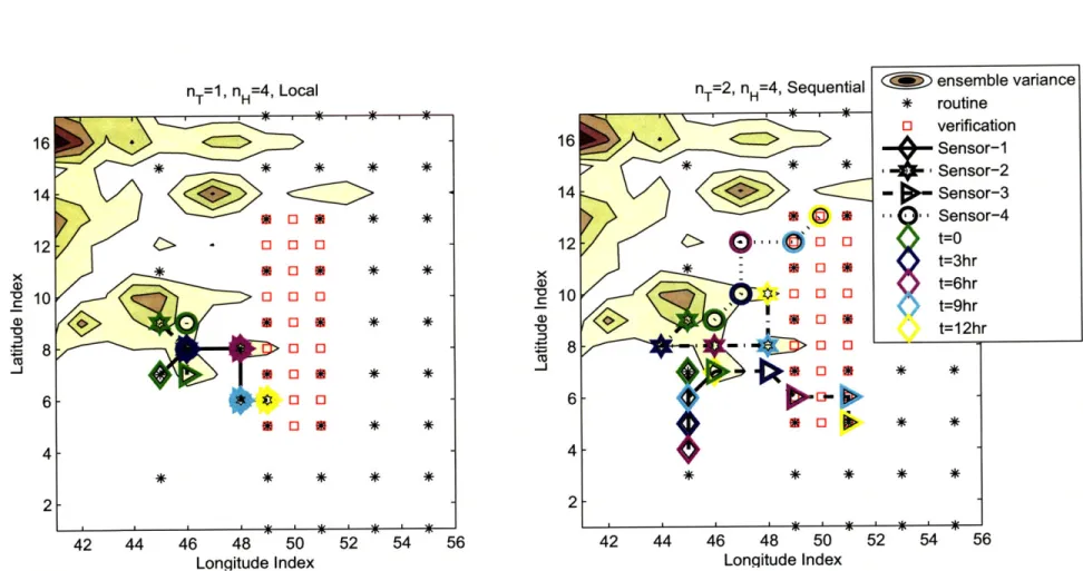
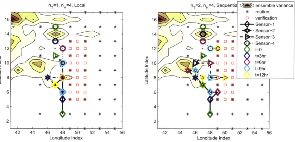
4.4.3 Comparison of Decomposition Schemes . ... 84

4.4.4 Effect of Routine Networks . ... .. 90

4.5 Conclusions ... ... .. 90

5 Continuous Sensor Motion Planning 91 5.1 Problem Description ... ... . 93

5.2 Information by Continuous Measurement . ... . 94

5.2.1 Linear System Model ... ... 94

5.2.2 Filter Form ... ... . 95

5.2.3 Smoother Form ... ... 98

5.2.4 On-the-fly Information and Mutual Information Rate ... 107

5.2.5 Smoother-Form On-the-fly Information for Forecasting (SOIF) 109 5.3 Path Representation ... ... 115

5.4 Path Planning Formulations ... .. . 118

5.4.1 Optimal Path Planning ... ... 118

5.4.2 Information Field and Real-Time Steering . ... 119

5.5 Numerical Simulations ... ... 120

5.5.1 Scenarios ... ... 120

5.5.2 Results ... ... .. 121

5.6.1 Backward Selection and Smoother Form . . . 5.7 Conclusions . . ...

6 Sensitivity Analysis for Ensemble-Based Targeting 6.1 Limited Ensemble Size ...

6.2 Effects of Limited Ensemble Size on Targeting . . . 6.2.1 Well-Posedness . ...

6.2.2 Numerical Studies ...

6.3 Analysis of Effects of Limited Ensemble Size . . . . 6.3.1 Sample Entropy Estimation . . . ... 6.3.2 Range-to-Noise Ratio . ...

6.3.3 Probability of Correct Decision . . . .

133 . . . . . . 133 . . . . . 135 . . . . . . 135 . . . . . . 137 . . . . . . . . 141 . . . . . . 141 . . . . . . 144 . . . . . . 147

6.3.4 Confirmation of Analysis with Lorenz-95 Targeting Example 6.4 Conclusions ... 7 Conclusions 7.1 Contributions . ... 7.2 Future Work ... ... A Analysis of Submodularity A.1 Conditions for Submodularity . .... A.2 Numerical Results with Sensing-Point Targeting . . . . B Extension of Smoother Form to Tracking Problems B.1 Smoother-Form On-the-fly Information for Tracking (SOIT) B.1.1 Information . . ... B.1.2 Information Rate . ... B.2 On-the-fly Information for Receding-Horizon Formulations B.3 Numerical Examples . . ... B.3.1 Tracking Interpretation of Example in Chapter 5 B.3.2 Sensor Scheduling . ... B.3.3 Target Localization ... 167 . . . . . 168 . . . . . 168 . . . . . 169 . . . . . 169 . . . . . 172 . . . . . 172 . . . . . 172 . . . . . 173

C An Outer-Approximation Algorithm for Maximum Entropy Sensor Selection 179 C.1 Introduction ... ... 179

C.2 Problem Formulation ... ... 182

C.2.1 Generalized Maximum Entropy Sampling ... . . . 182 126 132 151 152 153 153 155 157 157 164

C.2.2 Mixed-Integer Semidefinite Program Formulation ... . 183

C.3 Algorithm ... ... 185

C.3.1 Primal Problem ... ... 185

C.3.2 Relaxed Master Problem ... . 186

C.4 Numerical Experiments with MES ... . 187

C.5 Constrained Sensor Management Problem . ... 188

C.5.1 Problem Description ... .... 188

C.5.2 Modification of BB-NLP . ... .. 189

C.5.3 Numerical Results ... ... 190

C.6 Concluding Remarks ... ... 193

D More Numerical Results for Chapter 5 195

List of Figures

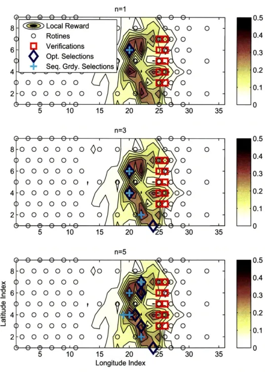
1-1 Adaptive sampling for weather forecast improvement . ... 19 3-1 Sensor targeting over space and time . ... . . 36 3-2 Observation structure over the search space and time ... 40 3-3 Targeted sensor locations determined by the optimal and the sequential

greedy methods ... ... . 60

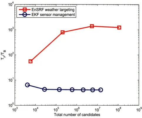
3-4 Optimal Sensor Selection for EKF Target Tracking . ... 64 3-5 Comparison of relative computational advantage of the backward

for-mulation ... ... ... 65

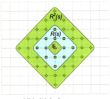
4-1 Multi-UAV targeting in the grid space-time . ... 68 4-2 Reachable zones by a single agent in two-dimensional grid space . . . 73 4-3 Schematics of team-based decomposition with two different

communi-cation topologies ... ... 80

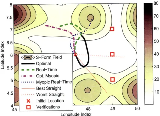
4-4 Targeting solutions for the sensors initially close to each other . . .. 87 4-5 Targeting solutions for the sensors initially dispersed widely .... . 88 5-1 Continuous motion planning of a sensor for best information forecast 93 5-2 On-the-fly information by a partial measurement path Zt ... 115 5-3 Sensor trajectories for Scenario 1 overlaid with the smoother form

in-formation potential field . ... ... 123 5-4 Sensor trajectories for Scenario 1 overlaid with the filter form

informa-tion potential field ... ... ... 123 5-5 Sensor trajectories for Scenario 2 overlaid with the smoother form

in-formation potential field ... ... 124 5-6 Sensor trajectories for Scenario 2 overlaid with the filter form

informa-tion potential field ... ... 124 5-7 Snapshots of the optimal trajectory with evolution of information field

5-8 Snapshots of the trajectory of real-time steering with evolution of

in-formation field (Scenario 1) ... .... 128

5-9 Snapshots of the best straight-line trajectory with evolution of infor-mation field (Scenario 1) ... ... 129

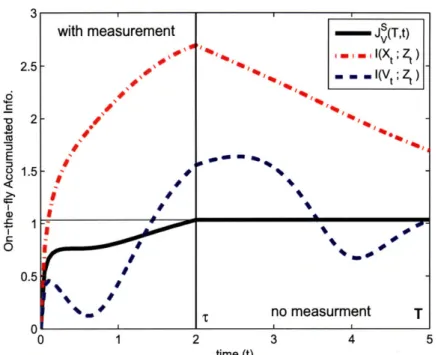
5-10 Time histories of information accumulation in Scenario 1 ... 130

5-11 Time histories of information accumulation in Scenario 2 ... 130

5-12 Graphical structure of the presented approaches . ... 131

6-1 Errorbar plots of predicted/actual optimal reward values ... 139

6-2 Errorbar plots of predicted/actual optimal objective values when using trace measure ... ... . 141

6-3 Probability density of estimation error (m = 99) . ... 143

6-4 Standard deviation of

f

6-5 Standard deviation of R~ - I ... ... . 145

6-6 Probability of Correct Decision for targeting with q candidates . . . . 150

6-7 Range-to-noise ratio for Lorenz-95 example for various m and n . . . 151

A-1 The maximum and minimum value of gap between the prior and the posterior mutual information . ... .. 165

B-i Switching sequences for OPT, F-RH, and S-R . ... 174

B-2 Smoother-form and Filter-form information accumulation for OPT, F-RH, and S-RH ... ... ... 174

B-3 Sensor trajectories for target localization . ... 176

B-4 Time histories of entropy of (a) target's x-position, (b) target's y-position, (c) overall position estimate . ... 176

B-5 Smoother-form and filter-form on-the-fly information values used for planning ... .... ... ... ... 177

C-1 An illustrative solution representing trade-off between information and communication (N = 40) . ... ... . 191

D-1 Snapshots of the optimal trajectory with evolution of information field (Scenario 1) ... ... . 196

D-2 Snapshots of the trajectory of real-time steering with evolution of in-formation field (Scenario 1) ... .... 197

D-3 Snapshots of the best straight-line trajectory with evolution of infor-mation field (Scenario 1) ... ... . 198

D-4 Snapshots of the worst straight-line trajectory with evolution of infor-mation field (Scenario 1) ... ... 199 D-5 Snapshots of the myopic optimal trajectory with evolution of

smoother-form insmoother-formation field (Scenario 1) . ... 200 D-6 Snapshots of the myopic optimal trajectory with evolution of filter-form

information field (Scenario 1) ... ... 201 D-7 Snapshots of the trajectory of myopic real-time steering with evolution

of smoother-form information field (Scenario 1) . ... 202 D-8 Snapshots of the trajectory of myopic real-time steering with evolution

of filter-form information field (Scenario 1) . ... 203 D-9 Snapshots of the optimal trajectory with evolution of information field

(Scenario 2) . . . . ... ... ... 204 D-10 Snapshots of the trajectory of real-time steering with evolution of

in-formation field (Scenario 2) ... ... 205 D-11 Snapshots of the best straight-line trajectory with evolution of

infor-mation field (Scenario 2) ... ... 206 D-12 Snapshots of the worst straight-line trajectory with evolution of

infor-mation field (Scenario 2) . . ... ... ... 207 D-13 Snapshots of the myopic optimal trajectory with evolution of

smoother-form insmoother-formation field (Scenario 2) . ... 208 D-14 Snapshots of the myopic optimal trajectory with evolution of filter-form

information field (Scenario 2) ... ... 209 D-15 Snapshots of the trajectory of myopic real-time steering with evolution

of smoother-form information field (Scenario 2) . ... 210 D-16 Snapshots of the trajectory of myopic real-time steering with evolution

List of Tables

3.1 Summary of the asymptotic complexity for the cases where N >

max{M, n}, LE > max{M, n}, min{M, n} > 1 . ... 58 3.2 Summary of relative efficiency for the cases where N > max{M, n}, LE

max{M, n}, min{M, n > 1 .... ... ... 58 3.3 Mutual information values for the targeting solutions by different

tar-geting strategies (Backwards are all same as Forwards if both are

avail-able) ... ... ... 62

3.4 Solution time of exhaustive searches for ensemble targeting problems

with Lorenz-95 model ... ... 63

3.5 Solution time of sequential greedy strategies for ensemble targeting problems with Lorenz-95 model ... . . 63 3.6 Solution time for forward and backward methods for EKF sensor

man-agement (N = 30) ... ... 64

4.1 5-simulation average performance of the cut-off heuristics for different e 84

4.2 Initial Locations ... ... 85

4.3 Average value of I(Z*[t:tK]; V) for 4 sensors with dense configuration

(I(Zsnd[tl:tK]; V) = 6.5098) . ... ... 85 4.4 Average computation time (seconds) for 4-sensor problems ... 89 4.5 Average value of Z(ZS,[tl:tK]; V) for 4 sensors with dispersed

configura-tion ( I(Zsnd[tl:tK]; V) = 5.7066 ) ... .. ... .... 89 4.6 Average value of I(Z'[tl:tK]; V) for 4-sensor case with smaller routine

networks ( I(Zsrd[tl:tK]; V) = 1.8037 ) ... 89

5.1 Scenarios for continuous motion planning . ... . 121 5.2 Information rewards for different strategies . ... 122 C.1 Average Computation time (sec.) [# of UBD computations] .... . 188 C.2 Avg. Comp. time (sec.) [# of UBD computations] for SMP .... . 192

Chapter 1

Introduction

This thesis presents new algorithms for planning of mobile sensor networks to extract the best information out of the environment. The design objective of maximizing some information reward is addressed in both discrete and continuous time and space in order to represent different levels of abstraction in the decision space. The sensor

targeting problem that locates a sequence of information-rich waypoints for mobile

sensors is formulated in the discrete domain; the motion planning problem that deter-mines the best steering commands of the sensor platforms is posed in the continuous setup. Key technological aspects taken into account are: definition and effective quantification of the information reward, and design mechanism for vehicle paths considering the mobility constraints.

This work addresses the above planning problems in the context of adaptive

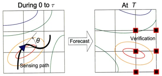
sam-pling for numerical weather prediction. The goal of adaptive samsam-pling is to determine

when and where to take supplementary measurements to improve the weather fore-cast in the specified verification region, given a fixed observation network (See Figure 1-1). The complex characteristics of the weather dynamics, such as being chaotic, un-certain, and of multiple time- and length-scales, requires the use of a large sensor net-work [1-5]. Expanding the static observation netnet-work is limited by geographic aspects; thus, an adaptive sensor network incorporating mobile sensor platforms (manned or possibly unmanned) has become an attractive solution to effectively construct larger networks.

The primary challenges in this adaptive sampling are:

* Spatial and temporal coupling of the impact of sensing on the uncertainty re-duction: Since a decision by one sensing agent affects the information reward for decisions by other sensing agents, the selection of the best set of measurements should take into account these coupling effects. Due to this type of coupling, the adaptive sampling problem is NP-hard [6, 7].

* Enormous size of systems: A typical state dimension of the weather system is 0(106) and a typical measurement dimension of the sensor networks is 9(103) [4]; therefore, the adaptive sampling is a very large-scale combinatorial decision making.

* Long forecast horizon: The quantity of interest in the adaptive sampling prob-lem is the weather variables over the verification region in the far future; thus, computation of the impact of sensing on the verification region typically incurs a computationally expensive forward (in time) inference procedure. Therefore, a solution method should feature an effective forward inference.

* Nonlinearity in dynamics: The weather system is highly nonlinear; therefore, incorporation of nonlinear estimation schemes are essential in adaptive sam-pling.

* Interest in a specified subset of the entire state space: The fact that the ver-ification region is a small subset of a large state space brings difficulty in the adoption of well-established techniques [6, 8-10] for the selection problems with submodular reward functions.

Previously, there were two representative types of adaptive sampling approaches: One approach locates the sites where a perturbation from them propagated through a linearized dynamics exhibits the largest growth of errors in the verification region [1-3]. This approach characterizes the direction of error growth embedded in the dy-namics, but cannot take into account specific details of the data assimilation scheme such as the uncertainty level of the state estimates. The other approach quantified

600

SO//V

40O

Figure 1-1: Adaptive sampling for weather forecast improvement: Paths for four UAV sensor platforms ( cyan

*,

0)

(red 0) in 3 days.

the variation in the future forecast error based on an ensemble approximation of the extended Kalman filter [4, 5], and sought for the sensing points that reduce the trace of the covariance matrix of the future verification variables. This type of approach can incorporate the uncertainty information into the sampling decision. However, due to the challenges listed above, only simple selection strategy has been tractable. For instance, two flight paths were greedily selected out of 49 predetermined paths in [4].

This thesis addresses these challenges by considering two levels of decision making - the targeting problem and the motion planning problem. The targeting problem posed in the discrete time/space domain concerns a longer time- and length-scale decision for sensor platforms where the nonlinear weather dynamics is represented

contin-uous time/space domain deals with a shorter time- and length-scale decision when the linear system approximates a short-term local behavior of the original nonlinear dynamics. This hierarchical approach enables better incorporation of the multi-scale aspect of the weather system with providing better computational efficiency. More-over, this work takes an information-theoretic standpoint to define and quantify the impact of a measurement on the uncertainty reduction of the verification variables, taking advantage of some important properties of the mutual information that facil-itate computationally efficient decision making.

1.1

Information Rewards

1.1.1

Discrete-Time Mutual Information [Chapter 3]

The notion of mutual information has been frequently [6, 8-14] used to define the information reward for discrete selection, since it represents the degree of depen-dency between the sensor selection and the quantity of interest. For the problems of tracking (moving) targets, the mutual information between the target states and the measurement sequence has been used to represent the improvement of the estimation performance by the measurement selection [10, 12-14]. In addition, in [6, 8, 9, 11], mutual information was used to quantify the uncertainty reduction of the temperature field over the unobserved region by the sensor selection. Since the use of mutual in-formation usually incurs substantial computational cost, all the algorithms have been developed in ways that either approximate the mutual information using other simple heuristics [12] or introduce some greediness in the selection decision [6, 8-11, 14].

Relevant approaches to finding the globally optimal solution to a mathematically equivalent problem to sensor selection were addressed in the context of environmen-tal monitoring. Anstreicher et al. [15] presented a 0-1 nonlinear program called a maximum-entropy remote sampling problem and proposed a branch-and-bound al-gorithm to solve this problem with global optimality. Although the authors of that paper did not employ the same terminology, they used linear algebraic properties to

derive a formulation that is equivalent to the sensor selection based on commuta-tivity of mutual information. But the problem sizes considered in [15] were much smaller than the ones usually encountered in a targeting problem in a large-scale sen-sor network. The observation that the global optimal solutions to the sensen-sor selection decisions have been available only for small-size problems points out the importance of effective computation of the information reward in designing a large-scale sensor network.

This thesis provides an efficient way of quantifying the mutual information to be used for a large-scale sensor targeting problem. Mutual information is used as a mea-sure of uncertainty reduction and it is computed from the ensemble approximation of the covariance matrices. The commutativity of mutual information is exploited to address the computational challenge resulting from the expense of determining the impact of each measurement choice on the uncertainty reduction in the verifica-tion site. This enables the contribuverifica-tion of each measurement choice to be computed by propagating information backwards from the verification space/time to the search space/time. This backward computation is shown to significantly reduce the required number of ensemble updates, which is a computationally intensive part of the adap-tive planning process, and therefore leads to much faster decision making. In this thesis, theoretical computation time analysis proves the computational benefit of the backward approach, which is also verified by numerical simulations using an idealized weather model.

1.1.2

Continuous-Time Mutual Information [Chapter 5]

Although mutual information in the continuous-time domain does not appear to be as well-known in the robotics and sensor networks communities, in the information theory context, there has been a long history of research about the mutual informa-tion between the signal and observainforma-tion in the continuous-time domain. Duncan [16] showed that the mutual information between the signal history and observation his-tory (i.e. signal during [0, t] and observation during [0, t]) is expressed as a function of estimation error for a Gaussian signal through an additive Gaussian channel. Similar

quantification is performed for non-Gaussian signal [17, 18] and fractional Gaussian channel [19]. On the other hand, Tomita et al. [20] showed that the optimal filter for a linear system that maximizes the mutual information between the observation history for [0, t] and the state value at t is the Kalman-Bucy filter; Mayer-Wolf and Zakai [21] related this mutual information to the Fisher information matrix.

Recently, Mitter and Newton [22] presented an expression for the mutual infor-mation between the signal path during [s, t], s < t and the observation history, with statistical mechanical interpretation of this expression. Newton [23, 24] extended his previous results by quantifying the mutual information between the future signal path during [t, T], t < T and the past measurement history during [0, t] for linear time-varying [23] and nonlinear [24] systems. However, it should be noted that all these previous quantifications have been about the state and observation. On the contrary, this study deals with the mutual information between the values of a subset

of the state at T and the observation history during [0, t] when T > t.

As an effective mechanism to quantify the mutual information for forecast prob-lems, this thesis proposes the smoother form, which regards forecasting as fixed-interval smoothing. Based on conditional independence of the measurement history and the future verification variables for a given present state value, the smoother form is proven to be equivalent to the filter form that can be derived as a simple extension of previous work [20-22]. In contrast to the filter form, the smoother form can avoid integration of matrix differential equations for long time intervals, resulting in better computational efficiency. Moreover, since the smoother form pre-processes the effect of the verification variables and the future process noise, the information accumu-lated along the path and the rate of information accumulation can be computed on the fly with representing the pure impact of sensing on the uncertainty reduction. This facilitates more adaptive planning based on some information potential field.

1.2

Path Planning

1.2.1

Discrete Targeting [Chapter 4]

Discrete path planning of sensor platforms is based on the abstraction of a measure-ment path as a sequence of waypoints [14, 25-27]. Then, the information reward gathered along a path is represented by the mutual information between a finite number of sensing points distributed over time and a finite number of future verifica-tion variables. While the backward formulaverifica-tion enables computaverifica-tion of this mutual information value, the primary question in the discrete path planning is how to incor-porate the constrained vehicle motions in an effective manner, and how to maintain computational tractability and the performance level in large-scale decisions.

In this thesis, the aspect of the vehicle mobility constraint is dealt with by using the concept of the reachable search space and the action space search. These two allow for reduction of the search space dimension by excluding inadmissible solution can-didates. Also, a cut-off heuristics utilizing a simplistic approximation of the mutual information provides further computational efficiency.

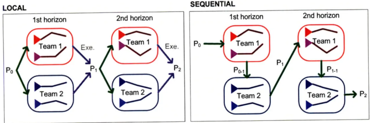
To handle computational burden in the optimal targeting of multiple sensing plat-forms, decomposition schemes that break down a large-scale targeting problem into a series of smaller problems are presented. The comparative study of different de-composition topologies indicates the crucialness of the coordinated modification of covariance information to achieve good overall team performance.

1.2.2

Continuous Motion Planning [Chapter 5]

The spatially continuous feature of the vehicle path can be addressed by using spatial interpolation techniques such as Kriging [28] and Gaussian Processes Regression [29] that predict a value of the quantity of interest at an arbitrary point in continuous space as a function of values at a finite number of grid points. Using this technique, the measurement action along a continuous path can be modeled as evolution of the observation function - the observation matrix in a linear system, which appears in

the integrand of the matrix differential equation for the smoother-form information reward. Thus, continuous variation of the vehicle location will change the integrand of the matrix differential equation through the observation matrix, and this ultimately leads to the change in the information reward value.

Utilizing this representation of continuous paths, many standard path planning methods are explored. The optimal path planning and a real-time gradient-ascent steering based on information potential fields are presented.

1.3

Implementation Issues

1.3.1

Sensitivity Analysis of Targeting [Chapter 6]

In real weather prediction systems, due to the computational expense of integrating forward a large-scale nonlinear system, and storing large ensemble data sets, the en-semble size that can be used for adaptive sampling is very limited [30-32]. In spite of limitation of ensemble diversity in real weather prediction systems, there have been little studies on the sensitivity of the ensemble-based adaptive sampling to the ensem-ble size. As an essential step toward real implementation of the presented targeting mechanism, this thesis performs a sensitivity analysis from both experimental and theoretical points of view. Monte-Carlo experiments characterize important sensi-tivity properties anticipated with small ensemble size, and analytical formulas that relate the ensemble size and the expected performance variation are derived based on the statistics theory for sample entropy estimation.

1.4

Summary of Contributions

* Discrete-Time Mutual Information A similar backward formulation based

on commutativity of mutual information was first presented in [15] in the process of formulating a 0-1 program, and previous work [10, 14] dealing with the task of tracking a moving target recognized the convenience and efficiency it gives in representing and calculating the associated covariance information. However, a

key contribution of this thesis is to clearly show the computational advantages of the backward form caused by the reduction of the number of covariance updates, by expanding the benefits in [10] to much more general sensor selec-tion problems. In addiselec-tion, with two key examples, this thesis shows that the backward selection performs never slower than the forward selection and also clearly identifies the types of systems for which the backward offers a substantial computational improvement over the forward. This newly-identified advantage of the backward selection, which is amplified for large-scale decisions, was not addressed in previous work [10, 14], and is a unique contributions of this thesis.

* Continuous-Time Mutual Information Despite well-established theory on

mutual information between the states and observations in the continuous-time domain, it is a unique and novel contribution of this thesis to derive the expres-sions for the forecast problem. In particular, the smoother form is proposed to well account for distinctive characteristics of forecasting, i.e., interest in a particular subset of the states in the far future. Also, this work clearly identifies the advantages of the smoother form over the filter form in the aspects of com-putational efficiency, robustness to modeling errors, and concurrent knowledge of information accumulation.

* Multi-Sensor Platform Targeting On the backbone of the backward se-lection formulation, this work presents the overall algorithmic procedure for multi-sensor platform targeting. In the process, techniques offering further ef-ficiency are proposed, which reduce the dimension of the search space and the number of calculations of information rewards. Moreover, the importance of co-ordinated information sharing is clearly pointed out based on numerical studies on various decomposition strategies.

* Information Potential Field and Continuous Motion Planning While

most previous information-driven path planning studies have dealt with discrete decisions, the concept of information potential field, and continuous motion planning based on that concept, was proposed in [33, 34]. This thesis offers a

similar information potential field for the forecast problem by deriving a for-mula for the rate of change of the smoother form information reward. Despite similarity to the previous work [33, 34], the ability of the smoother form to figure out the pure impact of sensing on the uncertainty reduction of the vari-ables of ultimate interest, envari-ables construction of the true map of information distribution that takes into account the diffusion of information through the future process noise.

* Sensitivity Analysis There have been studies to figure out and mitigate the effect of small ensemble size on the quality of forecasting and data assim-ilation [30, 31]; however, no intensive research has addressed the sensitivity analysis for the adaptive sampling problems. A contribution of this thesis is to quantify the performance variation with respect to the ensemble size with both numerical experiments and theoretical analysis.

Chapter

Preliminaries

2.1

Entropy and Mutual Information

The entropy that represents the amount of information hidden in a random variable is defined as [35]

H(A1) = -1E [log (fAl (al))]

-EfA (a') log(fA, (al)),

-J _{_OO}fA (ai) 10g(f (ai ))dai,

for a discrete random variable A1

for a continuous random variable A, (2.1)

where E[-] denotes expectation, and fA1(a1) represents the probability mass function (pmf) for a discrete A1 (i.e. Prob(A1 = al)), or the probability density function

(pdf) for a continuous A, (i.e. -dProb(Ai < a,)). The joint entropy of two random variables is defined in a similar way:

H(A 1, A2) = -E [log (fA1,A2(al, a2))]

-E EfA1,A₂(al, a2) 10g(fA1,A2(a ', aJ)),

= i j

0J fAi,A 2(a,, a2) log0(fA,A2 (a, a2))dal da2,

d-OOX .,-OO

for discrete A1, A2

for continuous A1, A2

with fA 1,A2 (a, a2) denoting the joint pmf or pdf of A1 and A2. This definition can be extended to the case of a random vector consisting of multiple random variables. Specifically, if a random vector is Gaussian, its entropy is expressed in terms of the covariance matrix as

(A) = log det(P(A)) + I0 log(27re) _(2.3)

The notation P(A) is defined as P(A) A IE [(A - E[A])(A - E[A])'] where ' denotes the transpose of a matrix, and another notation P(A, B) will be used in this thesis to represent P(A, B) A E [(A - E[A])(B - _{E[B])']; JA denotes the cardinality of A,}

and e is the base of natural logarithm. The conditional entropy is defined as

R(A

= -EfA,A _{2 [log (fAlJA}

2 (a a2))1

--

-J .. fA,A (al,a2) 10og(fA2 1A(al a2))da1 da2, for continuous A1, A2, (2.4)

and the joint entropy and the conditional entropy satisfy the following condition:

'H(A₁, A₂) = '(A _{1)+ 7(A2 IA1)}

(2.5) = 7-(A 2) + R(AI A2).

Namely, the joint entropy of two random variables comprises the entropy of one random variable and the conditional entropy of the other conditioned on the first. In case of multiple random variables (i.e. a random vector), the relation in (2.5) can be

extended as

7-(A1, A₂, _{... , Ak)}

= -(A) + i(A ₂ A ) + -H(A3 A , AA2) + + -(AkA17... Ak-₁),

=- = H-(Ail) + -(Ai, Ai2) + -(Ai₃ Ail Ai2) + .+ -(Alk Ai, ..., Aik-_l), (2.6)

where k = AlI and {il,..., ik} represents some possible permutation of {1,..., k}.

The mutual information represents the amount of information contained in one random variable (A2) about the other random variable (A,), and can be interpreted as the entropy reduction of A1 by conditioning on A2:

I(A1; A2) = 7(A 1) - R7-(A 1jA 2). (2.7)

It is important to note that the mutual information is commutative [35]:

Z(Ax; A2) = 7-(A 1) - 7-(A lA2)

= 1-(A 1) - (-(A 1, A2) - 7-(A 2))

= 7-(A 1) - (7-(A 1) + H-(A 2 A1) - 7-(A 2)) (2.8)

= 7-(A 2)- 7-(A 2 A1)

= I(A 2; A1).

In other words, the entropy reduction of A1 by knowledge of A2 is the same as the entropy reduction of A2 by knowledge of A1. Because of this symmetry, the mutual information can also be interpreted as the degree of dependency between two random variables. The conditional mutual information can be defined in a similar way and the commutativity holds as well:

Z(A1; A2 A3) = 7-(A 11A3) - 7-(A 1IA2, A3)

= R7-(A2 A3) - 7-(A 2 AI, A3) (2.9) = Z(A ₂; A₁IA3).

The mutual information between two random vectors A A {A1, A2,.., Ak} and B A

{B

I(A; B) = I(Ai,; B) + Z(A 2; BAi) + ... I(Aik; B Ai,..., Aik-1) (2.10) (2.10)

= I(Bjl; A)+ I(Bj2; A|Bj) +... Z(Bjl; A By,,... ,Bjl_)

where and {i, . . .,ik} and {jl,...,ji} represent possible permutations of

{1,

(A; B) = I(B; A) = log det P(A) - _{log det P(A B)}

(2.11) Slog det P(B) - log det P(B A)

where P(A|B) A E[(A - E[A])(A - E[A])' B]. In this work, the above expression of

mutual information will be utilized to represent the uncertainty reduction of verifi-cation variables by a finite number of measurements taken by sensor platforms (in Chapter 3, 4, and 6). In case the measurement is taken in a continuous fashion, the uncertainty reduction of the verification variables by a continuous measurement history is the mutual information between a random vector and a random process. However, some reformulation based on conditional independence allows for utilizing the expressions in (2.11) for quantification of this type of mutual information as well. Details on this point will be presented in Chapter 5.

2.2

Ensemble Square-Root Filter

In this thesis, the environmental (e.g. weather) variables are tracked by an ensemble forecast system, specifically, the sequential ensemble square-root filter (EnSRF) [36]. Ensemble-based forecasts better represent the nonlinear features of the weather sys-tem, and mitigate the computational burden of linearizing the nonlinear dynamics and keeping track of a large covariance matrix [36, 37], compared to the extended

Kalman filter. In an ensemble forecast system, the ensemble matrix X consists of sample state vectors:

X=[x,

X2,

... XLE

LxxLE

(2.12)

where xi E RLx represents i-th sample state vector. Lx and LE denote the number of state variables and the ensemble members. EnSRF carries this ensemble matrix to track the dynamics of the environmental variables. In EnSRF, the state estimate and the estimation error covariance are represented by the ensemble mean and the perturbation ensemble matrix, respectively. The ensemble mean is defined as

1

-a LE (2.13)

LE i=1

and the perturbation ensemble matrix is written as

XA co (x- 1'=cE CO -X, X2 -X, ... XLE -] (2.14)

where 0 denotes the Kronecker product, 1LE is the LE-dimensional column vector

every entry of which is unity, and co is an inflation factor used to avoid underesti-mation of the covariance [36]. Then, the estiunderesti-mation error covariance is approximated as

P(xtrue - x) X X ' (2.15)

LE - 1

using the perturbation ensemble matrix. EnSRF works in two steps: the prediction step that propagates the state estimates through the nonlinear dynamics, and the measurement update step that performs Bayesian inference based on a linearized observation under the Gaussian assumption. The prediction step corresponds to the integration

Xf(t + At) = Xa(t) + X dt (2.16)

where the superscripts 'f' and 'a' denote the forecast and the analysis, which are equivalent to predicted and updated in the Kalman-filter terminology, respectively.

The measurement update for the EnSRF consists of the mean update and the per-turbation ensemble update as:

a 5C + K,(z _{- Hkf),} Xa = (I - K H)Xf,

where z and H are the measurement vector and the Jacobian matrix of the observation function - a functional relation between the state and the noise-free measurement; Kg represents the Kalman gain determined by a nonlinear matrix equation of XI _[36].

In the sequential framework devised for efficient implementation, the ensemble update by the m-th observation is written as

+l = xrn C1C2" c _(2.17)

LE - 1

with cl = (1 + c)-1, c2 = (Pii + Ri)- 1, when the i-th state variable is directly measured (i.e, H is the i-th unit row vector) and the sensing noise variance is Ri. (i is the i-th row of Xm " _{and pii = i LE - 1). Cl is the factor for compensating the}

mismatch between the serial update and the batch update, and c2Xm(( is equivalent

to the Kalman gain.

2.3

Lorenz-2003 Chaos Model

The methodologies presented in this work are numerically validated using the

Lorenz-2003 model [38], which is an idealized chaos model that addresses the multi-scale

feature of the weather dynamics as well as the basic aspects of weather system, such as energy dissipation, advection, and external forcing that are captured in its precursor, Lorenz-95 model [3]. As such, the Lorenz models (including -95 and -2003) have been successfully implemented for the initial verification of numerical weather prediction algorithms [3, 5]. In this thesis, the original one-dimensional model presented in [3, 38] is extended to two-dimensions to represent the global dynamics of the mid-latitude region (20-70 deg) of the northern hemisphere [32].

The system equations are

1 k=+Lp./2J

Oij = - i-2px,jAi-px,j 2

Lpx/

Z

k=-LP x/2J

2 + 2/3

k=+[Lpy/2J

-7i,j-2pywij-p

+

/2

k=- LpY/2] - ij + 0o where 1 k=+ LPx/2J

S=i+k,j,

_Lp

_/

_J

₊

/ij represents a scalar meteorological quantity, such as vorticity or temperature [3], at the (i, j)-th grid point. i and j are longitudinal and latitudinal grid indices, respectively. The dynamics of the (i, j)-th grid point depends on its longitudinal 2px-interval neighbors (and latitudinal 2p,) through the advection terms, on itself by the dissipation term, and on the external forcing (0o = 8 in this work). In case

Px = Py = 1, the model reduces to the two-dimension Lorenz-95 model.

There are Lon = 36p, longitudinal and Lat = 8py, 1 latitudinal grid points. In order to model the mid-latitude area as an annulus, the dynamics in (2.18) are subject to cyclic boundary conditions in the longitudinal direction [32]:

=i+L,,,j

= i-Lon,j = i,j, (2.21)

and constant advection conditions in the latitudinal direction: i.e., in advection terms,

0i, = . .= Oi,-LPu/2] = 3; Oi,Lat+1 = *. = i,Lat+Lpy/2] = 0. (2.22)

The length-scale of the Lorenz-2003 is proportional to the inverse of px and py in each direction: for instance, the grid size for px = Py = 2 amounts to 347 km x 347 km.

The time-scale of the Lorenz-2003 system is such that 1 time unit is equivalent to 5 days in real time.

Chapter 3

Sensing Point Targeting

This chapter presents an efficient approach to observation targeting problems that are complicated by a combinatorial number of targeting choices and a large system state dimension. The approach incorporates an ensemble prediction to ensure that the measurements are chosen to enhance the forecast at a separate verification time and location, where the mutual information between the verification variables and the measurement variables defines the information reward for each targeting choice. The primary improvements in the efficiency are obtained by computing the impact of each possible measurement choice on the uncertainty reduction over the verification site backwards. The commutativity of mutual information enables an analysis of the entropy reduction of the measurement variables by knowledge of verification variables, instead of looking at the change in the entropy of the verification variables. It is shown that this backward method provides the same solution to a traditional forward approach under some standard assumptions, while only requiring the calculation of a single ensemble update.

The results in this chapter show that the backward approach works significantly faster than the forward approach for the ensemble-based representation for which the cost of each ensemble update is substantial, and that it is never slower than the forward one, even for the conventional covariance representation. This assessment is done using analytic estimates of the computation time improvement that are verified with numerical simulations using an idealized weather model. These results are then

t-

i

to

tl ..

.

tk

tK

tv

- Time--.

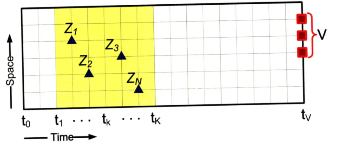
Figure 3-1: Sensor targeting over space and time: decision of deployment of sensors over the search space-time to reduce the uncertainty about the verification region.

(N: size of search space, M: size of verification region, n: number of sensing points)

compared with a much smaller-scale sensor selection problem, which is a simplified version of the problem in [10]. This comparison clearly identifies the types of systems for which the backward quantification offers a significant computational improvement over the forward one.

3.1

Sensor Selection Problems

Figure 3-1 illustrates the sensor targeting problem in a spatial-temporal grid space. The objective of sensor targeting is to deploy n sensors in the search space/time (yel-low region) in order to reduce the uncertainty in the verification region (red squares) at the verification time ty. Without loss of generality, it is assumed that each grid point is associated with a single state variable that can be directly measured. Denote the

state variable at location s as Xs, and the measurement of X, as Z,, both of which are random variables. Also, define Xs - {X1,X 2,... ,XN} and Zs - {ZI, Z2,..., ZN} the sets of all corresponding random variables over the entire search space of size

N. Likewise, V = {V, V2, ... , VM} denotes the set of random variables represent-ing the states in the verification region at tv, with M being the size of verification region. With a slight abuse of notation, this thesis does not distinguish a set of

random variables from the random vector constituted by the corresponding random variables. Measurement at location s is subject to an additive Gaussian noise that is uncorrelated with noise at any other location as well as with any of the state variables:

Z, = X,+ W, s E S [1, N] n Z (3.1)

where W, - N'(O, R,), and

P(W, W) = 0, V p C S\ {s}(3.2)

P(W,, Y) = 0, VY E XsUV.

As mentioned in section 2.1, P(A, B) AE [(A - E[A])(B - E[B])'], and P(A) P(A, A). This work assumes that the distribution of Xs U V is jointly Gaussian,

or, in a more relaxed sense, that the entropy of any set Y C (Xs U V) can be well approximated as:

=(Y) log det(P(Y))+ I log(27re). (3.3)

Also, the covariance matrix P(Xs U V) is assumed to be known in advance of making sensor targeting decisions.

The uncertainty metric in this study is entropy; uncertainty reduction over the verification region is the difference between the unconditioned entropy and the con-ditioned (on the measurement selection) entropy of V. Thus, the selection problem of choosing n grid points from the search space that will give the greatest reduction in the entropy of V can be posed as:

Forward Selection (FS)

s) = arg max I(V; Zs) R -(V) - R(V Zs)

= arg max log det P(V) -1 log det P(V Zs) (3.4)

= arg min1 log det P(VIZs)

sESn

mutual information between V and Zs. Since the prior entropy H7-(V) is identical

over all possible choices of s, the original arg max expression is equivalent to the argmin representation in the last line. Every quantity appearing in (3.4) can be computed from the given covariance information and measurement model. However, the worst-case solution technique to find s) requires an exhaustive search over the entire candidate space S,; therefore, the selection process is subject to combinatorial explosion. Note that N is usually very large for the observation targeting problem for improving weather prediction. Moreover, computing the conditional covariance P(VIZs) and its determinant requires a nontrivial computation time. In other words, a combinatorial number of computations, each of which takes a significant amount of time, are required to find the optimal solution using the FS formulation.

Given these computational issues, this thesis suggests an alternative formulation of the selection problem:

Backward Selection (BS)

s) = arg max _SES, I(Z; V) - 7-(Z ) - H-(Ze V)

=

argmax log det P(Z) - 1log det P(Zr V) (3.5)

sESn

= arg max log det (P(Xs)+ Rs) - log det (P(Xs IV) + Rs)

Instead of looking at the entropy reduction of V by Zs, this backward selection looks at the entropy reduction of Z. by V; it provides the same solution as FS, since the mutual information is commutative [35]:

Proposition 1. The forward selection and the backward selection create the same

solution:

S* = S, (3.6)

since I(V; Zs) = I(Zs; V), Vs E S,. D]

Note that P(Z

I.)

utilized a similar backward concept took advantage of this convenience. However, in the moving target tracking problems addressed in [10, 14], the verification variables are the whole state variables; in other words, V = Xs. This leads to P(XslV) = 0 with no need of computing the conditional covariances. In contrast, this work mainly considers the case in which Xs and V are disjoint, which requires conditioning processes to compute P(XsV).

Regarding computational scalability, since the worst-case solution technique to find s* is still the exhaustive search, BS is also subject to combinatorial explosion. However, the conditional covariance in the BS form can be computed by a single process that scales well with respect to n; BS can be computationally more efficient than FS. More detail on these points are given in section 3.2.

3.1.1

Ensemble-Based Adaptive Observation Targeting

The observation targeting problem for weather prediction concerns improving the weather forecast for the future time tv broadcast at the nearer future time tK (< tv), which is called "targeting time" [4], by deploying observation networks from tl through tK. While the routine sensor network, whose locations are fixed and known, is assumed to take measurements periodically (every 6 hours in practice), the targeting problem concerns deployment of a supplementary mobile network (see Figure 3-2). What is known a priori at the decision time to is the state estimate and covariance information based on past measurement histories. Since the actual values of the future measurements that affect the actual forecast error at the verification site are not available at to, the targeting considers the forecast uncertainty reduction (not the forecast error reduction) that can be quantified by estimation error covariance information without relying on the actual values of observations. Thus, the outcome of the targeting is the sensing locations/times that reduce the forecast error the most in the average sense. To address the adaptive observation targeting as a sensor selection problem presented in the previous section, it is necessary to construct the covariance field over the future time based on the a priori knowledge at time to. This section presents that procedure in the ensemble-based weather forecasting framework

4-

.

iv

I---0-to tl1-. tk "-' tK tv

-

Time---* Routine obs. already assimilated into the analysis ensemble

Future routine obs. asscociated with the Targeting

O

,& Future additional observations determined by selection process

Figure 3-2: Observation structure over the search space and time. The adaptive observation targeting problem decides the best additional sensor network over the time window [t1, tK] given the routine network that makes observations over the

same time window. The presence of routine observations between (tK, tv] is not of a practical concern, because the ultimate interest is in the quality of forecast broadcast at tK based on the actual measurement taken up to time tK. [32]

described in section 2.2.

Ensemble Augmentation and Sensor Targeting Formulation

The prior knowledge in the observation targeting problem is the analysis ensemble at

to. Since the design of the supplementary observation network is conditioned on the

presence of the routine network, the covariance field needed for the sensor selection problem is the conditional covariance field conditioned on the impact of future routine observations. Processing the observations distributed over time amounts to an EnSRF

ensemble update for the augmented forecast ensemble defined as

where

X{k = Xo + jX(t)dt, (3.8)

with Xo E RLx LE being the analysis ensemble at to. For computational efficiency,

the impact of the future routine observations is processed in advance, and the outcome of this process provides the prior information for the selection process. The routine observation matrix for the augmented system is expressed as

H~, = [ H ® IK OKnxLx], Hr E nrlxLx (3.9)

where nr is the number of routine measurements at each time step and 0 denotes the Kronecker product. Since only the covariance information is needed (and available) for targeting, incorporation of the future routine networks involves only the perturbation ensemble update

Xag

f

Xug -(I- KaugHaug)Xaug (3.10)

without updating the ensemble mean. In the sequential EnSRF scheme, this process can be performed one observation at a time.

Xa,, will be utilized to construct the prior covariance matrix for the sensor se-lection problem. Since the selection problem only concerns the search space and the verification region, it deals with a submatrix of the Xa

aug

Xxsuv = (7,..., ~x , (,.t,• , (3.11)

where (.) E RALE represents the row vector of Xaug corresponding to the subscribed

variable. Using this ensemble, the covariance matrix of Y E {Y,..., Yk} C Xs U V can be evaluated as

P,(Y) = [, -. ,: k T,,"~ ( /(LE - 1). (3.12)

The distribution of Xs U V is not jointly Gaussian in general due to nonlinearity of the dynamics; however, the entropy information is assumed to be well represented by the