HAL Id: halshs-00118801
https://halshs.archives-ouvertes.fr/halshs-00118801
Submitted on 6 Dec 2006
HAL is a multi-disciplinary open access archive for the deposit and dissemination of sci-entific research documents, whether they are pub-lished or not. The documents may come from teaching and research institutions in France or abroad, or from public or private research centers.
L’archive ouverte pluridisciplinaire HAL, est destinée au dépôt et à la diffusion de documents scientifiques de niveau recherche, publiés ou non, émanant des établissements d’enseignement et de recherche français ou étrangers, des laboratoires publics ou privés.
Understanding the processes of firm growth - a closer
look at serial growth rate correlation
Alex Coad
To cite this version:
Alex Coad. Understanding the processes of firm growth - a closer look at serial growth rate correlation. 2006. �halshs-00118801�
Maison des Sciences Économiques, 106-112 boulevard de L'Hôpital, 75647 Paris Cedex 13
http://mse.univ-paris1.fr/Publicat.htm
Centre d’Economie de la Sorbonne
UMR 8174
Understanding the Processes of Firm Growth -A Closer Look at Serial Growth Rate Correlation
Alex COAD
Understanding the Processes of Firm Growth - a Closer
Look at Serial Growth Rate Correlation
∗
Alex Coad
?? MATISSE, Univ. Paris 1 Panth´eon-Sorbonne, Paris, France
LEM, Sant’Anna School of Advanced Studies, Pisa, Italy
Cahiers de la MSE
S´
erie rouge
Cahier num´
ero R06051
Abstract
Serial correlation in annual growth rates carries a lot of information on growth pro-cesses - it allows us to directly observe firm performance as well as to test hypotheses. Using a 7-year balanced panel of 10 000 French manufacturing firms, we observe that small firms typically are subject to negative correlation of growth rates, whereas larger firms display positive correlation. Furthermore, we find that those small firms that ex-perience extreme positive or negative growth in any one year are unlikely to repeat this performance in the following year.
COMPRENDRE LE PROCESSUS DE CROISSANCE DES FIRMES : UNE AUTRE REGARD SUR L’AUTOCORRELATION
R´esum´e: L’autocorr´elation dans les taux de croissance annuels fournit beaucoup d’informations sur les processus de croissance – elle nous permet d’observer directement la performance des firmes ainsi que de tester des hypoth`eses. Analysant un panel de 10 000 entreprises manufacturi`eres fran¸caises sur 7 ans, nous observons que la croissance des petites entreprises est typiquement marqu´ee par une autocorr´elation n´egative, tandis que les firmes plus grandes montrent une au-tocorr´elation positive. De plus, nous observons que ces petites entreprises qui ont une croissance extrˆeme (positive ou n´egative) ne peuvent vraisemblablement pas reproduire cette performance l’ann´ee suivante.
JEL codes: L11, L25
Keywords: Serial correlation, firm growth, quantile regression
Mots cl´es: Autocorr´elation, croissance des firmes, r´egression par quantile
1
Introduction
“[S]erial correlation in firm growth rates ... is of considerable economic interest and deserves to be examined in its own right.” Singh and Whittington (1975, p. 17)
∗Thanks go to Bernard Paulr´e for helpful comments. The usual caveat applies.
Corresponding Author : Alex Coad, MATISSE, Maison des Sciences Economiques, 106-112 Bd. de l’Hˆopital,
A lot of information on the processes of firm growth can be obtained by studying serial correlation in growth rates. At first glance, it allows us to directly observe the evolution of industries by better understanding patterns of year-on-year growth at the firm-level. Such research may have policy implications if, for example, it is desirable to prevent large firms from experiencing cumulative growth, or if one should want to investigate the ability of small firms to generate durable employment, i.e. jobs that have not disappeared by the following year.
Another more subtle motivation for studying serial correlation is that it allows us to judge between theories by comparing the hypothetical predictions with the empirically-observed regularities. First of all, if it were observed to be significant, the existence of serial correlation would lead us to reject Gibrats law of proportionate effect and the associated stochastic models of industry evolution. This strand of the literature treats firm growth as a purely stochastic phenomenon in which a firm’s size at any time is simply the product of previous growth shocks. Following Sutton (1997), we define the size of a firm at time t by xt, and represent growth by
the random variable εt (i.e. the ‘proportionate effect’) to obtain:
xt− xt−1 = εt· xt−1
whence:
xt = (1 + ε)xt−1 = x0(1 + ε1)(1 + ε2) . . . (1 + εt) (1)
According to equation (1), a firm’s size can be seen as the simple multiplication of independent growth shocks. This simple model has become a popular benchmark for modelling industrial evolution because, among other properties, it is able to generate the observed log-normal firm-size distribution, and also the proposition that expected growth is independent of firm-size does find empirical support (roughly speaking). However, such a model would be inappropriate if the assumption of serial independence of growth rates does not find reasonable empirical support.
Second, the notion of a firm- or industry-specific optimal size and the related adjustment cost hypothesis of firm growth can be rejected by looking at the characteristics of serial growth correlation. The traditional, static representation of the firm considered it as having an optimal size determined in a trade-off between production technology and decreasing returns to bureaucratization. This conceptualization of firms having an optimal size was then extended to the case of growing firms. According to this approach, firms have a target size that they tend towards, but the existence of non-linear adjustment costs prohibits them from instantly attaining their ideal size. Instead, they grow gradually by equating at the margin the gains from having a larger size and the costs of growing. If this theory is to be believed, we should expect to find a positive autocorrelation in growth rates as firms approach their optimal size. However, in reality we do not always observe positive autocorrelation in annual growth rates which leads us to doubt the validity of this theory.
Third, looking at autocorrelation statistics will allow us to judge between the different models that attempt to explain the heavy-tailed distribution of annual firm growth rates. The explanation offered by Bottazzi and Secchi (2006) hinges on the notion of increasing returns in the growth process, which would lead us to expect positive autocorrelation in annual growth rates. The explanation offered by Coad (2006), however, considers that firms grow by the addition of lumpy resources. It follows from the discrete and interdependent nature of these resources that the required additions in any one year are occasionally rather large. In this case, we would expect a small negative autocorrelation of annual growth rates.
Another motivation for this study is to observe what happens to those firms that grow extremely fast. Indeed, a robust ‘stylised fact’ that has emerged only recently is that annual firm growth rates distributions are remarkably fat-tailed and can be approximated by the Laplace distribution (Stanley et al. 1996, Bottazzi and Secchi 2003, Bottazzi et al. 2005, Bottazzi et al. 2006). A considerable proportion of employment creation takes place within just a handful of fast-growing firms. Conventional regression techniques that focus on what happens to the ‘average firm’, and that dismiss extreme events as ‘outliers’, may thus be inappropriate. In this study we therefore include semi-parametric regression techniques (i.e. quantile regression) to tackle this issue.
This paper provides several novel results. In particular, we observe that autocorrelation dynamics vary with firm size, such that whilst large firms experience positive feedback in year-to-year growth rates, the growth of smaller firms is marked by an erratic, ‘start-and-stop’ dynamics. Indeed, small and large firms appear to operate on different ‘frequencies’. For those small firms that experience extreme growth in one year, significant negative correlation indi-cates that they are quite unlikely to repeat this performance in the following year. Larger firms undergoing extreme growth events, however, do not experience such strong autocorrelation.
Section 2 reviews the previous literature relating to this subject, and section 3 presents the database. In section 4, we begin with some summary statistics and results using conven-tional regressions, and then apply quantile regression techniques. Section 5 concludes with a discussion of our findings.
2
Literature review
The relevant empirical questions in this section are the sign, the magnitude, and also the time-scale of serial correlation in the growth rates of firms.
Early empirical studies into the growth of firms measured serial correlation when growth was measured over a period of 4 to 6 years. Positive autocorrelation of 33% was observed by Ijiri and Simon (1967) for large US firms, and a similar magnitude of 30% was reported by Singh and Whittington (1975) for UK firms. However, much weaker autocorrelation was later reported in comparable studies by Kumar (1985) and Dunne and Hughes (1994).
More recently, availability of better datasets has encouraged the consideration of annual autocorrelation patterns. Indeed, persistence should be more visible when measured over shorter time horizons. However, the results are quite mixed. Positive serial correlation has often been observed, in studies such as those of Chesher (1979) and Geroski et al. (1997) for UK quoted firms, Wagner (1992) for German manufacturing firms, Weiss (1998) for Austrian farms, Bottazzi et al. (2001) for the worldwide pharmaceutical industry, and Bottazzi and Secchi (2003) for US manufacturing. On the other hand, negative serial correlation has also been reported some examples are Boeri and Cramer (1992) for German firms, Goddard et
al. (2002) for quoted Japanese firms, Bottazzi et al. (2003) for Italian manufacturing, and
Bottazzi et al. (2005) for French manufacturing. Still other studies have failed to find any significant autocorrelation in growth rates (see Almus and Nerlinger (2000) for German start-ups, Bottazzi et al. (2002) for selected Italian manufacturing sectors, Geroski and Mazzucato (2002) for the US automobile industry, and Lotti et al. (2003) for Italian manufacturing firms). To put it mildly, there does not appear to be an emerging consensus.
Another subject of interest (also yielding conflicting results) is the number of relevant lags to consider. Chesher (1979) and Bottazzi and Secchi (2003) found that only one lag was significant, whilst Geroski et al. (1997) find significant autocorrelation at the 3rd lag (though
not for the second). Bottazzi et al. (2001) find positive autocorrelation for every year up to and including the seventh lag, although only the first lag is statistically significant.
It is perhaps remarkable that the results of the studies reviewed above have so little in common. It is also remarkable that previous research has been so little concerned with this question. Indeed, instead of addressing serial correlation in any detail, often it is controlled away as a dirty residual, a blemish on the natural growth rate structure. The baby is thus thrown out with the bathwater. In our view, the lack of agreement would suggest that, if there are any regularities in the serial correlation of firm growth, they are more complex than the standard specification would be able to detect (i.e. that there is no ‘one’ serial correlation coefficient that applies for all firms). We therefore consider how serial correlation changes with two aspects of firms – their size, and their growth rate – and our results, though preliminary, are nonetheless encouraging.
3
Database
This research draws upon the EAE databank collected by SESSI and provided by the French Statistical Office (INSEE).1 This database contains longitudinal data on a virtually exhaustive
panel of French firms with 20 employees or more over the period 1989-2002. We restrict our analysis to the manufacturing sectors. For statistical consistency, we only utilize the period 1996-2002 and we consider only continuing firms over this period. Firms that entered midway through 1996 or exited midway through 2002 have been removed. Since we want to focus on internal, ‘organic’ growth rates, we exclude firms that have undergone any kind of modification of structure, such as merger or acquisition. Because of limited information on restructuring activities and in contrast to some previous studies (e.g. Bottazzi et al. 2001), we do not attempt to construct ‘super-firms’ by treating firms that merge at some stage during the period under study as if they had been merged from the start of the period. Firms are classified according to their sector of principal activity.2 To start with we had observations for around 22000 firms
per year for each year of the period.3 In the final balanced panel constructed for the period
1996-2002, we have exactly 10000 firms for each year.
4
Analysis
4.1
Summary statistics
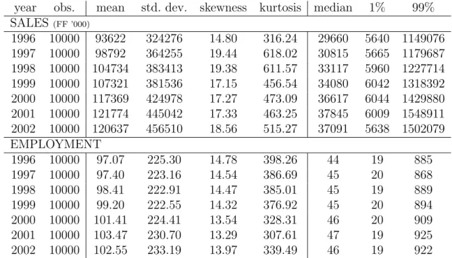
We begin by looking at some summary statistics of firms in our database (see table 1). First, in keeping with the elementary ‘stylized facts’ of industry stucture, we observe that the firm-size distribution is right-skewed (compare the mean and the median, look also at the skewness and kurtosis statistics). Second, the distribution appears to be roughly stationary, although in the Sales statistics there is an steady upward drift due to economic development and inflation.
Our two measures of size and growth are sales and number of employees, which are highly correlated with each other.4 Figures 1 and 2 present the distributions of sales and employment
1The EAE databank has been made available to the author under the mandatory condition of censorship
of any individual information.
2The French NAF classification matches with the international NACE and ISIC classifications. 322319, 22231, 22305, 22085, 21966, 22053, and 21855 firms respectively
4The correlation between sales and number of employees is 0.8404 (with N =70 000), and the correlation
Table 1: Summary statistics of the firm size distribution
year obs. mean std. dev. skewness kurtosis median 1% 99% SALES (FF ’000) 1996 10000 93622 324276 14.80 316.24 29660 5640 1149076 1997 10000 98792 364255 19.44 618.02 30815 5665 1179687 1998 10000 104734 383413 19.38 611.57 33117 5960 1227714 1999 10000 107321 381536 17.15 456.54 34080 6042 1318392 2000 10000 117369 424978 17.27 473.09 36617 6044 1429880 2001 10000 121774 445042 17.33 463.25 37845 6009 1548911 2002 10000 120637 456510 18.56 515.27 37091 5638 1502079 EMPLOYMENT 1996 10000 97.07 225.30 14.78 398.26 44 19 885 1997 10000 97.40 223.16 14.54 386.69 45 20 868 1998 10000 98.41 222.91 14.47 385.01 45 19 889 1999 10000 99.20 222.55 14.32 376.92 45 20 894 2000 10000 101.41 224.41 13.54 328.31 46 20 909 2001 10000 103.47 230.70 13.29 307.61 47 19 925 2002 10000 102.55 233.19 13.97 339.49 46 19 922 0.001 0.01 0.1 1 -3 -2 -1 0 1 2 prob.
conditional growth rate 1998 2000 2002
Figure 1: Distribution of sales growth rates (source: Bottazzi et al., 2005)
0.001 0.01 0.1 1 -2 -1.5 -1 -0.5 0 0.5 1 1.5 2 prob.
conditional growth rate 1998 2000 2002
Figure 2: Distribution of employment growth rates (source: author’s elaboration)
growth rates, where these growth rates are cleaned of size dependence, serial correlation and heteroskedasticity effects according to the procedure described in Bottazzi et al. (2005). The main point of interest here is that the distribution is fat-tailed and appears to be approximately ‘tent-shaped’ on logarithmic axes. This testifies that relatively large growth events in any year occur not altogether infrequently.
4.2
Regression analysis
In keeping with previous studies, we define our dependent variable GROW T H as the log-difference of size:
GROW T Hi(t) = log(SIZEi(t)) − log(SIZEi(t − 1)) (2)
Table 2: OLS estimation of equation (3), taking 3 lags t β1 β2 β3 SALES 2000 -0.2092 -0.0940 -0.0180 (SE) (0.0239) (0.0194) (0.0171) 2001 -0.2161 -0.0542 0.0049 (SE) (0.0235) (0.0191) (0.0148) 2002 -0.2514 -0.1283 -0.0353 (SE) (0.0292) (0.0235) (0.0166) EMPL 2000 -0.1133 0.0367 0.0478 (SE) (0.0289) (0.0164) (0.0173) 2001 -0.1177 0.0186 0.0449 (SE) (0.0376) (0.0139) (0.0148) 2002 -0.1093 -0.0128 0.0406 (SE) (0.0251) (0.0286) (0.0179)
Table 3: MAD estimation of equation (3), tak-ing 3 lags t β1 β2 β3 SALES 2000 -0.0417 0.0093 0.0276 (SE) (0.0061) (0.0063) (0.0057) 2001 -0.0551 0.0183 0.0366 (SE) (0.0059) (0.0060) (0.0058) 2002 -0.0552 -0.0272 0.0089 (SE) (0.0063) (0.0063) (0.0062) EMPL 2000 0.0133 0.0548 0.0460 (SE) (0.0059) (0.0064) (0.0064) 2001 0.0113 0.0213 0.0278 (SE) (0.0055) (0.0055) (0.0058) 2002 0.0000 0.0000 0.0000 (SE) (0.0056) (0.0054) (0.0053)
for firm i at time t, where SIZE is measured either in terms of sales or employees. We then estimate the following regression equation:
GROW T Hi(t) = α0+ α1MEAN SIZEi+ K
X
k=1
βkGROW T Hi(t − k) + y(t) + ²i(t). (3)
Given that the Gibrat Law literature has identified a dependence of growth rates upon firm size, we introduce MEAN SIZE as a control variable. To avoid the possibility of spurious results due to the ‘regression fallacy’ (see e.g. Friedman, 1992), MEAN SIZE here is measured as the log of the mean number of employees for the whole period 1996-2002. In the rest of this paper, we report values for the βkonly, and will repeatedly use the variable MEAN SIZE as
defined here.
To begin with, we estimate equation (3) by OLS, but since the residuals are known to be approximately Laplace distributed OLS is likely to perform relatively poorly (Bottazzi et
al. 2005). We therefore prefer the results obtained by Minimum Absolute Deviation (MAD)
estimation of equation (3). Regression results are reported in tables 2 and 3. When growth is measured in terms of sales, we observe a small negative autocorrelation for the first lag, in the order of -5%. The second lag is smaller, sometimes significant, but variable across the three years; and the third lag is small and positive. Regarding employment growth, we observe a small yet positive and statistically significant correlation coefficient for the average firm, for each of the first three lags.
However, it has previously been noted that one calendar year is an arbitrary period over which to measure growth (see the discussion in Geroski, 2000). We will now look at growth rate autocorrelation over periods of two and three years, by MAD estimation of equation (3). The results are presented in tables 4 and 5. When we measure growth over periods of two or three years, we obtain quite different results. Regarding autocorrelation of sales growth, we obtain a positive and significant coefficient when growth is measured over a three-year interval, which
Table 4: MAD estimation of equation (3), with sales growth measured over different periods
t β1 β2 00-02 98-00 96-98 -0.0444 0.0276 (0.0066) (0.0067) 99-01 97-99 0.0028 (0.0063) 98-00 96-98 -0.0075 (0.0066) 99-02 96-99 0.0161 (0.0067)
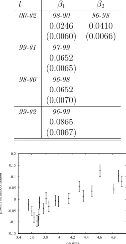
Table 5: MAD estimation of equation (3), with employment growth measured over different pe-riods t β1 β2 00-02 98-00 96-98 0.0246 0.0410 (0.0060) (0.0066) 99-01 97-99 0.0652 (0.0065) 98-00 96-98 0.0652 (0.0070) 99-02 96-99 0.0865 (0.0067) -0.2 -0.15 -0.1 -0.05 0 0.05 0.1 3.4 3.6 3.8 4 4.2 4.4 4.6 4.8 5
growth rate autocorrelation
log(size)
Figure 3: Autocorrelation of annual sales growth
-0.15 -0.1 -0.05 0 0.05 0.1 0.15 0.2 3.4 3.6 3.8 4 4.2 4.4 4.6 4.8 5
growth rate autocorrelation
log(size)
Figure 4: Autocorrelation of annual employment growth
contrasts with the results presented in table 3 for annual data. In addition, the coefficients for employment growth autocorrelation are much larger when growth is measured over two or three years.
These results highlight some important features that should be kept in mind when in-vestigating serial correlation. First, both the magnitude and even the sign of the observed autocorrelation coefficients are sensitive to the accounting period used. We should be reluc-tant to speak of ‘mean reversion’ in the growth process generally, for example, if we observe negative autocorrelation in annual growth rates, because these findings may not be robust to changes in time periods. Second, the conventional accounting period of one year is arbi-trary and does not correspond to any meaningful duration of economic activity. Given these important qualifications, our following analysis is nonetheless able to provide useful insights into the growth process because it explores systematic variation in serial correlation patterns, conditional on firm size and conditional on growth rates.
4.3
Does autocorrelation vary with firm size?
As firms grow, they undergo many fundamental changes (Greiner, 1998). Whilst smaller firms are characteristically flexible, larger firms are more routinized, more inert and less able to adapt. In large firms, everything takes place on a larger scale, there is less reason to fear a ‘sudden death’, and the time-scale of strategic horizons extend much further than for a smaller counterpart. Larger firms may well have longer-term investment projects that unfold over a period of several years, whereas smaller firms can adjust much more rapidly. It is therefore meaningful to suppose that differences in the behavior of large firms and smaller firms will also be manifest in their respective growth processes. It has previously been conjectured that large and small firms operate on a different ‘frequency’ or time-scale, and respond to different stimuli (Hannan and Freeman, 1984).5 However, to my knowledge, no empirical study has
explicitly considered this relationship. The results in Dunne and Hughes (1994: table VI) and in Wagner (1992: table II) would appear to lean in this direction, but the authors fail to comment upon this possibility. The aim of this section is thus to compare growth rate autocorrelation among firms of different sizes.
We sort firms into 20 equipopulated bins according to their MEAN SIZE as defined before, and calculate their growth rate autocorrelation by MAD estimation of equation (3). The evidence presented in figures 3 and 4 would seem to support the hypothesis that annual growth rate autocorrelation varies with size, being negative, on average, for small firms and positive for larger ones. Further evidence in support of this hypothesis will also be presented in what follows.
We should be careful how we interpret these results. It may not be meaningful to say that large firms have positive feedback and smaller firms have negative feedback in their growth dynamics because, as discussed previously, it is possible that the magnitudes and signs of the autocorrelation coefficients would change if we were to measure growth over a different time period. However, one thing that we can infer from these results is that large firms and small firms operate on different time scales.
4.4
Quantile regression analysis
As an extension to the observation that the distribution of growth rates is heavy-tailed, in this section we ask the question: “how does serial correlation affect the growth processes of these extreme-growth firms?” Conventional regression techniques such as OLS focus on the ‘average firm’, assume normally-distributed residuals and are not robust to outliers. In fact, extreme observations are frequently dropped from the analysis. In our case, however, the distribution of firm growth rates is fat-tailed, resembling the Laplace density rather than the Gaussian. Furthermore, we explicitly want to focus on those few firms that experience extreme growth events because they make a disproportionate contribution to employment growth and market share turnover. As opposed to standard regression techniques, quantile regression analysis appears appropriate here because it provides a parsimonious description of the entire conditional growth rate distribution (see Koenker and Hallock (2001) for an
5To be precise, Hannan and Freeman write about: “the proposition that time-scales of selection processes
stretch with size. . . One way to visualize such a relationship is to consider environmental variations as composed of a spectrum of frequencies of varying lengths - hourly, daily, weekly, annually, etc. Small organizations are more sensitive to high-frequency variations than large organizations. For example, short-term variations in the availability of credit may be catastrophic to small businesses but only a minor nuisance to giant firms. To the extent that large organizations can buffer themselves against the effects of high-frequency variations, their viability depends mainly on lower-frequency variations.” Hannan and Freeman, 1984:161
-0.3 -0.25 -0.2 -0.15 -0.1 -0.05 0 0.05 0.1 0 0.2 0.4 0.6 0.8 1 autocorrelation coefficient quantile sales empl
Figure 5: regression quantiles for sales and employment autocorrelation coefficients
Table 6: Quantile regression estimation of equation (3) for the 10%, 25%, 50%, 75% and 90% quantiles, allowing for only one lag in serial correlation.
10% 25% 50% 75% 90% Sales gr. β1 -0.1343 -0.0713 -0.0458 -0.0639 -0.1372 (t-stat) -12.34 -16.67 -15.51 -15.76 -11.99 Pseudo-R2 0.0304 0.0261 0.0189 0.0229 0.0267 Empl. gr. β1 -0.0895 -0.020315 1.58e-6 -0.0077 -0.0771 (t-stat) -8.71 -5.35 1.05 -1.56 -5.46 Pseudo-R2 0.0094 0.0044 0.0007 0.0090 0.0145
introduction to quantile regressions, see also Coad and Rao (2006) for an application). It will thus be possible to examine serial correlation patterns for firms of all quantiles, including autocorrelation dynamics of extreme growth firms.
The quantile regression results are presented in table 6, and a summary representation is provided in figure 5. The coefficients can be interpreted as the partial derivative of the conditional quantile of y with respect to particular regressors, δQθ(yit|xit)/δx. Evaluated at the
median, we observe that there is only slight negative autocorrelation in sales growth and totally insignificant autocorrelation in employment growth. The story does not end there, however, because the serial correlation coefficient estimates vary considerably across the conditional growth rate distribution. For firms experiencing dramatic losses in sales or employment at time t, the sharply negative coefficient implies that in the previous period t − 1 these firms were probably experiencing above-average growth. Similarly, for those fastest-growing firms at time t, the negative coefficient estimate indicates that these firms probably performed relatively poorly in the previous period t − 1. It would appear then that, although in any one year there are some firms that undergo significant growth events, these firms are unlikely to repeat this performance.6 According to this evidence, it would appear that the better analogy
would probably be that of the ‘hare and tortoise’ rather than notions of cumulative ‘snowball effect’ dynamics or even serial independence of growth rates.
4.5
Robustness across size groups
Are the previous results robust across size? Or is the relationship displayed in figure 5 just the result of aggregating firms of different sizes – where smaller firms are the extreme growers and it is these same firms that experience the negative autocorrelation? It does not appear, for this dataset, that growth rate variance decreases dramatically with size (compare Bottazzi
et al. (2005) with Bottazzi and Secchi (2003)). Nevertheless, in this section we will investigate
possible heterogeneity across size classes by applying quantile regression analysis to different size groups. We sort and split the firms into 10 size groups according to their MEAN SIZE. as defined previously. We then explore the regression quantiles for each of these 10 groups. Results are presented in table 7 and figures 6 (sales growth) and 7 (employment growth).
The results are reasonably consistent whether we consider sales growth or employment growth. For the larger firms, the results support the previous finding that, on average, these firms experience a slightly positive autocorrelation in annual growth rates. Even as we move to the extremes of the conditional distribution, the autocorrelation coefficient does not change too dramatically. Smaller firms, however, typically experience negative correlation which is moderate near the median but quite pronounced towards the extreme quantiles.
4.6
Robustness to sectoral disaggregation
Rigourous empirical methodology requires us to also ensure that these results are not due to aggregation over heterogeneous industries. In this section, we report quantile regression
6One potential problem that we thought deserved investigation was the possibility of data entry errors.
Despite the INSEEs reputation for providing high-quality data, we were concerned that there could be cases of omitted numbers in which a firm’s sales (or employees) were observed to shrink by tenfold in one year and grow by tenfold in the next. Where we found such cases, we checked for consistency with other corresponding variables (e.g. value added, employees etc). As it happens, the database appeared consistent under scrutiny and we are pleased to acknowledge that our suspicions were a waste of time.
Table 7: Quantile regression estimation of equation (3) for the 10%, 25%, 50%, 75% and 90% quantiles for 10 size groups (1 = smallest), allowing for only one lag in serial correlation.
10% 25% 50% 75% 90% Sales gr. 1: β1 -0.1984 -0.1380 -0.1084 -0.0980 -0.1775 (t-stat) -5.65 -8.57 -10.94 -7.08 -6.36 2: β1 -0.2706 -0.1566 -0.0974 -0.1324 -0.2147 (t-stat) -6.63 -12.98 -10.28 -9.54 -5.22 3: β1 -0.2229 -0.1426 -0.1022 -0.1236 -0.2071 (t-stat) -5.36 -12.11 -13.68 -8.61 -4.99 4: β1 -0.1742 -0.1144 -0.0708 -0.1049 -0.1928 (t-stat) -6.25 -10.33 -8.63 -6.62 -4.71 5: β1 -0.0650 -0.0239 -0.0482 -0.0785 -0.1626 (t-stat) -2.01 -2.04 -4.69 -5.88 -4.23 6: β1 -0.0966 -0.0497 -0.0261 -0.0345 -0.1153 (t-stat) -3.36 -3.59 -2.45 -2.44 -3.38 7: β1 -0.1440 -0.0701 -0.0447 -0.0469 -0.1197 (t-stat) -4.24 -4.98 -5.70 -3.47 -3.28 8: β1 -0.0285 0.0057 0.0083 -0.0132 -0.0503 (t-stat) -0.88 0.39 0.83 -0.90 -1.13 9: β1 -0.1103 -0.0291 0.0255 0.0194 -0.0400 (t-stat) -2.92 -2.01 2.53 1.43 -1.04 10: β1 0.0255 0.0920 0.0862 0.0709 0.0779 (t-stat) 0.64 6.93 7.96 3.81 2.11 Empl. gr. 1: β1 -0.1414 -0.0436 0.0000 -0.0645 -0.1182 (t-stat) -3.36 -10.28 0.00 -10.03 -3.47 2: β1 -0.2482 -0.1412 0.0000 -0.0973 -0.2019 (t-stat) -6.96 -10.68 0.00 -7.72 -5.14 3: β1 -0.2384 -0.1528 -0.0820 -0.1584 -0.3008 (t-stat) -5.60 -9.69 -13.70 -9.85 -6.23 4: β1 -0.1135 -0.0673 0.0000 -0.0855 -0.1966 (t-stat) -4.19 -5.28 0.00 -4.43 -3.97 5: β1 -0.0536 -0.0172 0.0000 -0.0603 -0.1660 (t-stat) -1.54 -1.90 0.00 -6.92 -3.98 6: β1 -0.0663 -0.0051 0.0000 0.0032 -0.1066 (t-stat) -2.52 -1.04 0.00 0.26 -2.81 7: β1 -0.0924 0.0157 0.0137 0.0514 0.0154 (t-stat) -2.69 2.59 5.97 3.75 0.40 8: β1 0.0410 0.0645 0.0755 0.1165 0.0944 (t-stat) 1.60 4.86 9.79 8.41 2.63 9: β1 0.0450 0.0449 0.0932 0.1700 0.1811 (t-stat) 1.37 3.48 13.01 11.6 4.95 10: β1 0.0888 0.1194 0.1770 0.1996 0.1943 (t-stat) 1.82 9.60 32.09 18.93 6.92
-0.3 -0.25 -0.2 -0.15 -0.1 -0.05 0 0.05 0.1 0 0.2 0.4 0.6 0.8 1 autocorrelation coefficient quantile 1 2 3 4 5 6 7 8 9 10
Figure 6: regression quantiles for sales growth autocorrelation coefficients across the 10 size groups (group ‘1’ = smallest group)
-0.3 -0.2 -0.1 0 0.1 0.2 0 0.2 0.4 0.6 0.8 1 autocorrelation coefficient quantile 1 2 3 4 5 6 7 8 9 10
Figure 7: regression quantiles for employment growth autocorrelation coefficients across the 10 size groups (group ‘1’ = smallest group)
T able 8: Description of the 2-digit man ufacturing sectors studied (source: Bottazzi et al . 2005) ISIC class Description No. obs. Mean size (1996) ( ¿ ’000 in 2002) 17 Man uf. of textiles 730 9703 18 Man uf. of w earing apparel, dressing and dy eing of fur 498 9623 19 T anning and dressing of leather, man uf. of luggage, handbags, .. . 205 14629 20 Man uf. of w o o d and pro ducts of w o o d and cork, except furniture; .. . 314 9083 21 Man uf. of pap er and pap er pro ducts 364 22428 22 Publishing, prin ting and repro duction of recorded media 820 13745 23 Man uf. of cok e, refined p etroleum pro ducts and n uclear fuel 19 73547 24 Man uf. of chemicals and chemical pro ducts 496 52378 25 Man uf. of rubb er and plastics pro ducts 685 17964 26 Man uf. of other non-metallic mineral pro ducts 426 21624 27 Man uf. of basic metals 265 34411 28 Man uf. of fabricated metal pro ducts, except mac hinery and equipmen t 2276 8041 29 Man uf. of mac hinery and equipmen t n.e.c. 987 19343 30 Man uf. of office, accoun ting and computing mac hinery 23 39850 31 Man uf. of electrical mac hinery and apparatus n.e.c. 357 26740 32 Man uf. of radio, television and comm unication equipmen t and apparatus 218 25159 33 Man uf. of medical, precision and optical instrumen ts, w atc hes and clo cks 354 12452 34 Man uf. of motor vehicles, trailers and semi-trailers 280 49195 35 Man uf. of other transp ort equipmen t 137 68192 36 Man uf. of furniture; man ufacturing n.e.c. 546 14411
Table 9: Quantile regression estimation of equation (3) for the 10%, 25%, 50%, 75% and 90% quantiles for 20 2-digit sectors (17-36), allowing for only one lag in serial correlation.
10% 25% 50% 75% 90% 10% 25% 50% 75% 90% Sales gr. Empl. gr. 17: β1 0.0588 0.0221 0.0003 -0.0094 -0.0303 -0.0217 0.0128 0.0003 0.0294 -0.0191 (t-stat) 2.24 1.69 0.02 -0.57 -0.66 -0.50 0.92 1.33 1.85 -0.45 18: β1 -0.1438 -0.0392 -0.0284 -0.05 -0.1170 -0.0907 -0.0312 0.0000 -0.0699 -0.1097 (t-stat) -3.30 -2.56 -2.21 -2.38 -2.10 -2.13 -1.86 0.00 -4.52 -1.82 19: β1 -0.1227 -0.0296 -0.0032 -0.0967 -0.1718 -0.2684 -0.1256 -0.0379 -0.0727 -0.1550 (t-stat) -2.56 -1.42 -0.22 -4.95 -2.08 -3.08 -5.19 -2.98 -2.00 -1.67 20: β1 -0.0458 -0.0188 0.0144 0.0383 -0.1454 -0.1578 -0.0531 -0.0019 -0.0319 -0.0896 (t-stat) -1.09 -0.98 0.68 1.63 -1.86 -2.92 -1.80 -0.79 -0.88 -1.12 21: β1 -0.2197 -0.0961 -0.0563 -0.1180 -0.2096 -0.1027 -0.0304 -0.0001 0.0018 -0.0531 (t-stat) -5.86 -4.39 -4.01 -5.80 -3.46 -1.80 -1.74 -1.29 0.12 -0.82 22: β1 -0.1691 -0.0574 -0.0194 -0.0374 -0.0903 -0.1506 -0.0753 0.0000 -0.0507 -0.1484 (t-stat) -4.12 -4.95 -2.85 -3.57 -2.48 -2.84 -5.32 0.00 -3.20 -3.72 23: β1 0.0961 0.1317 0.1883 0.1523 0.1098 -0.0899 0.0683 0.1788 0.1926 0.0678 (t-stat) 0.20 1.80 9.09 5.16 0.12 -0.22 0.80 2.52 1.98 0.27 24: β1 -0.0667 -0.0155 -0.0100 -0.0272 -0.0558 0.0634 0.0550 0.0587 0.0818 0.0068 (t-stat) -1.46 -1.01 -0.84 -1.48 -1.14 1.34 3.40 7.66 4.79 0.10 25: β1 -0.1346 -0.0582 -0.0246 -0.0440 -0.1126 -0.1009 -0.0262 0.0000 0.0091 -0.0361 (t-stat) -2.50 -3.93 -2.34 -2.87 -3.05 -2.06 -1.50 0.00 0.46 -0.82 26: β1 -0.0685 -0.3990 -0.0239 -0.0686 -0.1429 -0.1252 -0.0216 -0.0003 -0.0689 -0.1483 (t-stat) -1.30 -2.31 -2.20 -3.31 -2.60 -1.77 -1.13 -0.56 -3.34 -2.45 27: β1 -0.1552 -0.1052 -0.0189 0.0094 0.0096 -0.0744 0.0194 0.0115 0.0455 0.0176 (t-stat) -2.42 -5.02 -0.79 0.29 0.19 -3.05 2.02 3.24 3.58 0.60 28: β1 -0.1801 -0.1219 -0.1003 -0.1153 -0.1748 -0.1262 -0.0485 -0.0005 -0.0353 -0.1284 (t-stat) -7.71 -13.85 -14.57 -12.46 -7.07 -6.97 -5.73 -6.37 -3.14 -4.27 29: β1 -0.2043 -0.1438 -0.1062 -0.1354 -0.1874 -0.0909 -0.0084 0.0006 -0.0028 -0.0758 (t-stat) -4.91 -8.98 -12.20 -9.37 -4.34 -2.91 -0.77 2.21 -0.18 -1.87 30: β1 0.0074 -0.0959 0.0194 0.0593 -0.1050 -0.3232 -0.0403 0.1071 0.1416 0.2377 (t-stat) 0.30 -0.70 0.14 0.33 -0.31 -0.86 -0.20 1.49 1.23 0.22 31: β1 -0.0551 -0.0749 -0.0437 -0.0602 -0.1216 -0.0490 0.0227 0.0172 0.0735 0.1041 (t-stat) -1.00 -2.69 -2.91 -2.39 -2.11 -0.87 1.09 1.26 3.07 0.1041 32: β1 -0.1094 -0.0904 -0.0610 -0.0228 -0.0538 -0.0106 -0.0138 0.0384 0.0692 0.1172 (t-stat) -1.31 -2.42 -1.88 -0.93 -0.91 -0.14 -0.62 1.66 1.87 1.16 33: β1 -0.1573 -0.1179 -0.0763 -0.0779 -0.1457 -0.1160 0.0053 0.0000 0.0895 0.0967 (t-stat) -2.60 -5.47 -5.33 -2.63 -1.87 -2.03 0.22 0.00 3.45 1.37 34: β1 -0.0696 -0.0472 -0.0193 -0.0386 -0.0438 -0.1472 -0.0298 0.0245 0.0592 0.0715 (t-stat) -1.09 -1.98 -0.92 -1.83 -0.51 -2.51 -1.12 1.09 1.75 0.83 35: β1 -0.2325 -0.1190 -0.1097 -0.1439 -0.2830 -0.0719 0.0036 0.0443 0.0228 -0.1280 (t-stat) -2.52 -3.53 -4.51 -3.74 -1.90 -0.59 0.15 2.09 0.61 -0.89 36: β1 0.0052 -0.0304 -0.0172 -0.0588 -0.1527 0.0113 0.0087 0.0039 -0.0482 -0.1278 (t-stat) 0.17 -2.51 -1.53 -3.25 -2.60 0.32 0.61 1.40 -1.87 -2.48
results for 20 2-digit industries. Summary information on these sectors is provided in table 8 and the results are presented in table 9.
Generally speaking, the properties that were visible at the aggregate level are also visible for 2-digit industries. Firms near the median experience only moderate autocorrelation (either positive or negative), whereas firms at the extreme quantiles of the conditional growth rate distribution experience much stronger forces of negative autocorrelation. Although sectoral disaggregation does not qualitatively change our key findings, there are a few sectors in which the results are quite ‘messy’. This may be because we aggregate over firms from the same in-dustry but of different sizes. One interpretation would be that, in determining autocorrelation in growth processes, the most relevant dimension is size and conditional growth rate, rather than sector of activity.
5
Summary
We began by exploring serial correlation in annual growth rates using standard regression techniques, and detected a statistically significant influence of past growth even for the third lag. When sales growth was considered, the coefficient on the first lag was typically around 5%, whereas for employment growth it was generally positive although smaller in magnitude. We also found evidence that growth rate autocorrelation varied with firm size, consistent with the hypothesis that small firms operate on a different time scale (i.e. a shorter ‘frequency’) than large ones. In the case of annual growth rates, we obtained negative coefficients for groups of smaller firms and positive ones for larger firms.
An important recent discovery in the industrial organization literature is that firm growth rates are fat-tailed and follow closely the Laplace density. This means that we can expect that, in any given year, a significant proportion of turbulence in market share or employment is due to just a handful of fast-growing firms. Although small in number, these firms are of special interest to economists. What are the characteristics of these firms? Standard regression techniques, that focus on the ‘average firm’, are of limited use in this case. Instead, we apply quantile regression analysis and present results from various quantiles of the conditional growth rates distribution. Although we find a small negative annual autocorrelation at the aggregate level, there exist more powerful autoregressive forces for those firms that matter the most - the extreme-growth firms. Although these firms grow a lot in one period, it is unlikely that the spurt will last long. We also observed an interaction between the characteristics of the extreme-growth firms and size. Whilst smaller fast-growth firms are much more prone to dramatic negative autocorrelation, larger firms seem to have much smoother growth dynamics. It is, of course, far too early to speak of the possibility of ‘stylized facts’, but since our findings are reasonably robust and also theoretically meaningful, we anticipate that future research will corroborate our results. We also consider that more should be done in way of investigation of the characteristics of extreme high-growth firms. These firms are just a small proportion in the number of firms but account for a great proportion of employment growth or market share growth. Conventional regression techniques are of limited use in this respect. In this study we applied quantile regressions, although perhaps future work should consider an approach by case studies.
References
Almus, M. and E. Nerlinger (1992), ‘Testing ‘Gibrat’s Law’ for Young Firms - Empirical Results for West Germany’, Small Business Economics, 15, 1-12.
Boeri, T. and U. Cramer (1992), ‘Employment growth, incumbents and entrants: evidence from Germany’, International Journal of Industrial Organization, 10, 545-565.
Bottazzi, G., G. Dosi, M. Lippi, F. Pammolli and M. Riccaboni (2001), ‘Innovation and Cor-porate Growth in the Evolution of the Drug Industry’, International Journal of Industrial
Organization, 19, 1161-1187.
Bottazzi, G., E. Cefis, G. Dosi (2002), ‘Corporate Growth and Industrial Structure: Some Evidence from the Italian Manufacturing Industry’, Industrial and Corporate Change, 11, 705-723.
Bottazzi, G., E. Cefis, G. Dosi, A. Secchi (2003), ‘Invariances and Diversities in the Pat-terns of Industrial Evolution: Some Evidence from Italian Manufacturing Industries’, Pisa, Sant’Anna School of Advanced Studies, LEM Working Paper Series 2003-21.
Bottazzi, G., A. Secchi, (2003) ‘Common Properties and Sectoral Specificities in the Dynamics of U. S. Manufacturing Companies’, Review of Industrial Organization, 23, 217-232. Bottazzi, G., A. Coad, N. Jacoby and A. Secchi (2005), ‘Corporate Growth and Industrial
Dynamics: Evidence from French Manufacturing’, Pisa, Sant’Anna School of Advanced Studies, LEM Working Paper Series 2005/21.
Bottazzi, G., A. Secchi (2006), ‘Explaining the Distribution of Firms Growth Rates’, The
RAND Journal of Economics, forthcoming.
Chesher, A., (1979), ‘Testing the Law of Proportionate Effect’, Journal of Industrial
Eco-nomics, 27 (4), 403-411.
Coad, A., (2006), ‘Towards an Explanation of the Exponential Distribution of Firm Growth Rates’, Cahiers de la Maison des Sciences Economiques No. 06025 (S´erie Rouge), Universit´e Paris 1 Panth´eon-Sorbonne, France.
Coad, A. and R. Rao (2006), ‘As Luck would have it: Innovation and Firm Growth in ‘Complex Technology’ Sectors’, paper presented at the 2006 DRUID summer conference on ‘Knowl-edge, innovation and competitiveness: Dynamics of firms, networks, regions and institu-tions’, Copenhagen, Denmark.
Dunne, P. and A. Hughes (1994), ‘Age, Size, Growth and Survival: UK companies in the 1980s’, Journal of Industrial Economics, 42 (2), 115-140.
Friedman, M. (1992), ‘Do Old Fallacies Ever Die?’, Journal of Economic Literature, 30 (4), 2129-2132.
Geroski, P. A. (2000), ‘The growth of firms in theory and practice’, in N. Foss and V. Mahnke (eds), New Directions in Economic Strategy Research, Oxford: Oxford University Press. Geroski, P., S. Machin and C. Walters (1997), ‘Corporate Growth and Profitability’, Journal
Geroski P. and M. Mazzucato (2002), ‘Learning and the Sources of Corporate Growth’,
In-dustrial and Corporate Change, 11:4, 623-644
Goddard, J., J. Wilson and P. Blandon (2002), ‘Panel tests of Gibrat’s Law for Japanese Manufacturing’, International Journal of Industrial Organization, 20, 415-433.
Greiner, L. (1998), ‘Evolution and revolution as organizations grow’, Harvard Business Review, May-June, 55-67.
Hannan, M. and J. Freeman (1984), ‘Structural Inertia and Organizational Change’, American
Sociological Review, 49 (2), 149-164.
Ijiri, Y. and H. A. Simon (1967), ‘A Model of Business Firm Growth’, Econometrica, 35 (2), 348-355.
Koenker, R. and K. F. Hallock (2001), ‘Quantile Regression’, Journal of Economic
Perspec-tives, 15 (4), 143-156.
Kumar, M. S. (1985), ‘Growth, Acquisition Activity and Firm Size: Evidence from the United Kingdom’, Journal of Industrial Economics, 33 (3), 327-338.
Little, I. M. D. (1962) “Higgledy Piggledy Growth” Bulletin of the Oxford University Institute
of Statistics 24 (4), November, 387-412.
Lotti, F., E. Santarelli and M. Vivarelli (2003), ‘Does Gibrat’s Law hold among young, small firms?’, Journal of Evolutionary Economics, 13, 213-235.
Singh A. and G. Whittington (1975), ‘The Size and Growth of Firms’, Review of Economic
Studies, 42 (1), 15-26.
Stanley, M. H. R., L. A. N. Amaral, S. V. Buldyrev, S. Havlin, H. Leschhorn, P. Maass, M. A. Salinger and H. E. Stanley (1996), ‘Scaling behavior in the growth of companies’,
Nature, 379, 804-806.
Sutton, J. (1997), ‘Gibrat’s Legacy’, Journal of Economic Literature, 35, 40-59.
Wagner, J. (1992), ‘Firm Size, Firm Growth, and Persistence of Chance: Testing Gibrat’s Law with Establishment Data from Lower Saxony, 1978-1989’, Small Business Economics, 2 (4), 125-131.
Weiss, C. (1998), ‘Size, Growth, and Survival in the Upper Austrian Farm Sector’, Small