Towards a Generic Trace for Rule Based Constraint Reasoning

HAL Id: hal-00690604

https://hal.inria.fr/hal-00690604

Submitted on 24 Apr 2012

HAL is a multi-disciplinary open access

archive for the deposit and dissemination of

sci-entific research documents, whether they are

pub-lished or not. The documents may come from

L’archive ouverte pluridisciplinaire HAL, est

destinée au dépôt et à la diffusion de documents

scientifiques de niveau recherche, publiés ou non,

émanant des établissements d’enseignement et de

Reasoning

Armando Gonçalves da Silva Junior, Pierre Deransart, Luis-Carlos Menezes,

Marcos-Aurélio Almeida da Silva, Jacques Robin

To cite this version:

Armando Gonçalves da Silva Junior, Pierre Deransart, Luis-Carlos Menezes, Marcos-Aurélio Almeida

da Silva, Jacques Robin. Towards a Generic Trace for Rule Based Constraint Reasoning. [Research

Report] RR-7939, INRIA. 2012, pp.42. �hal-00690604�

0 2 4 9 -6 3 9 9 IS R N IN R IA /R R --7 9 3 9 --F R + E N G

RESEARCH

REPORT

N° 7939

for Rule Based

Constraint Reasoning

Armando Gonçalves da Silva Junior, Pierre Deransart, Luis Carlos

Menezes, Marcos Aurélio Almeida da Silva, Jacques Robin

RESEARCH CENTRE PARIS – ROCQUENCOURT

Armando Gonçalves da Silva Junior

_{, Pierre Deransart}

_{, Luis}

Carlos Menezes

§

, Marcos Aurélio Almeida da Silva

, Jacques

Robin

Project-Teams Contraintes

Research Report n° 7939 — April 2012 —39pages

Abstract: CHR is a very versatile programming language that allows programmers to declara-tively specify constraint solvers. An important part of the development of such solvers is in their testing and debugging phases. Current CHR implementations support those phases by offering tracing facilities with limited information.

In this report, we propose a new trace for CHR which contains enough information to analyze any aspects of CHR∨

execution at some useful abstract level, common to several implementations. This approach is based on the idea of generic trace. Such a trace is formally defined as an extension of the ω∨

r semantics of CHR. We show that it can be derived form the SWI Prolog CHR trace.

Key-words: Trace, CHR, CHR∨

, Tracer, Generic Trace, Analysis Tool, Observational Semantics, Debugging, Programming Environment, Constraint Programming, Validation

∗_{Federal University of Pernambuco, agsj@cin.ufpe.br}

†_{Work done during internship of Armando Gonçalves da Silva Junior} ‡_{INRIA Paris-Rocquencourt, Pierre.Deransart@inria.fr}

§_{University of Pernambuco, Recife, lcsm@ecomp.poli.br}

¶_{Université Pierre-Marie Curie, Paris, France, maurelio1234@gmail.com} ‖_{Thalès, France, jacques@gmail.com}

Résumé : CHR (Constraint Handling Rules) est un langage de programmation adaptable qui permet de spécifier très déclarativement des solveurs de contraintes. Un aspect important de leur mise au point concerne leur débogage. Les implantations actuelles de CHR offrent des possiblilités de traces avec relativement peu d’information.

Dans ce rapport, nous proposons une nouvelle trace CHR qui contient suffisamment d’information pour analyser potentiellement tous les détails d’exécution de CHR∨

, correspondant à un niveau d’analyse abstrait et utile, commun à différentes implémentations.

Cette approche est fondée sur l’idée de trace générique. Une telle trace est définie comme une extension de la sémantique ω∨

r de CHR. On montre qu’elle peut être dérivée de la trace CHR de

SWI Prolog.

Mots-clés : trace, CHR, CHR∨

, traceur, trace générique, analyseur, sémantique observation-nelle, déboggage, environnement de programmation, programmation par contraintes, validation

1

Introduction

CHR (Constraint Handling Rules)[9] is a uniquely versatile and semantically well-founded pro-gramming language. It allows programmers to specify constraint solvers in a very declarative way. An important part of the development of such solvers is in their testing and debugging phases. Current CHR implementations support those phases by offering tracing facilities with limited information.

In this report, we propose a new trace for CHR which contains enough information, including source code ones, to analyze any aspects of CHR∨

execution at some abstract level, general enough to cover several implementations and source level analysis. Although the idea of formal specification based tracer is not new (see for example [13]), the main novelty lies in the generic aspect of the trace. Most of the existing implementations of CHR like in [11,12,2,19] include a tracer with specific CHR trace events, but without formal specification, nor consideration with regards to different kind of usages other than debugging.

The notion of generic trace has been informally introduced and used for defining portable CLP(FD) tracer and portable applications [1,14]. We propose here to use this approach to specify a tracer for rule based inference engine like CHR∨

. A generic trace has three main characteristics: it is “high level” in the sense that it is independent from particular implementations of CHR, it has a specified semantics (Observational Semantics) and can be used to implement debugging tools or applications. An important property of the proposed generic trace is that it contains as many information on the solver behaviour as the one contained in the operational semantics. This property is called “faithfulness” of the observational semantics.

In this report, we present a generic trace for CHR∨_{based on its refined operational semantics}

ω∨

r [5], and describe a first prototype developed for SWI-Prolog CHR

∨ _{engine. The}

implemen-tation consists of combining the original trace of the SWI engine with source code information to get generic trace events, and then, allowing the user to filter these events using an SQL-based language.

This report is organized as follows. Section2 gives a short introduction to generic traces, observational semantics and faithfulness. Section 3 presents CHR∨

, the formal specification of its operational semantics, based on the ω∨

r semantics, and the requirements for the generic

trace, as its syntax as well. Section4presents the observational semantics of CHR∨

, OS-CHR∨

, defining formally the generic trace, and shows its faithfulness. Section5introduces an executable operational semantics of CHR∨_{defined in SWI Prolog (the code is in the annex) and used to test}

its formal semantics. Section 6 describes the CHR-SWI-Prolog based prototype of the generic trace. Section 7 presents some experimentation. Discussion and conclusions are in the two last sections.

2

Generic Trace, Observational Semantics and Subtrace

The concept of generic trace has been first introduced in [14], formally defined in [6, 7], and a first application to CHR presented in [17]. A generic trace is a trace with a specification based on a partial operational semantics applicable to a family of processes. We give here its main characteristics and the way to specify a generic trace.

2.1

Preliminaries

A trace consists of an initial state s0 followed by an ordered finite or infinite sequence of trace

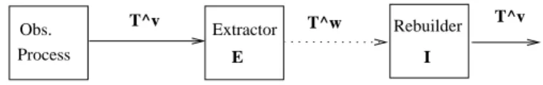
Process

Obs. T^v Extractor T^w Rebuilder T^v

E I

Figure 1: Extraction, Reconstruction, Faithfulness Property

trace T =< s0, en> (finite or infinite, here of size n ≥ t) is a partial trace Ut=< s0, et> which

corresponds to the t first events of T , with an initial state at the beginning. T may contain any prefixes of its elements.

A trace can be decomposed into segments containing trace events only, except prefixes which start with a state. An associative operator of concatenation will be used to denote sequences concatenations (denoted ++). It will be omitted if there is no ambiguity. The neutral element is [] (empty sequence). A segment (or prefix) of size 0 is either an empty sequence or a state.

Traces are used to represent the evolution of systems by describing the evolution of their state. A state of the system is described by a given finite set of parameters and a state corresponds to a set of values of parameters. Such states will be said virtual as they correspond to states of the observed system, but they are not actually traced. We will thus distinguish between actual and virtual traces.

• the actual traces (Tw_{) are a way to observe the evolution of a system by generating traces.}

The events of an actual trace have the form e = (a) where a is an actual state described by a set of attributes values. An actual states is described by a finite set of attributes. Actual traces corresponds to sequences of events produced by a tracer of an observed system. They usually encode virtual states changes in a synthetic manner.

• the virtual traces (Tv_{) corresponds to the sequence of the virtual states such that for each}

transition in the system between two virtual states, it corresponds an actual trace event. The virtual trace events have the form e = (r, s) where r is a type of action associated with a state transition and s, called virtual state, the new state reached by the transition and described by a set of parameters. Virtual traces correspond to sequences of virtual states of the observed system which produced the actual trace, together with the kind of action which produced the virtual state transition.

The correspondence between both kinds of traces is specified by two functions E : Tv_{→ T}w

and I : Tw _{→ T}v_{, respectively the extraction and the reconstruction function, as illustrated by}

the figure1.

The idea is that the actual generated trace contains as much information as possible in such way that the virtual trace can be reconstructed from the actual one. In other words, the extraction is done without loss of information. Such a property of the traces is called faithfulness and, if we denote Idv (resp. Idw) the identity between virtual traces (resp. actual traces), it

states that E ◦ I = Idv (composition) or E = I−1, and I ◦ E = Idw (or I = E−1).

Finally, each trace event is numbered by a chrono, which is an integer incremented by 1 at each new event. It will be ignored in formal presentations, but will be used as a unique identifier of the trace events in the implementations.

2.2

Components in Trace Design

When designing a trace, several components must be taken into consideration. They are depicted in the Figure2.

query Process Obs. T^v Full T^w Full T^v Partial Partial T^w Analyser Driver Extractor Rebuilder E I

Figure 2: Components in Trace Design

1. The observed process whose behavior is modeled by a virtual trace (sequence of successive virtual states) Tv_.

2. An extractor component which encodes the virtual trace into the actual one Tw_{. This}

component corresponds in practice to the tracer formalized by the extraction function E. 3. The driver which realizes the actual trace filtering according to some trace query. In this

report we limit its role to select a subtrace of the so called full trace.

4. The rebuilder which may reconstruct from a full or partial actual trace a full or partial virtual trace. This is possible only if there is no loss of information (faithfulness property). The rebuilder is formalized by the reconstruction function I.

5. The analyzer, which corresponds to some debugging tool or particular application, working with the full trace or a partial one.

Notice that in practice the three first components may be interleaved in the sense that for a given query the driver may select directly a subset of the virtual trace, thus avoiding to extract and encode a full actual trace before selecting a subtrace.

In this report we focus on three components (observed process, extractor and rebuilder) and a property. Their description consists in a faithful observational semantics.

2.3

Observational Semantics (OS)

The evolution of a system defined by its virtual traces and the production of the corresponding actual trace can be described by a so called Observational Semantics as follows. More general definitions can be found in [7].

Definition 1 (Observational Semantics) An observational semantics consists of < S, R, A, T, E, I, S0>,

where

• S: domain of virtual states, a subset of the Cartesian product of domains of parameters. • R: finite set of action types, set of identifiers labeling the transitions.

• A: domain of actual states, a subset of the Cartesian product of domains of attributes. • T r: state transition function1

T r : R × S → S, characterized as T r(ri, si−1) = si, where

(si−1, si) is the ith transition starting from an initial state s0, and labeled by ri.

• El: local trace extraction function El: S × R × S × Tw→ A, which is defined for all r, s, s′

such that T r(r, s) = s′

and characterized as

El(si−1, ri, si, Ti−1w ) = ai, where ai is the ith actual trace event generated after the initial

state s0. In this definition the extraction may use all information accumulated in the already

generated actual trace Tw i−1.

• Il: local trace reconstruction function Il: S×Tw→ R×S is characterized as Il(si−1, Tiw) =

(ri, si). The extraction function is “local” if it uses a terminal bounded subsequence of Tiw.

Here it will use the last actual trace event only ai2 (Tiw= Ti−1w ai).

• S0⊆ S, set of initial states.

The local extraction and reconstruction functions can be extended to obtain the functions E (resp. I) between sets of virtual and actual traces, as follows:

E(Tv

n) = s0El(s0, r1, s1, T0w)...El(si−1, ri, si, Ti−1w )...El(sn−1, rn, sn, Tn−1w ) = Tnw, as El(si−1, ri, si, Ti−1w ) =

ai and Tiw= s0a1...ai. And

I(Tw

n) = s0Il(s0, T1w)...Il(si−1, Tiw)...Il(sn−1, Tnw) with Il(si−1, Tiw) = (ri, si).

The Observational Semantics is faithful if E and I satisfy the faithfulness property, i.e. if ∀Tv_{, T}w_{f inite, E(T}v_{) = T}w_{∧ I(T}w_{) = T}v_.

Exemple 1

The figure3illustrates the following simple automaton (arrows are labeled by type of actions). • S = {s0, s1, s2},

• R = {a, b}, • A = {a, b},

• ∀s, T (b, s) = s1, T (a, s1) = s2,

• El(s, r, s′) = r (the generated actual trace is not used),

• ∀s, Il(s, b) = (b, s1), Il(s1, a) = (a, s2) (the last actual trace event only is used),

• S0= {s0}.

The virtual traces are: s0(b, s1)+{(a, s2)(b, s1)+} ∗

. The actual traces are: s0b+(ab+) ∗ . s₁ s₂ b b b a s₀

Figure 3: Exemple1: Finite State Automaton

It is straightforward to see that this OS is faithful, using the regular expression form of the traces.

2_{In general a bounded number of element should be used, but also some forward elements like a}

i+1... For

2.4

Faithful Trace Specification

We first give a condition for an OS to be faithful. Proposition 1

Given an OS < S, R, A, T r, El, Il, S0>, E and I the extensions of El and Ilas above, if the

following condition holds: ∀r, s, s′ , a, Tw_{, T r(r, s) = s}′ ⇒ (El(s, r, s ′ , Tw_{) = a ∧ I} l(s, Twa) = (r, s ′ )), where Tw_{is a finite}

actual trace generated by successive applications of the transition function T r from an initial state s0until an ultimate state s,

then the OS is faithful, i.e. ∀Tv_{, T}w_{f inite, E(T}v_{) = T}w_{∧ I(T}w_{) = T}v_{, where T}v _{is a virtual}

trace corresponding to successive applications of the transition function T r from an initial state s0 until an ultimate state s.

Proof 1 The proof is by induction on the size of the traces. By definition with each new transition actual and virtual traces are increased by one event only. Initially: (traces of size 0) E(s0) = s0∧ I(s0) = s0.

Let us assume the property holds for a trace of size n: (1) E(Tv

n) = Tnw∧ I(Tnw) = Tnv (2).

(1) means, according to the definition of E, that Tw

n is the actual trace generated by n

suc-cessive applications of T r function from a state s0until some ultimate state sn by using the local

extraction function El at each step.

(2) means, according to the definition of I, that Tv

n is the virtual trace reconstructed from the

actual trace Tw

n. The holding conjunction means that the reconstructed virtual trace is the same

as the one used to produce the actual one, therefore I(Tw

n) ends in a state sn, the same as for

Tv n.

One shows that (++ concatenation and list constructor are omitted for singletons) (1’) E(Tv

n+1) = Tn+1w ∧ I(Tn+1w ) = Tn+1v (2’) holds.

Assume that the ultimate state reached by Tv

n is sn. Then by definition (if sn is not a final

state), ∃rn+1sn+1, T r(rn+1, sn, sn+1) holds, hence: Tn+1v = Tnv(rn+1, sn+1), and, by definition

Tw

n+1= Tnwan+1.

(1’) holds: E(Tv

n+1) = E(Tnv(rn+1, sn+1)) = TnwEl(sn, rn+1, sn+1, Tnw) = Tnwan+1= Tn+1w , by hypothesis (1)

and where the last argument of El, Tnw, is the actual trace resulting from E(Tnv).

(2’) holds: I(Tw

n+1) = I(Tnwan+1) = TnvIl(sn, Tnw) = Tnv(rn+1, sn+1) = Tn+1v , by hypothesis (2) and the

definition of Il.

The proposition 1 shows how to design a faithful observational semantics: by specifying together the local extraction and reconstruction functions, verifying at each step defined by the transition function that the generated trace allows to reconstruct the same reached state as the one specified by the transition function.

This results can be extended to actual subtraces (defined as traces obtained by considering a subset of attributes of the actual traces), provided that there are sufficiently many attributes in the subtrace to recompute parameters (then the corresponding virtual subtrace is a virtual trace with a subset of parameters)3_.

This is illustrated in the figure2. A query applied to the actual trace selects a partial actual trace in such a way that the resulting partial trace can be reconstructed as a partial virtual trace

3_{This implies some restrictions on the kind of queries (in case of dependencies between parameters or}

(the one from which the partial actual trace could be extracted). In practice, the generic trace specification consists of an operational semantics corresponding to some abstract level of process observation, instrumented to produce an actual trace. The level of description (granularity of the events) should be chosen in such a way that this abstract operational semantics can be abstracted from each particular semantics of each process of the family. Symmetrically, it is requested that the abstract operational semantics can be “implemented” in each process of the family.

The faithfulness property of the observational semantics guarantees that the generic actual trace preserves the whole information concerning the process behavior, in such a way that all desirable properties of the semantics can be studied just by looking at the trace.

3

Generic Trace for CHR

In this section we introduce the generic trace proposed for CHR∨

. It is based on the refined Theoretical Operational Semantics for CHR, ω∨

r, as defined in [5].

Such semantic is declarative enough to cover most of the CHR implementations. It is the case for ECLiPSe Prolog [2] and SWI-Prolog [19] whose operational semantics can be viewed as a refinement of ω∨

r (conversely ω ∨

r can be viewed as an abstraction of the semantics of these

implementations).

3.1

Introducing CHR

Constraint Handling Rules emerges in the context of Constraint Logic Programming (CLP) as a language for describing Constraint Solvers. In CLP, a problem is stated as a set of constraints, a set of predicates and a set of logical rules. Problems in CLP are generally solved by the interaction of a logical inference engine and constraint solving components. The logical rules (written in a host language) are interpreted by the logical inference engine and the constraint solving tasks are delegated to the constraint solvers. We borrow from [17] some elements of presentation.

The following rule base handles the less-than-or-equal problem:

a n t i s y m m e t r y @ leq( X , Y ) , leq ( Y , X ) <=> X = Y . reflexivi t y @ leq( X , X ) <=> true.

idempoten c e @ leq( X , Y ) \ leq ( X , Y ) <=> true. t r a n s i t i v i t y @ leq( X , Y ) , leq ( Y , Z ) ==> leq ( X , Z ) .

This CHR program specifies how leq simplifies and propagates as a constraint. The rules implement reflexivity, antisymmetry, idempotence and transitivity in a straightforward way. The ref lexivity rule states that leq(X, Y ) simplifies to true, provided it is the case that X = Y . This test forms the (optional) guard of a rule, a precondition on the applicability of the rule. Hence, whenever we see a constraint of the form leq(X, X) we can simplify it to true.

The antisymmetry rule means that if we find leq(X, Y ) as well as leq(Y, X) in the constraint store, we can replace it by the logically equivalent X = Y . Note the different use of X = Y in the two rules: in the ref lexivity rule the equality is a precondition (test) on the rule, while in the antisymmetry rule it is enforced when the rule fires. (The reflexivity rule could also have been written as ref lexivity@leq(X, X) <=> true.)

The rules ref lexivity and antisymmetry are simplification rules. In such rules, the constraint found are removed when the rule applies and fires. The rule idempotence is a simpagation rule,

only the constraint in the right part of the head will be removed. The rule says that if we find leq(X, Y ) and another leq(X, Y ) in the constraint store, we can remove one.

Finally, the transitivity rule states that the conjunction leq(X, Y ), leq(Y, Z) implies leq(X, Z). Operationally, we add leq(X, Z) as (redundant) constraint. without removing the constraints leq(X, Y ), leq(Y, Z). This kind of rule is called propagation rule.

The CHR rules are interpreted by a CHR inference engine by rewriting the initial set of constraints by the iterative application of the rules. Its extension with disjunctive bodies, CHR∨

boosts its expressiveness power, turning it into a general programming language (with no need of an host language).

Summarizing, there are three kinds of rules in CHR as in CHR∨_{: simplification, propagation}

and simpagation.

The simpagation rules are the most general category of rules and they have the following form r@Hk\Hr ⇔ G|B., where r is an identifier for the rule, Hr and Hk are the heads of the

rule (in the following they will be denoted respectively as keep and remove), G is the guard, and B is the body. If the guard is true, it can be omitted.

The operational semantics of such rule is that if Hk and Hrare found in the constraint store

and the guard G is entailed by it, the constraints in Hr should be removed and the constraints

in the body B should be added to the constraint store. If Hk is empty, this rule is called a

Simplification Rule, and this part of the rule is omitted. On the other side, if Hr is empty, this

rule is called a Propagation Rule. In this case, the second part of the head of the rule is omitted and the ⇔ is replaced by the symbol ⇒.

In CHR∨

, we distinguish two kinds of constraints: Rule defined constraints (RDC), which are declared in the current program and defined by CHR rules, and built-in constraints (BIC), which are predefined in the host language or imported CHR constraints from some other module. Furthermore, in CHR∨

, bodies may contain disjunctions. Exemple 2 The following CHR∨

rule defines the append(X,Y,Z) constraint: r1 @ append(X,Y,Z) <=> (X = [], Z = Y);

(X = [H|L1], Z = [H|L2], append(L1,Y,L2)).

In this rule, Z is a list composed by the elements of the list X followed by the elements of the list Y. If append(X,Y,Z) holds, we have two options: (i) X=[] and, therefore, Z=Y; or (ii) X is a list in the form [H|L1], and thus, Z is composed by H followed by L1 and then followed by the elements in Y.

We illustrate the CHR∨

solver behavior, by showing the effect of successive applications of the CHR∨

rules on the constraint store. Let us suppose the initial state of the constraint store is append([1], [2], Z). The actual execution of this rule base is represented by the following set of transitions. The notation hG0i ; . . . ; hGni represents the alternative stores. The transition 7→r₁

represents the application of r1 and the transition 7→∗ the removal of failed stores. Notice that

from the final state we can conclude Z = [1, 2]:

happend([1], [2], Z)i 7→r

1

h[1] = [], Z = [2]i ; h[1] = [1|[]], Z = [1|L2], append([], [2], L2)i 7→∗

h[1] = [1|[]], Z = [1|L2], append([], [2], L2)i 7→r

1

[] = [H|L1], L2 = [H|L2′_{], append(L1, [2], L2}′₎₎ 7→∗ h[1] = [1|[]], Z = [1|L2], [] = [], L2 = [2]i

3.2

Operational Semantics ω

r semantics given here is adapted from [9].

We define CT as the constraint theory which defines the semantic of the built-in constraints and thus models the internal solver which is in charge of handling them. We assume it supports at least the equality built-in. We use [H|T ] to indicate the first (H) and the remaining (T ) terms in a list or stack, + for pushing elements into stack (there may be several pushed elements represented as a list), ++ for sequence concatenation and [] for empty sequences. We use the notation {a0, . . . , an} for both bags and sets. Bags are sets which allow repeats. We use ∪ for set

union and ⊎ for bag union, {} to represent both the empty bag and the empty set, and E − E′

to remove all occurrences of elements of E′

from E. The identified constraints have the form c#i, where c is a user-defined constraint and i a natural number. They differentiate among copies of the same constraint in a bag. We also use the functions chr(c#i) = c and id(c#i) = i with their natural extension to lists of constraints and of identifiers.

A CHR program is a sequence of rules, and the head and body of a rule are considered sequences of atomic constraints. A number is associated with every atomic head constraint, called the occurrence. Head constraints are numbered per functor, starting from 1,in top-down order from the first rule to the last rule, and from left to right. However, removed head constraints in a simpagation rule are numbered before kept head constraints. This numbers will be used to show in witch position the active constraint is (the j indicator).

An execution state E is a tuple hA, S, B, T in, where

• A is the execution stack;

• S is the UDCS (User Defined Constraint Store), a bag of identified user defined constraints; • B is the BICS (Built-in Constraint Store), a conjunction of constraints;

• T is the Propagation History, a set of sequences for each recording the identities of the user-defined constraints which fired a rule;

• n is the next free natural used to number an identified constraint.

Current alternatives are denoted as ordered sequence of execution states, L = [E1, E2, ...En]

where E1 is the active execution state and [E2, ..., En] the remaining alternatives.

The initial configuration is represented by L0 = [hA, {}, true, {}i₁]. The top of execution

stack A is a “goal” constraint (the one corresponding to the initial goal of the program) that will be processed.The transitions are applied non-deterministically until no transition is applicable anymore.

The formal description of the transitions is done in the form of rules: for each type of action r ∈ R there is a rule of the form r s 7→ s′_{, such that T r(r, s) = s}′_.

Solve+Wake [h[c|A], S, B, T in|L] 7→ [hA

′_{+ A, S, c ∧ B, T i}

n|L], where c is built-in

and A′ _{= wakeup(S, c, B) where wakeup is a function that implements the}

wake-up policy[9] whose result is a list of constraints of S woken by adding c to B.

Activate [h[c|A], S, B, T in|L] 7→ [h[c#n : 1|A], c ⊎ S, B, T in+1|L], where c is

user-defined constraint.

Reactivate [h[c#i|A], S, B, T in|L] 7→ [h[c#n : 1|A], S, B, T in|L], where c is

user-defined constraint.

Apply.1 [h[c#i : j|A], H1⊎ H2⊎ S, B, T in|L] 7→ [h[c#i : j|A], H1⊎ H2⊎ S, B, T in|L]

where the jth

occurrence of a constraint with same functor as c exists in

the head of a fresh variant of a rule r@H′

1\H2′ ⇔ g|C and a matching

substitution modulo B, ea

, such that chr(H1) = e(H1′), chr(H2) = e(H2′) and

{(r, id(H1)++id(H2))} /∈ T .

Apply.2 [h[c#i : j|A], H1⊎ H2⊎ S, B, T in|L] 7→ [hC + H + A, H1⊎ S, e ∧ B, T ′_i

n|L]

where the jth

occurrence of a constraint with same functor as c exists in

the head of a fresh variant of a rule r@H′

1\H2′ ⇔ g|C and a matching

substitution moduloB, ea

, such that chr(H1) = e(H1′), chr(H2) = e(H2′)

and {(r, id(H1)++id(H2))} /∈ T and CT |= ∃(B) ∧ ∀B ⊃ ∃(e ∧ g) and

T′ _{= T ∪ {(r, id(H}

1)++id(H2))}, and H = c#i : j if c is in H1, H = [] if c is

in H2, and c ∈ H1∨H2.

Drop [h[c#i : j|A], S, B, T in|L] 7→ [hA, S, B, T in|L], where there is no occurrence j

for c in the program.

Default [h[c#i : j|A], S, B, T in|L] 7→ [h[c#i : j + 1|A], S, B, T in|L], if no other

tran-sition is possible in the current state.

Split [h[c1∨ ... ∨ cm|A], S, B, T in|L] 7→ [σ1, ..., σm|L], where σi = h[ci|A], S, B, T in,

for 1 ≤ i ≤ m. This transition implements depth-first, other search strategies can be implemented by easily changing this definition.

Fail [E |L] 7→ L, This transition is called automatically if E is a failed state. By definition a failed state occurs when the Built-in store is false.

a

The matching substitution will record all Equalities in the Built-in Store

This semantics is adapted from [9], it differs mainly by two additional type of actions: Ap-ply.1 (Apply.2 corresponds to the original Apply rule) and Fail. ApAp-ply.1 corresponds to an attempt of using a CHR rule and will be applied only once for each j, H1, H2 occurrence. If the transition Apply.2 is applied, there was an application of Apply.1 for the same occurrence j, but the converse does not hold. The Fail case corresponds to a failed computation. In this case, other alternatives are explored.

3.3

Generic Trace

We introduce here the generic actual trace of CHR∨

informally. Each transition in the ω∨ r

semantics should generate an actual trace event. Here are the expected types of actions together with the other possible attributes. There are two categories of attributes: those coding the virtual states which may serve for the reconstruction, some others may bring useful information for potential applications.

Each transition corresponding to the type of action r generates an actual trace event whose first attribute characterizes r uniquely. A subset of the attributes only is attached to a specific type of event. Attributes are as follows:

• Port, or Event Name: p. It belongs to

{W ake, ActivateRDC, ReactivateRDC, T ryRule, ApplyRule, Drop, Def ault, Split, F ail}.

There is an obvious bijection between R (the set of type of actions) of the OS and this set of event names. It belongs to all events and is always the first attribute.

• Constraint instance of some type w where the constraint is a term c before the first activation, or c#i : j in the other cases, where i and j are integers. A constraint will be represented by a list of form [p, t1, t2, ..., tm] or [p, t1, t2, ..., tm, i, j]. w is cons in the former

case and cinst in the later.

• List of constraints instances of some type w: w-lc. It may be a list of terms or a list of the form [w, [[c1], ..., [cm]]], each element represented by a list as above. w is the kind

of constraints. It may be woken, addrdc, addbic, keep, remove or guard constraints, or a matching substitution match, represented by a list of equations.

• Reference to a previous trace event: ref, where ref has the form @i and i is an integer identifying a previous actual trace event (a previous chrono).

• Rule name: r@, where r@ is the name of a rule in the source program.

• State number: n. An integer corresponding to the parameter numbering a solver virtual state. It belongs to all events and is always the last attribute.

This is formalized in the following tables. The first table is a context free syntax of the generic trace. Terminals are between brackets. Non terminals corresponding to attributes are names of attributes. Optional items are between square brackets (those which are not in terminals), options are separated by vertical bars. Brackets after ∈ denote a set (to avoid multiplicity of rules).

Gen. traceT ::= Ev_1...Ev_m, m ≥ 0

Ev ::= {GT: [} Chrono {,} Port [Other] Spec_Attr {,} StateNumber {]}

Chrono ::= {integer}

Port ∈ { W ake, ActivateRDC, RectivateRDC, T ryRule, ApplyRule, Drop, Def ault, Split, F ail }

Other ::= Ref | RuleName | Indice | CT | CTIJ Ref ::= {, @ integer}

RuleName ::= {, identifier @} Indice ::= {, integer}

Spec_Attr ::= ǫ | {,} SpecAttr Spec_Attr SpecAttr ::= {[} Attr ListCT {]}

Attr ∈ { Woken, Addrdc, Addbic, Keep, Remove, Guard, Match }

ListCT ::= ǫ | {,} (CT | CTIJ) ListCT) CT ::= {[ predicate, t_1, ..., t_n ]} CTIJ ::= {[ predicate, t_1, ..., t_n, i, j ]} StateNumber ::= {integer}

The following table gives the list of the attributes other than Chrono, Port and StateNumber for each type of event. The firts item is the transition name (∈ R), the second item the corre-sponding port (value of the attribute Port) and the last item is the list of attributes.

r ∈ R Port Specific Attributes Solve+Wake W ake Cons, Woken Activate ActivateRDC Cinst Reactivate ReactivateRDC Cinst, Ref

Apply.1 T ryRule RuleName, Cinst, Keep, Remove, Guard Apply.2 ApplyRule Ref, Addrdc, Addbic, Remove, Match, Cinst Drop Drop Cinst

Default Def ault Index Split Split Ref Fail F ail Ref

Table 2: Specific Attributes for each type of event (except chrono and state number) The following lists all attributes (specific or other) for each actual trace event corresponding to some type of action. All examples4

are extracted from a generic trace of the section6.3. • Solve+Wake (port W ake): a built-in constraint (BIC) is solicited and some constraints

are woken

2 attributes (total 5):

– Cons: the built-in constraints being “executed”.

– Woken: the (possibly empty) list of the constraints woken by the wake-up policy. Example: GT: [61,Wake,[=,C1,a0],[woken,[[node,r1,C1,359]]],360]

• Activate (port ActivateRDC): activate a Rule Defined Constraint (RDC) getting the RDC c#i : j from the top of the execution stack and activating it.

1 attribute (total 4):

– Cinst: the user defined constraint which is “introduced” and “executed”. The attribute value is the created instance of this constraint.

Example: GT: [3,ActivateRDC,[edge,r1,r9,332],333]

• Reactivate (port ReactivateRDC): Activate a Rule defined constraint with justification 2 attributes (total 5):

– Cinst: the user-defined constraints instance being “re-executed”, which became active. – Ref: a reference to the Solve+Wake event where this constraint has been woken

(form of justification).

Example: GT:[62,Reactivate,[node,r1,a0,359],@61,360]

• Apply.1 (port T ryRule): attempt to apply a Rule; it may be followed by an Apply.2 event in case of successful application, or another event in case it cannot by applied.

5 attributes (total 8):

4_{The Prototype does not generate the j index of the constraint, therefore there isn’t any example with this}

– RuleName: the name of the tried rule in the source code.

– Cinst: the active user-defined constraint instance (the one at the top of the execution stack).

– Keep: the keep constraints of the store used to match the head of the tried rule. – Remove: the remove constraints of the store used to match the head of the tried rule. – Guard: the guard constraints of the tried rule (as in the source program). This

infor-mation may be useful in case of failure.

Example: GT: [102,T ryRule,wrong@,[node,r5,a0,375], [keep,[[node,r4,a0,371], [edge,r4,r5,340], [node,r5,a0,375]]], [remove,[]],[guard,[[=,a0,a0]]],376] • Apply.2 (port ApplyRule): applying the rule with success (true guard)

7 attributes (total 10):

– Ref: a refence to the previous Apply.1 event where the name of the applied rule, the active constraint and some other information can be found.

– Addrdc: the user-defined constraints instances of the body of the applied rule, pushed on the stack.

– Addbic: the built-in constraints instances of the body of the applied rule, pushed on the stack.

– Keep: the keep constraints of the store used to match the head of the tried rule. – Remove: the remove constraints of the store used to match the head of the tried rule. – Match: the successful matching equations (a way to give the current substitution). – Cinst: the active user-defined constraint instance (the one at the top of the execution

stack).

Example: GT: [103,ApplyRule,@102,[addrdc],[addbic,[fail,fail]], [keep,[[node,r4,a0,371], [edge,r4,r5,340], [node,r5,a0,375]]], [remove,[]],[match,[edge(Ri,Rj)=node(,r4,a0)], [node(Ri,Ci)=edge(,r4,r5)], [node(Rj,Cj)=node(,r5,a0)]], [node,r5,a0,375],376] • Drop (port Drop): drop a constraint. The currently active constraint c#i : j is removed

from the stack. There is no more occurrences j for c in the program. 1 attribute (total 4):

– Cinst: the constraint which is popped from the execution stack. Example: GT: [4,Drop,[edge,r1,r9,332],333]

• Default (port Def ault): The occurrence index j of the active constraint c#i : j is incre-mented (proceed to the next occurrence of the constraint instances in the program). There is no more occurrences j for c in the program.

2 attributes (total 5):

– Cinst: the last used constraint occurrence.

– Index: The occurrence Index j is incremented (proceed to the next occurrence of the constraint instances in the program.

Example: GT: [28, Def ault, [node, r7, r, 5, 386], 6, 388]5

5_{It’s a hand-made example. Although, It’s not difficult to compute how many Default transitions was applied}

• Split (port Split): create a disjunction. Occurs when a rule is disjunctive. 1 attribute (total 4):

– Ref: a reference to the most recent Apply.2 event with the rule whose body contains the disjunction.

Example: GT: [60,Split,@59,360]

• Fail (port F ail): the referred rule application fails. It Occurs when the Built-In store has been tested false.

1 attribute (total 4):

– Ref: a reference to the most recent failed Apply.2 event. Example: GT: [104,F ail,@103,376]

All the variables which occur in the initial goal will keep their original name in all their occurrences in the generic trace. Each actual trace event has a unique identifier, called the chrono, which is an integer incremented by 1 at each new event.

The formal definition of trace generation will be given in section4.1.

4

Observational Semantics of CHR

(OS-CHR

)

We specify the observational semantics of CHR∨_{, OS-CHR}∨_{, on the top of the operational}

semantics of section3.2, by specifying the transition function and the local functions of extraction El and of reconstruction Il. The resulting OS, called OS-CHR∨, is faithful by construction (by

property1).

According to the definition1, the observational semantics consists of < S, R, A, T r, El, Il, S0>.

The definition of the transition function T r is given by the operational semantics. The definitions of El, Il are given in the next two sections. The others elements are as follows.

• S: domain of virtual states. It the set of configurations defined as a list of execution states, where an execution state E is defined by the hA, S, B, T in as described in the section3.2.

• R: finite set of action types: {Solve+Wake, Activate, Reactivate, Apply.1, Apply.2, Drop, Default, Split, Fail}

• A: domain of actual states: each state consists of a tuple of values of a subset of the attributes. All attributes are defined in the section3.3.

• S0⊆ S, set of initial states, specified below.

In this presentations the chrono is omitted.

4.1

OS-CHR

: Extraction (T r, E

)

This description is based on the transitions as described in the table 3.2. Each item corresponds to a type of action and it specifies the new generated actual trace event, using the previous state, the reaches state and the previously generated actual trace. The current generated actual trace is denoted N , an ordered sequence of the trace events. It has the form, for each type of action r and transition T r(r, s) = s′_{: E}

r s, N 7→ s′

, N ++a The initial configuration will be represented as L0= [hA, {}, true, {}i1], N = []

Solve+Wake

[h[c|A], S, B, T in|L], N 7→ [hA′+ A, S, c ∧ B, T in|L],

N ++[W ake, c, wakeup(S, c, B), n], where SolveCond.

Activate [h[c|A], S, B, T in|L], N 7→ [h[c#n : 1|A], c ⊎ S, B, T in+1|L],

N ++[ActivateRDC, c, n], where c is a rule-defined constraint

Reactivate [h[c#i|A], S, B, T in|L], N 7→ [h[c#n : 1|A], {c#n} ⊎ S, B, T in|L],

N ++[ReactivateRDC, c, wake(c, N )], where CondReac (see below)

Apply.1 [h[c#i : j|A], H1⊎ H2⊎ S, B, T in|L], N 7→

[h[c#i : j|A], H1⊎ H2⊎ S, B, T in|L], N ++[T ryRule, r, c#i : j, H1, H2, g, n]

where CondApp1 (see below).

Apply.2 [h[c#i : j|A], H1⊎ H2⊎ S, B, T in|L], N 7→

[hC + [H|A], H1⊎ S, e ∧ B, T′in|L],

N ++[ApplyRule, tryRule(N ), addRDCs(C), addBICs(C), H1, H2, e, H, n]

where CondApp2 (see below).

Drop [h[c#i : j|A], S, B, T in|L], N 7→ [hA, S, B, T in|L], N ++[Drop, c#i : j, n].

Where c is an active constraint.

Default [h[c#i : j|A], S, B, T in|L], N 7→ [h[c#i : j + 1|A], S, B, T in|L], N ++

[Def ault, c#i : j, j + 1, n].

Split [h[c1∨ ... ∨ cm|A], S, B, T i_n|L], N 7→ [σ1, ..., σm|L], N ++[Split, rule(N ), n],

where CondSplit (see below).

Fail [E |L], N 7→ L, N ++[F ail, rule(N ), n], where CondF ail (see below).

The conditions appearing in our observation semantics are defined as follows: SolveCond: c is built-in, and A′

= wakeup(S, c, B) defines which CHR constraints of S are woken by adding the constraint c to the built-in store B.

CondReac: the function wake : Constraint, T race 7→ W ake is responsible for selecting the Wake event that justifies the Reactivate.

CondApp1: where the jth _{occurrence of a constraint with same functor as c exists in the}

head of a fresh variant of a rule r@H′ 1\H

′

2 ⇔ g|C and a matching substitution e, such that

chr(H1) = e(H ′

1), chr(H2) = e(H ′

2) and {(r, id(H1)++id(H2))} /∈ T .

CondApp2: C is the body of the rule r@H′ 1\H

′

2 ⇔ g|C. The tryRule : T race 7→ T ryRule

will retrieve the TryRule event generated by Apply.1. It will search for the event in the trace log, normally the event TryRule will be one step back. addRDCs : Body 7→ Sequence(RDC) will select only the RDCs on the body; the function addBICs : Body 7→ Sequence(BIC) will select the BICs on the body. Same conditions of Apply.1 plus CT |= ∃(B) ∧ ∀B ⊃ ∃(e ∧ g) , T′

= T ∪ {(r, id(H1)++id(H2))}, and H = c#i : j if c is in H1, H = [] if c is in H2, and

c ∈ H1∨H2.

CondSplit: where σi= h[Ai|A], S, B, T in, for 1 ≤ i ≤ m, and rule : T race 7→ ApplyRule is a

function that will retrieve the cause of the split, a disjunctive rule.

CondF ail: n is the numbering of the failed state E, and rule(N ) is a function that will retrieve the cause of the failure.

4.2

OS-CHR

: Reconstruction (I

)

We show here, by specifying a local reconstruction function Il, that the observationa semantics

is faithful, i.e. that the extracted (actual) generic trace contains all information needed to reconstruct the original virtual trace (the trace semantics equivalente to the given operational semantics).

The local reconstruction function takes a current state s and the generated actual trace including the last generated event a, N ++a; it identifies the type of action r and produces the new virtual state s′

. It has the form, for each type of action r: Il(s, N a) = (r, s ′ ), which will be represented by a rule: r s, N ++a 7→ s′ with a = [r|a′ ].

The initial configuration will be represented as L0= [hA, {}, true, {}i₁], N = []

For each item corresponding to a type of action, the reconstructed state s′ _{is the same as the}

new state obtained by the corresponding transition T r(r, s) = s′ _{as described in the table 3.2.}

This constitutes the proof of faithfulness of OS-CHR∨_{, by property1.}

The conditions consists of an optional condition part and a computation part. They are just used here to express computations.

Solve+Wake

[hA, S, B, T in|L], N ++[W ake, c, C, n

′_{] 7→ [hC + A}′_{, S, c ∧ B, T i}

n′|L], if

SolveCond.

Activate [hA, S, B, T in|L], N ++[ActivateRDC, c, n

′_{] 7→}

[h[c#n′_{: 1|A}′_{], c ⊎ S, B, T i}

n+1|L], if ActiCond.

Reactivate [hA, S, B, T in|L], N ++[ReactivateRDC, c#i, wakeEvent, n′] 7→

[h[c#n′_{: 1|A}′_{], {c#n}′_{} ⊎ S, B, T i}

n′|L], if CondReac.

Apply.1 [hA, S, B, T in|L], N ++[T ryRule, r, c#i : j, H1, H2, g, n′] 7→

[h[c#i : j|A′_{], H}

1⊎ H2⊎ S′, B, T in|L], if CondApp1.

Apply.2 [hA, S, B, T in|L], N ++[ApplyRule, r, RDCs, BICs, H1, H2, e, H, n′] 7→

[hC + A, H1⊎ S′, e ∧ B, T′in|L], if CondApp2.

Drop [hA, S, B, T in|L], N ++[Drop, c#i : j, n

′_{] 7→ [hA}′_{, S, B, T i}

n′|L], if DropCond.

Default [hA, S, B, T in|L], N ++[Def ault, c#i : j, j

′_{, n}′_{] 7→}

[h[c#i : j′_|A′_{], S, B, T i}

n′|L], if Def Cond.

Split [hA, S, B, T in|L], N ++[Split, r, n′] 7→ [σ1, ..., σm|L′], if CondSplit.

Fail [hA, S, B, T in|L], N ++[F ail, r, n

′_{] 7→ L, if CondF ail.} SolveCond: A = [c|A′ ] ∧ n = n′ ∧ C = wakeup(S, c, B). ActiCond: A = [c|A′ ] ∧ n = n′ . CondReac: A = [c#i|A′ ] ∧ wakeEvent = wake(c, N ) ∧ n = n′ . CondApp1: A = [c#i : j|A′

] ∧ S = H1⊎ H2⊎ S ′

∧ n′

= n. CondApp2: A = H +A′

, C is the body of the rule hr@H′ 1\H ′ 2⇔ g|Ci∧S = H1⊎H2⊎S ′ ∧T′ = T ∪ {(r, id(H1) + id(H2))} ∧ n ′

c ∈ H1∨H2..

DropCond: A = [c#i : j|A′

] ∧ n′

= n. Def Cond: A = [c#i : j|A′

] ∧ j′

= j + 1 ∧ n′

= n.

CondSplit: A = h[A1∨ ... ∨ Am|A′], S, B, T i_n∧σi= h[Ai|A], S, B, T i_n, for 1 ≤ i ≤ m∧n′= n.

CondF ail: n′

= n.

Notice that the local reconstruction function does not use the full generated trace, but the last actual trace event only. This guarantees a better efficiency for analysis. However this is obtained at the cost of including specific details into the generic trace. For example the attribute n (state indicator) could be retrieved from the current virtual state; the fact to have it in the current actual trace event avoids some computation.

5

Prototyping the Operational Semantics of CHR

The objective of building a prototype of the operational semantics described in the section3.2is to produce tests of trace generation, in order to improve the quality of the design. In fact there is no way to prove that the specification given in an algebraic style, with some implicit or informal parts, is sound. Indeed the simple fact to implement in Prolog an executable specification with which it is possible to simulate the extraction of the generic trace is a step towards a better quality of the proposed formal specification.

The SWI-Prolog implementation of the operational semantics of CHR∨

is built with the feature to produce the generic trace. The following subsections illustrate the architecture of the proposed implementation. The full program is given in the annexe.

5.1

CHR

Syntax and Rule Compilation

Listing 1: CHR∨ Syntax :− op( 1 1 0 0 , xfx , \ ) . :− op( 1 1 8 0 , xfx ,==>) . :− op( 1 1 8 0 , xfx ,<=>) . :− op( 1 1 9 0 , xfy , @ ) . The CHR∨

Syntax is represented Prolog infixed operators as presented in Listing1. This syntax accepts CHR∨

rules like in the following CHR program:

t r a n s i t i v i t y @ leq( vX , vY ) , leq ( vY , vZ ) ==> leq ( vX , vZ ) . idempoten c y @ leq( vX , vY ) / leq ( vX , vY ) <==> true. a n t i s y m m e t r y @ leq( vX , vY ) , leq ( vY , vX ) <==> vX=vY .

However, the CHR∨

Operational Semantics does not search rules individually. It searches for the i-th occurrence of some constraint operator in program. In order to provide the appropriate information, the CHR∨

implementation generates a compiled version of this CHR∨

program as presented below:

rule( leq , 1 , transitivity , [ vX , vY ] ,

[ ] , [ leq ( vX , vY ) , leq ( vY , vZ ) ] , [ ] , [ leq ( vX , vZ ) ] ) . rule( leq , 2 , transitivity , [ vY , vZ ] ,

[ ] , [ leq ( vX , vY ) , leq ( vY , vZ ) ) ] , [ ] , [ leq ( vX , vZ ) ] ) . rule( leq , 3 , idempotency , [ vX , vY ] ,

[ leq ( vX , vY ) ] , [ leq ( vX , vY ) ] , [ ] , [true] ) . rule( leq , 4 , idempotency , [ vX , vY ] ,

[ leq ( vX , vY ) ] , [ leq ( vX , vY ) ] , [ ] , [true] ) . rule( leq , 5 , antisymmetry , [ vX , vY ] ,

[ active , leq ( vY , vX ) ] , [ ] , [ ] , [ vX=vY ] ) rule( leq , 5 , antisymmetry ,

[ vY , vX ] , [ leq ( vX , vY ) , leq ( vY , vX ) ] , [ ] , [ ] , [ vX=vY ] )

the predicate rule(Op,Ind,Rule,Args,Remove,Keep,Guard,Body) identifies the CHR∨

rule that contains the Indth occurrence of Op in its head.

5.2

Auxiliary Functions

To implement CHR∨

Operational Semantics, it was necessary to define some auxiliary functions responsible for variable management and built-ins implementation.

Variables

In the proposed CHR∨

implementation variables can be classified as local or global. Local variables are used in CHR∨

Rules and should be replaced by global variables or constants when the rule is executed. CHR∨

variables are not directly implemented using Prolog’s variables because it was desirable to give more informations about variable names to trace and the search method.

In the implementation, variable can be any Prolog’s atom. The predicates global_variable\1 and local_variable are used to decide if some term represents a global or local variable, re-spectively. In the initial implementation local variables are atoms whose first letter is “v” and the second is a upper-case letter. Global variables are terms in the form v(_) or atoms initiated with “v”, followed by a lower-case letter.

Local variables should be replaced by constants or global variables when a CHR∨

is exe-cuted. The predicate: instantiate_locals(T1,T2,Binds) replaces the local variables found in T1 by other values, producing the term T2; the argument Binds contains the performed substitutions. In T1 local variables are not replaced by a constant, the instantiable_locals predicate replaces the local variable by an undefined prolog variable. The auxiliary predicate allocate_unusedvars, instantiates these undefined variables with free global variables. Built-ins Constraint

The equality constraint (=) is the only built-in constraint implemented. The built-in memory contains a list of normalized equalities in the form:

GlobalVariable = (GlobalVariable | Constant).

To manipulate the built-in memory, two auxiliary functions are defined:

• solve_builtin(C,B1,B2,UDC1,UDC2): inserts the built-in constraint C in the built-in memory B1, producing the built-in memory B2. If the memory becomes inconsistent, the resultant memory produced is false. When the built-in constraint is inserted in memory, the User Defined Constraints Memory UDC1 is analyzed and the constraints affected by the built-in insertion are listed in UDC2.

• replace(T1,B,T2): replaces the global variables in T1 by their values (if they are defined), producing the term T2.

5.3

CHR

Operational Semantics Implementation

The CHR∨

Operational Semantics implementation is similar to the semantics proposed in Section 3.2. To illustrate this implementation, Listing2presents the Prolog implementation of the rules bf Solve+Wake and Activate.

Listing 2: Solver+Wake Rule

%S o l v e+Wake Rule

[ ( [ C | A ] , UDC , B , H , N ) | Tl ]−−>[(A2 , UDC2 , B2 , H , N ) | Tl ] :− is_builtin( C ) ,

s o l v e _ b u i l t i n( C , B , B2 , UDC , Wokeup ) , merge( Wokeup , A , A2 ) ,

remove( UDC , Wokeup , UDC2 ) . %A c t i v a t e Rule [ ( [ C | Tl ] , UDC , B , H , N ) | T ] −−−> ( [ ( [ ( C3#0) | Tl ] , [ C3 | UDC ] , B←֓ , H , N2 ) ] | T ) :− is_UDC( C ) , replace( C , B , C2 ) , C3 = C2^N , N2 i s N + 1 .

5.4

Generic Trace Extraction

To generate the generic trace in the executable operational semantics, the predicate: gentrace(Id,Data) in added. It generates a trace with the information contained in Data. The Id represents the ordering number of the generated trace. To illustrate this, Listing3contains the modified version of the rules presented in Listing2.

Listing 3: Solver+Wake Rule

%S o l v e+Wake Rule

[ ( [ C | A ] , UDC , B , H , N ) | Tl ] −−−> ( [ ( A2 , UDC2 , B2 , H , N ) | Tl ] ) ) ←֓ :−

is_builtin( C ) ,

s o l v e _ b u i l t i n( C , B , B2 , UDC , Wokeup ) , i n s e r t _ r e f e r e n c e( Wokeup , Pos , RefWokeup ) , merge( RefWokeup , A , A2 ) ,

remove( UDC , Wokeup , UDC2 ) ,

gentrace( Pos , [ wake , C , [ wokeup , Wokeup ] ] ) . %A c t i v a t e Rule [ ( [ C | Tl ] , UDC , B , H , N ) | T ] −−−> ( [ ( [ ( C3#0) | Tl ] , [ C3 | UDC ] , B←֓ , H , N2 ) | Tl ] ) :− isUDC( C ) , replace( C , B , C2 ) , C3 = C2^N , N2 i s N + 1 , gentrace( _ , [ activate , C , N ] ) .

5.5

Executing a CHR

Program

The CHR∨

Operational Semantics is a small-step semantics: it describes a single computation step in program execution. To execute a CHR∨

program, the implementation defines the operator (--*->) that executes continuously the Operational Semantics Operator (--->).

6

Prototyping of the generic CHR

Trace Using SWI Prolog

A generic CHR∨_{tracer for SWI-Prolog was developed, as the default trace output contains most}

of the necessary info to build the GT. In Section6.1, we introduce the SWI Prolog debug output trace produced when executing CHR rule bases. In the section 6.2, we explain the SWI CHR trace; Section6.3 presents the way to map the SWI produced trace into OS-CHR∨

, the actual generic trace.In the last two sections we present some trace queries and an example6

.

6.1

Running Example

The generic trace will be illustrated on a simple disjunctive graph-coloring problem. The following CHR∨

rules define a graph coloring solution:

node1@ node(r1,C) ==> (C = r ; C = b ; C = g). node2@ node(r2,C) ==> (C = b ; C = g). node3@ node(r3,C) ==> (C = r ; C = b). node4@ node(r4,C) ==> (C = r ; C = b). node5@ node(r5,C) ==> (C = r ; C = g). node6@ node(r6,C) ==> (C = r ; C = g; C = t). node7@ node(r7,C) ==> (C = r ; C = b).

startGraph@ edges<=> edge(r1,r2), edge(r1,r3), edge(r1,r4), edge(r1,r7), edge(r2,r6), edge(r3,r7), edge(r4,r5), edge(r4,r7), edge(r5,r6), edge(r5,r7).

wrong@ edge(Ri,Rj), node(Ri,Ci), node(Rj,Cj) ==> Ci = Cj | false. l1@ l([ ],[ ]) <=> true.

l2@ l([R|Rs],[C|Cs]) <=> node(R,C), l(Rs,Cs).

This CHR base handles a graph-coloring problem with at most 3 colors where any two nodes connected by a common edge must not have the same color. The constrain node(r1,C) means that node r1 has color C, the startGraph rule defines edges between nodes of a graph and the wrongrule assures that two nodes will have different colors. A small part of the SWI trace of the execution of the following goal “edges, l([r1,r7,r4,r3,r2,r5,r6],[C1,C7,C4,C3,C2,C5,C6])." is depicted here: CHR: (1) Insert: node(r1,_G9234) # <384> CHR: (2) Call: node(r1,_G9234) # <384> CHR: (2) Try: node(r1,_G9234) # <384> ==> _G9234=r;_G9234=b;_G9234=g. CHR: (2) Apply: node(r1,_G9234) # <384> ==> _G9234=r;_G9234=b;_G9234=g. ... CHR: (2) Insert: node(r7,_G9235) # <386> CHR: (3) Call: node(r7,_G9235) # <386> CHR: (3) Try: node(r7,_G9235) # <386> ==> _G9235=r;_G9235=b.

SwiTrace T ::= {P1...Pm}, m ≥ 0

Ports P ::= C|E|F |R|W |I|RE|T Y |A Call C ::= ”CHR : (depth)Call : ”CT Exit E ::= ”CHR : (depth)Exit : ”CT Fail F ::= ”CHR : (depth)F ail : ”CT Redo R ::= ”CHR : (depth)Redo : ”CT Wake W ::= ”CHR : (depth)W ake : ”CT Insert I ::= ”CHR : (depth)Insert : ”CT Remove RE ::= ”CHR : (depth)Remove : ”CT Constraint CT ::= constraintN ame(t1...tn)”# < id > ”

Try T Y ::= T Ypropagation|T Ysimplif ication|T Ysimpagation

Try2 T Ypropagation ::= ”CHR : (depth)T ry : ”Hk” ==> ”G”|”B|

Try3 T Ysimplif ication ::= ”CHR : (depth)T ry : ”Hr” <=> ”G”|”B|

Try4 T Ysimpagation ::= ”CHR : (depth)T ry : ”Hk\Hr” <=> ”G”|”B

Apply A ::= Apropagation|Asimplif ication|Asimpagation

Apply2 Apropagation ::= ”CHR : (depth)Apply : ”Hk” ==> ”G”|”B|

Apply3 Asimplif ication ::= ”CHR : (depth)Apply : ”H ′ r<=>

′

G”|”B| Apply4 Asimpagation ::= ”CHR : (depth)Apply : ”H_k′\′Hr” <=> ”G”|”B

Head H ::= CT | CT ”, ”H

Constraint2 CT2 ::= constraintN ame(t1...tn)

Body or BIC G, B ::= CT2| CT2”, ”G

Table 3: Swi-Trace’s Grammar

CHR: (3) Apply: node(r7,_G9235) # <386> ==> _G9235=r;_G9235=b. CHR: (4) Wake: node(r7,r) # <386>

CHR: (4) Try: node(r1,r) # <384>, edge(r1,r7) # <376>, node(r7,r) # <386> ==> r=r | false.

CHR: (4) Apply: node(r1,r) # <384>, edge(r1,r7) # <376>, node(r7,r) # <386> ==> r=r | false. CHR: (3) Fail: node(r7,r) # <386>

CHR: (4) Wake: node(r7,b) # <386> ...

This subset of the execution is responsible for trying the value C1 and C7 as red then back-tracking because C1 and C7 cannot have the same colors.

Informal definitions of the trace events of SWI-Prolog can be found here7

. Some problems occur when an analysis of the trace is needed: the try/apply transition has no rule name, it’s very difficult to link the name of the generated var with the name of the variable passed as goal since all vars were renamed and there isn’t an efficient way to query it.

6.2

Understanding SWI-Prolog Trace

The SWI-Prolog debugging output will produce a trace according to the following grammar depicted in table3.

SWI-Prolog’s default search strategy implemented is depth-first, the parameter depth indi-cates the transaction’s actual level in the search tree and id is the constraint’s unique identifier.

Small parts of the trace will be shown and explained. CHR: (0) Insert: edges # <372>

CHR: (1) Call: edges # <372>

The trace produced by these two ports are responsible for removing a constraint from the goal and insert in execution stack. Notice that in SWI’s trace they always appear together.

CHR: (2) Exit: edge(r1,r2) # <373>

The computation over the active constraint is finished.

CHR: (3) Try: node(r7,_G9235) # <386> ==> _G9235=r;_G9235=b. CHR: (3) Apply: node(r7,_G9235) # <386> ==> _G9235=r;_G9235=b.

The trace produced by Try and Apply ports only happens together and it means that a rule was tried and applied respectively.

CHR: (4) Wake: node(r7,r) # <386>

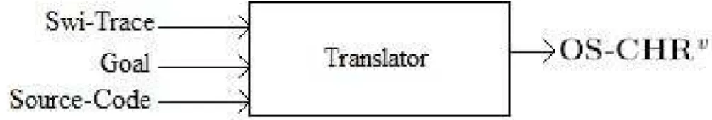
The Wake port is traced when a built-in is solved, in this case the constraint was reactivated because C7 = r.

6.3

Transforming SWI Tracer into OS-CHR

The SWI’s output is not enough to perform a translation to OS-CHR∨

. We do need information about what was the goal passed (to map all variables) and access to the source-code (get the rule names). The inputs and outputs of the algorithm is illustrated by figure4. The Translator’s algorithm will be explained by example.

Figure 4: Translator structure

For the Wake port the we have to look to previous values of the trace and determine what BIC solving fired this transition and also a Reactivate event will be produced. In this case C1 = a0 was the cause.

CHR: (3) Wake: node(r1,a0) # <359>

-> [61,Wake,[=,C1,a0],[woken,[[node,r1,C1,359]]],360] ++

[62,Reactivate,[node,r1,a0,359],@61,360] Some ports have direct connection with OS-CHR∨

: Call and Exit. All others ports will need a computation using the generated SWI trace. The Insert port is ignored because is redundant with the port Call.

CHR: (1) Call: edges # <330> ->

For the tryRule map, we have to look the source code and try to find what is the rule name for that transition, and while generating the trace we keep track of the active constraint. CHR: (7) Try: node(r4,a0) # <371>, edge(r4,r5) # <340>,

node(r5,a0) # <375> ==> a0=a0 | fail. ->

GT: [102,TryRule,failure@,[node,r5,a0,375],[keep,[[node,r4,a0,371], [edge,r4,r5,340], [node,r5,a0,375]]],[remove,[]],

[guard,[[=,a0,a0]]],376]

ApplyRule is the most complicated map, we have to link(@) with the tryRule and check if it has a disjunctive body, if it is we have keep track to link correctly with a possible failure status; it can generate a lot of trace event depending on how many constraints were added/removed and possibly a split transition. The link function will recover the real name of the variable, in this case _G9245 = C8

CHR: (9) Apply: node(r8,_G9245) # <390> ==> _G9245=a0; _G9245=a1;_G9245=a2;_G9245=a3. -> [141,ApplyRule,@140,[addrdc],[addbic,[=,C8,a0],[=,C8,a1], [=,C8,a2],[=,C8,a3]],[keep,[[node,r8,C8,390]]], [remove,[]],[match,[node(_,C)=node(r8,C8)]], [node,r8,C8,390],391] ++ GT: [142,Split, @141, 391]

The Exit port has a direct map with OS-CHR∨_.

CHR: (2) Exit: edge(r1,r9) # <332> ->

GT: [4,Drop,[edge,r1,r9,332],333]

The Fail port will produce a Fail event with its cause, a rule witch body contains the f alse built-in.

CHR: (6) Fail: node(r5,a0) # <375> ->

[109,Fail,@108,376]

6.4

Trace Querying

The produced generic trace is represented by a sequence of java objects. The language we choose for querying the trace is the SQL for Java Objects (JoSQL), its implementation can be found here8

.

These are some examples of query in JoSQL: (on a trace of example6)

• SELECT * FROM trace WHERE type =’ApplyRule’ AND (name=’wrong@’ OR name=’node1@’ OR name=’node2@’) Will select the trace of the execution of rules: wrong, node1,node2. • SELECT * FROM trace WHERE type =’Split’ OR type =’Fail’ Will select all split and

fail transition.

• SELECT addrdc,remove,addbic FROM trace WHERE type =’ApplyRule’

The last query is more general and can by used by any application which need to handle a current state of the constraint store.

6.5

Trace Analyzer

A Pretty Printer Analyzer was developed. This analyzer has a JoSQL query as parameter and prints the events that match the query. The OS-CHR∨

trace for leq with the goal leq(A,B),leq(B,C),leq(C,A) is depicted. All events and attributes were selected by JoSQL, they are listed in Section3.3.

[0,ActivateRDC,[leq,A,B,201],202] [1,Drop,[leq,A,B,201],202] [2,ActivateRDC,[leq,B,C,202],203] [3,TryRule,transitivity@,[leq,B,C,202],[keep,[[leq,A,B,201], [leq,B,C,202]]], [remove,[]],[guard,[]],203] [4,ApplyRule,@3,[addrdc,[leq,A,C]],[addbic],[keep,[[leq,A,B,201], [leq,B,C,202]]],[remove,[]],[match,[leq(X,Y)=leq(A,B)], [leq(Y,Z)=leq(B,C)]],[leq,B,C,202],203] [5,ActivateRDC,[leq,A,C,204],205] [6,Drop,[leq,A,C,204],205] [7,Drop,[leq,B,C,202],205] [8,ActivateRDC,[leq,C,A,205],206] [9,TryRule,antisymmetry@,[leq,C,A,205],[keep,[]], [remove,[[leq,C,A,205], [leq,A,C,204]]],[guard,[]],206] [10,ApplyRule,@9,[addrdc],[addbic,[=,C,A]],[keep,[]], [remove,[[leq,C,A,205], [leq,A,C,204]]], [match,[leq(X,Y)=leq(C,A)],[leq(Y,X)=leq(A,C)]],[leq,C,A,205],206] [11,Wake,[=,C,A],[woken,[leq,B,C,202],[leq,A,B,201]],206] [12,Reactivate,[leq,B,A,202],@11,206] [13,TryRule,antisymmetry@,[leq,B,A,202],[keep,[]], [remove,[[leq,B,A,202], [leq,A,B,201]]],[guard,[]],206] [14,ApplyRule,@13,[addrdc],[addbic,[=,B,A]],[keep,[]], [remove,[[leq,B,A,202], [leq,A,B,201]]], [match,[leq(X,Y)=leq(B,A)],[leq(Y,X)=leq(A,B)]],[leq,B,A,202],206] [15,Drop,[leq,A,A,202],206] [16,Drop,[leq,A,A,205],206]

7

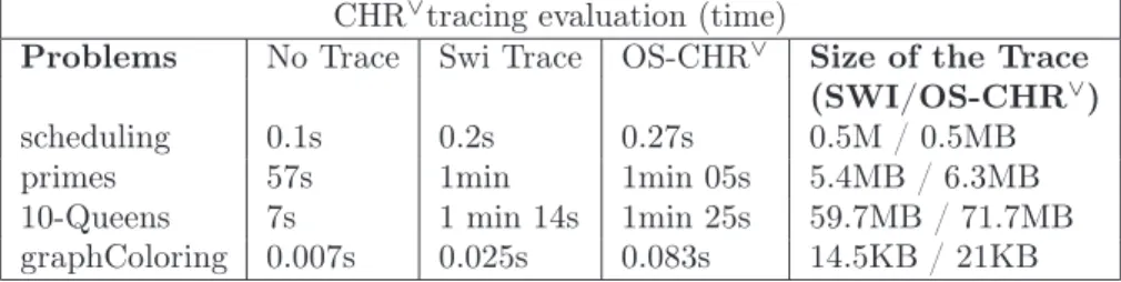
Experimentation

To evaluate our approach 3 benchmarks were set: 10-Queens, primes9 _{and a compiled example}

of scheduling from CHORD[4], available on its test folder, the reason for choosing a CHORD example was the complexity, more than 100 rules. All results are shown in the following table.

All the experiments were performed on a PC with Pentium Core 2 Duo processor running at 2,4 GHz, with 4 GB of RAM and 1.5GB were reserved to the Java heap. The Prolog trace generator and the trace querying process are two different process as described by Langevine[15]. The results are depicted in the table 4. Each line corresponds to a program. The firts column gives the execution time without tracing (trace off); the second, the execution time with

production of the SWI trace (trace on), the third the time in generic trace mode, and the last column gives the ratio between the sizes of both traces.

CHR∨

tracing evaluation (time) Problems No Trace Swi Trace OS-CHR∨

Size of the Trace (SWI/OS-CHR∨

) scheduling 0.1s 0.2s 0.27s 0.5M / 0.5MB primes 57s 1min 1min 05s 5.4MB / 6.3MB 10-Queens 7s 1 min 14s 1min 25s 59.7MB / 71.7MB graphColoring 0.007s 0.025s 0.083s 14.5KB / 21KB

Table 4: Experiments The following queries were done:

scheduling> g []. %starts chord computation

primes> candidates(8000). %calculates primes upto 8000

10-Queens> solveall(10,N,S). % give all solutions for 10 Queens.

graphColoring> edges, l([r1,r7,r4,r3,r2,r5,r6],[C1,C7,C4,C3,C2,C5,C6]). %graph with 7 edges

We observe that there is an (expected) slowdown in debugging modes (SWI trace and generic trace). It is slightly higher for the generic trace as it uses the SWI trace. Querying the generated trace does not slowdown more, since it can be done in paralel with trace generation.

For the selection of subtraces, tests executed on JoSQL show that that a list of 1,000,000 generic trace events can be queried in about 1.5s.

It must be noted that we limit the queries to patterns attached to a single event, limiting thus the complexity of the queries. Sophisticated queries envolving undetermined number of trace events could speed up seriously the performances.

8

Discussion

Several aspects of such a generic trace were explored on [17], in particular its relations with components software development, the use of the fluent calculus to prototype traces and the use of object oriented specification methods. The generic trace presented in that work is thus limited to the simple theoretical operational semantics ωt[10] and therefore is less precise than the one

given here.

Our approach of the observational semantics relies to abstract interpretation. The OS is similar to the “Observable Semantics” of Lucas [16] or the partial trace semantics of Cousot [3]. The parameters used to describe the execution states are, as expressed by Lucas, “syntactic objects used to represent the conduct of operational mechanisms”. The traces are abstract representations of CHR∨

semantics which allow to take into account the sole details we want to consider as common to different implementations. The (abstraction) relations between a generic trace and the traces of specific implementations of solvers are explored in [6], together with a compliance proof method. Furthermore the generic trace contains a set of details considered as useful in several debugging tasks with several levels of refinement or observation. It could be

enriched according to different needs10_{, or refined without changing the semantics of the already}

existing one.

This way to proceed is opposite to the frequently adopted approach as, in particular, in [18], where a set of (visual) debugging tools is defined together with their input data, which consists of a restricted trace containing the minimal needed information. In our approach, we specify a semantically rich trace which can be used as input data for a potentially larger set of tools. The choice of the data to trace is made on the basis of a high level operational semantics, not on the basis of some specific debugging need. However the generic trace is designed in such a way that most of debugging tools devoted to the analysis of CHR resolution behavior may find in this trace what they need. As a consequence, based on this observational semantics, the work of implementation of the tracer and the work of designing debugging tools can be performed independently.

One may however feel that implementing a full generic trace is too much work demanding or that the resulting tracer performance will be considerably slow down. It has been shown in [15] that a generic approach may have more advantages than drawbacks in the sense that there may be a good trade-off between a very detailed generic trace (based on a more refined operational semantics) and the use of a trace driver able to query efficiently the generic trace, with a significant improvement in portability of debugging tools. We have shown here, that the implementation of the CHR∨

generic trace in SWI-Prolog CHR implementation can easily be performed on the top of an existing tracer, resulting in a generic tracer practically as efficient as the original one on which it is based.

9

Conclusion

We have presented a first observational semantics of CHR∨

(a formal specification of a CHR∨

generic tracer), and two prototypes; the first is an executable operational semantics in Prolog which may produce a virtual generic trace; the second is a generic tracer of SWI CHR, based on the CHR SWI Prolog trace. The first helped to improve the quality of the formal operational semantics (in fact several corrections and/or improvements have been detected). The SWI CHR generic trace prototype shows that the generic trace can be easily and efficiently implemented on existing CHR∨

implementations. The interest of the “generic approach” leads in the portability of analysis tools developed on the basis of this trace and the variety of possible trace based applications.

We do not claim that the CHR∨

observational semantics which is presented here is the ultimate one. More refined observational semantics could be considered, including several levels of refinements (for example combining with Prolog semantics in Prolog based implementations); we just have shown that this approach can be realistic and useful in a great variety of CHR based software development.

Future work will concern more experimentation and improvements of the generic trace, OO based CHR implementation including a generic trace, and generic trace for hybrid constraint solvers.