Defining the human endothelial transcriptome
Texte intégral
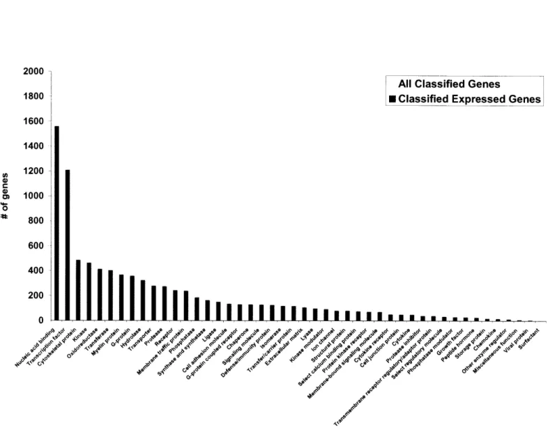
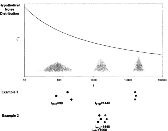
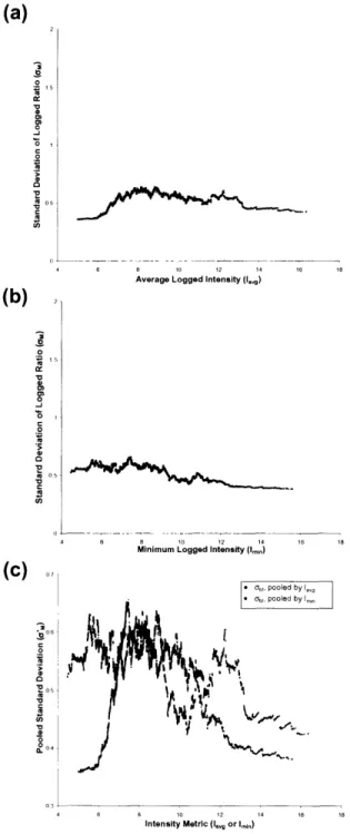
Figure


Documents relatifs
Sex workers (female , male or transvestite), journalists, police, small shopkeepers, street vendors and so on are very important. to prevent sexually transmitted diseases
Health workers must recognize that - although conflict is political - they, like other development workers, have a significant social role to play, and that direct
Wanneer het hout gekleurd moet worden gefixeerd, wordt aangeraden om aan alle kanten een eerste laag met een houtbeschermingsmiddel (bescherming tegen besmetting door schimmels
Using her mind power to zoom in, Maria saw that the object was actually a tennis shoe, and a little more zooming revealed that the shoe was well worn and the laces were tucked under
~ber 5 willkiirlichen Punkten des R.~ gibt es eine Gruppe yon 32 (involutorischen) Transformationen, welche auch in jeder anderen iiber irgend 6 besonderen
At that time the com pany, under the direction of Peter Z inovieff, was exploring the possibilities of using mini computers to control electronic music instruments.. My job was
Research Resource Identifiers (RRIDs) should reduce the prevalence of misidentified and contaminated cell lines in the literature by alerting researchers to cell lines that are on
Homework problems due December 10, 2014.. Please put your name and student number on each of the sheets you are
