HAL Id: hal-01134194
https://hal.archives-ouvertes.fr/hal-01134194
Submitted on 23 Mar 2015
HAL is a multi-disciplinary open access
archive for the deposit and dissemination of
sci-entific research documents, whether they are
pub-lished or not. The documents may come from
teaching and research institutions in France or
abroad, or from public or private research centers.
L’archive ouverte pluridisciplinaire HAL, est
destinée au dépôt et à la diffusion de documents
scientifiques de niveau recherche, publiés ou non,
émanant des établissements d’enseignement et de
recherche français ou étrangers, des laboratoires
publics ou privés.
Optimal Transport using Helmholtz-Hodge
Decomposition and First-Order Primal-Dual Algorithms
Morgane Henry, Emmanuel Maitre, Valérie Perrier
To cite this version:
Morgane Henry, Emmanuel Maitre, Valérie Perrier. Optimal Transport using Helmholtz-Hodge
De-composition and First-Order Primal-Dual Algorithms. 2015 IEEE International Conference on Image
Processing (ICIP), Sep 2015, Quebec City, QC, Canada. pp.4748-4752, �10.1109/ICIP.2015.7351708�.
�hal-01134194�
OPTIMAL TRANSPORT USING HELMHOLTZ-HODGE DECOMPOSITION AND
FIRST-ORDER PRIMAL-DUAL ALGORITHMS
Morgane Henry, Emmanuel Maitre and Val´erie Perrier
University of Grenoble-Alpes
Laboratoire Jean Kuntzmann
St Martin d’H`eres, France
ABSTRACT
This work deals with the resolution of the optimal trans-port problem between 2D images in the fluid mechanics framework of Benamou and Brenier formulation [1], which numerical resolution is still challenging even for medium-sized images. We develop a method using the Helmholtz-Hodge decomposition [2] in order to enforce the divergence-free constraint throughout the iterations. We then show how to use a first order primal-dual algorithm for convex problems of Chambolle and Pock [3] to solve the obtained problem, leading to a new algorithm easy to implement. Besides, nu-merical experiments demonstrate that this algorithm is faster than state of the art methods and efficient with real-sized images.
Index Terms— Convex optimization, optimal transport, proximal splitting, image processing, Helmholtz-Hodge de-composition
1. INTRODUCTION
Optimal transport is a domain with an increasing number of applications in economy [4], machine learning [5] or partial differential equations [6, 7]. The optimal transport problem defines a metric between densities [8], which appears to be relevant in image processing [9, 10]. The development of ef-ficient new algorithms for the calculus of the optimal trans-port between two densities is still a challenge, especially for real-sized images. In this paper we are interested in the Be-namou and Brenier formulation [1], who placed the problem in a context of fluid mechanics by adding a time dimension. They developed an algorithm based on the minimization of a functional which preserves the mass, using an augmented Lagrangian. Existing algorithms [10, 1], require a projection onto the divergence-free constraint at each iteration of the al-gorithm. This corresponds to solve a 3D Poisson equation at each time step for a 2D image. To reduce the computa-tional cost, we decided to work directly in the space of con-straints for the functional to minimize. Indeed, this will get This work is supported by the French Agence Nationale de la Recherche (ANR, Project TOMMI) under reference ANR-11-BS01-014-01.
rid of solving the Poisson equation, and speeding up the algo-rithm. The preservation of the constraint will be given by the Helmholtz-Hodge decomposition [2] of divergence-free ve-locities, applied to the vector formed by the time-dependent densities and momentum. This allows to rewrite the func-tional of Benamou-Bernier in terms of a stream function, and we show that the first order primal-dual algorithm for convex problems of Chambolle Pock [3] can be easily adapted for finding the minimum of the new functional. The Chambolle-Pock method is nowadays widely used [11, 12], leading to fast implementations, since it can be easily speed up on parallel architectures. Therefore our method leads to a fast algorithm, simple to implement on imaging problems.
In the following, we begin by introducing the optimal trans-port framework in the first section. Then, we develop the decomposition we use to stay in the set of constraints. Af-terward, we apply a primal-dual algorithm dedicated to our functional. We finish by numerical experiments, comparing our algorithm to state of the art on several test cases.
2. THEL2MONGE-KANTOROVICH PROBLEM
Let Ω = (0, 1)2 and (ρ0, ρ1) ∈ L2(Ω), be two positive,
bounded densities with�
Ωρ0 =
�
Ωρ1 = 1. Let | · | be the
Euclidean norm in R2, theL2-Wasserstein distance (see for
example [8]) between ρ0and ρ1is defined by
d2(ρ0, ρ1)2= inf M
�
|M (x) − x|2ρ0(x)dx,
where the infimum is taken among the maps M transferring ρ0to ρ1, which means that∀A ⊂ Ω,�x∈Aρ1=�M (x)∈Aρ0.
The Monge-Kantorovich problem (MKP) amounts to deter-mine an application M which realizes this infimum. Be-namou and Brenier [1] rephrased the problem in a con-tinuum mechanics framework. Let consider a time inter-val (0, 1), we set Q = (0, 1) × Ω and V (Q) = {f ∈ (L2(Q))1+2, div
t,xf = 0}. We consider the densities
ρ(t, x) ≥ 0 and vector fields v(t, x) ∈ R2 verifying the
continuity equation
fort ∈ (0, 1) and x ∈ Ω, equipped with the initial, final and boundary conditions
ρ(0, x) = ρ0(x), ρ(1, x) = ρ1(x), ∀x ∈ Ω, (2)
ρv(t, x) · νΩ= 0, ∀t ∈ (0, 1), x ∈ ∂Ω,
where νΩ is the outward normal ofΩ. As proven in [1] (see also [8]), the square of theL2-Wassertein distance between
ρ0and ρ1verifies d2(ρ0, ρ1)2= inf � 1 0 � Ω ρ(t, x)|v(t, x)|2dxdt,
where the infimum is taken among all ρ, v satisfying (1) and (2). To obtain a convex problem with linear constraints, Be-namou and Brenier introduced the momentumm = ρv and obtained the following formulation
min (ρ,m)∈C J(ρ, m) = min (ρ,m)∈C � 1 0 � Ω J(ρ(t, x), m(t, x))dxdt, where ∀(ρ, m) ∈ R × R2, J(ρ, m) = |m|2 2ρ , if ρ> 0, 0, if(ρ, m) = (0, 0), +∞, otherwise, (3) and the affine space of constraints reads
C := {(ρ, m), divt,x(ρ, m) = 0, m(·, x)·νΩ = 0, ∀ x ∈ ∂Ω,
ρ(0, ·) = ρ0, ρ(1, ·) = ρ1}.
We present below an algorithm working directly in the set of constraintsC.
3. REFORMULATION OF THE PROBLEM USING HELMHOLTZ-HODGE DECOMPOSITION To work in C, we use the orthogonal decomposition of L2(Q)1+2, detailed in [2]. The vector field v = (ρ, m) ∈
V (Q) has the following Helmholtz-Hodge decomposition: (ρ, m) = ∇ × φ + ∇h,
where we will denote∇ = ∇t,x, in the following. Moreover
φ∈ (H1
0(Q))3, andh ∈ H1(Q)/R and we have also divφ =
0. Because (ρ, m) is divergence-free we obtain � Δh = 0 in Q,
∂h
∂νQ = (ρ, m) · νQon ∂Q,
(4) where νQ is the outward normal of Q. So we have first to
solve the system (4) to obtainh, which is no more than a Pois-son equation with known boundary conditions. Then, know-ingh, we have to find the minimum of our new energy
J(∇ × φ) = � 1 0 � Ω F (∇ × φ(t, x) + ∇h(t, x))dxdt, (5) whereF : (X, Y ) �→|Y |2X2.
4. FIRST ORDER PRIMAL-DUAL ALGORITHM The method described by Chambolle and Pock in [3], allow-ing to minimize energies of the form (5), uses a primal-dual formulation (see [13]) of the form:
min
φ maxz �Kφ, z� + ιC0(φ) − J
∗(z). (6)
We considerK = ∇×, the curl operator, which is a linear continuous operator from(H1(Q))3to(L2(Q))3, the
Legen-dre transform of J (see [14]) J∗ : (L2(Q))3 → [0, +∞) and
ιC0 : (H
1(Q))3 → [0, +∞), the indicator function of the
setC0 := {(ρ, m), m(·, x) · νΩ = 0, ∀ x ∈ ∂Ω, ρ(0, ·) =
ρ0, ρ(1, ·) = ρ1}, which are proper, convex, lower
semicon-tinuous functions . It has been shown in [15] that for θ = 1 and στ||K||2 < 1, φk computed with the following
algo-rithm, converges to the solution of (6): Algorithm 1. Initialization: τ, σ > 0, θ ∈ [0, 1], (φ0, z0 = Kφ0, ˜φ0 = φ0). Iterations: zk+1= prox J∗(z k+ σ(K ˜φk)) φk+1= proxιC0(φ k− τ K∗zk+1) ˜ φk+1= φk+1+ θ(φk+1− φk).
Detailing the steps of the algorithm. The discrete objec-tive functional J reads for(ρ, m) defined on the centered grid Gc(defined in section 5):
J(ρ, m) = �
k∈Gc
J(ρk, mk), (7)
where the functionalJ is defined in (3), and then, proxγJ(x) = (proxγJ(xk))k∈Gc.
As proved in [1], the Legendre transform of J is the indicator function of a convex set, J∗= i
PJwhere � P J= {(z1, z2); ∀k ∈ Gc, (z1, z2)k∈ PJ} PJ = {(t, x) ∈ R × R2, t +|x| 2 2 ≤ 0}.
This implies thatproxγJ∗is the projection onto the paraboloid
PJ, which we will denote by PPJ. As we work on the
con-straint setC, (ρ, m) = ∇ × φ + ∇h, we now define a new functional, for(a, b) = ∇ × φ:
Jh(a, b) = J(a + ∂th, b + ∇xh) = � k∈Gc Jh(a, b) = � k∈Gc J(a + ∂th, b + ∇xh). (8)
This enables us to deduce fromJ∗ the form ofJ∗ h and the
form ofproxγJ∗
h from the one ofproxγJ∗. If we denotec =
Proposition 1. One has for allc ∈ R1+n J∗ h(c) = J∗(c) − �∇h, c�, and proxγJ∗ h(c) = proxγJ∗(c − γ∇h).
Finally, the primal-dual algorithm reads in our case Algorithm 2. Initialization: τ, σ > 0, θ ∈ [0, 1], (φ0, z0 = Kφ0, ˜φ0 = φ0). Iterations: zk+1= P PJ(z k+ σ(∇ × ˜φk+ ∇h)) φk+1= PC0(φ k− τ ∇∗× zk+1) ˜ φk+1= φk+1+ θ(φk+1− φk).
The computation of PPJ amounts to solve a third order
equation by grid point, while PC0 merely corresponds to set
the boundary conditions to zero.
5. NUMERICAL APPLICATION TO IMAGE TRANSPORT
5.1. Discrete setting
We now describe the discrete grids used in the computations. Centered grid. The regular grid
Gc= {ti, xj, yk}1≤i≤M, 1≤j≤N, 1≤k≤P,
withti = Mi , xj= Nj, yk = Pk the discrete locations in the
domainQ, is used to evaluate ρ and m.
Staggered grid. We introduce two staggered grids to evaluate the divergence and the curl operators. The gridGs1provides
a discretization coherent with the divergence of(ρ, m) and is defined by:
Gs1t = {ti−1/2, xj, yk}1≤i≤M +1, 1≤j≤N, 1≤k≤P,
Gs1x = {ti, xj−1/2, yk}1≤i≤M, 1≤j≤N +1, 1≤k≤P,
Gs1y = {ti, xj, yk−1/2}1≤i≤M, 1≤j≤N, 1≤k≤P +1.
Our staggered gridGs2for φ such that∇ × φ is on the
stag-gered gridGs1:
Gs2t = {ti, xj−1/2, yk−1/2}1≤i≤M, 1≤j≤N +1, 1≤k≤P +1,
Gs2x = {ti−1/2, xj, yk−1/2}1≤i≤M +1, 1≤j≤N, 1≤k≤P +1,
Gs2y = {ti−1/2, xj−1/2, yk}1≤i≤M +1, 1≤j≤N +1, 1≤k≤P.
Interpolation operator. To go to the centered grid from the gridGs1we need an interpolation operator, which is:
ρ, m (Gs1) → ρ, m (Gc)
ρi−1/2,j,k ρi,j,k= (ρi+1/2,j,k+ ρi−1/2,j,k)/2
mi,j−1/2,k → m1i,j,k= (m1i,j+1/2,k+ m1i,j−1/2,k)/2
mi,j,k−1/2 m2i,j,k= (m2i,j,k+1/2+ m2i,j,k−1/2)/2
and its adjoint operator to go fromGctoGs1.
Curl, gradient and divergence operators. The discrete gra-dient is a vector of matrices∇v = (∇tv ∇x1v ∇x2v) . We
use finite differences to compute the gradient, which has, for first component
∇tvi,j,k= vi+1/2,j,k− vi−1/2,j,k, ifi ≤ M,
and the adjoint divergence operator
∇t.vi−1/2,j,k= −v1,j,k ifi = 1 vi,j,k− vi−1,j,k if2 ≤ i ≤ M vM,j,k ifi = M + 1.
The curl operator we use is derived from the gradient operator. In order to use the primal dual algorithm we need to define the discrete adjoint operator of the curl. Because the curl operator is given by the following matrix
0 −∇x2 ∇x1 ∇x2 0 −∇t −∇x1 ∇t 0
the appropriate adjoint curl operator has to be the opposite of the curl derived from the divergence operator.
5.2. Numerical applications
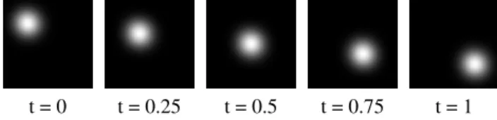
For the performance evaluation we compare our algorithm (PDHH) to the primal-dual algorithm developed in [10] that we will denote PDPOP in the following. We computed it = 106iterations in the case of the transport of two isotropic
Gaussians with the same variance, and we plot the estimated density in Figure 1: the solution is displayed in black and grey, black being 0 and white being 1, and will be denoted (ρs, ms). We use a grid of N × P = 64 × 64 discretization
points for ρ0and ρ1 andM = 64 points for the time t. In
the following we will use the parameters||K||2= 8, σ = 90,
τ = 0.99/Lσ and θ = 1. We choosed σ such that the errors onm and ρ are minimal after it = 50 iterations.
t = 0 t = 0.25 t = 0.5 t = 0.75 t = 1 Fig. 1. Display of the density ρ(t) obtained after it = 106
iterations.
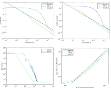
Figure 2 displays theL2error between ρ and ρ
sand between
m and ms, the functional J and the complexity, for 5000
iter-ations, for both algorithms PDPOP and PDHH in the example of Figure 1. It shows that despite our algorithm has not the best convergence rate during the first iterations, it converges quickly until we obtain theO(1/i) convergence rate. Indeed,
Fig. 2. Comparison at each iteration of theL2error between ρ
and ρsand betweenm and ms, the functional J and the
com-plexity, for 5000 iterations, for PDPOP algorithm and PDHH algorithm in the case of figure 1.
the decreasing of the functional in the constraint set has not the same behavior as in the PDPOP algorithm, where one has to project onto the divergence-free constraint space. Figure 2 also displays the computation time with respect to the num-berM = N = P of discretization points in one direction. It shows that the complexity of the two algorithms is linear of orderO(M3). But it depends also on the number of
itera-tions. The bigger the grid is, the better our algorithm behaves in comparison with the PDPOP algorithm. Moreover, this behavior increases with the number of iterations we run, as shown in Table 1.
The explanation is that we don’t have to solve a Poisson it = 100 it = 500 it = 1000 it = 5000 N = 16 1.26 1.24 1.20 1.26 N = 32 1.28 1.41 1.45 1.31 N = 64 1.15 1.31 1.37 1.40 N = 128 1.32 1.21 1.42 1.46
Table 1. Ratios between cpu time per iteration for PDPOP algorithm and PDHH algorithm, for different numbers of it-erations and different sizes.
equation at each iteration. But contrarily to PDPOP, we have to evaluate a curl operator inK, which is slightly time-consuming.
Test on non convex densities. The next example of transport considers the case of irregular, non convex and non connected densities with compact support. Figure 3 shows the ability of our method to estimate the density ρ(t) for such initial and final densities.
t = 0 t = 0.25 t = 0.5 t = 0.75 t = 1 Fig. 3. Display of the density ρ(t) obtained after it = 106
iterations of a non-convex, non connected density with com-pact support on a gridM × N × P = 64 × 64 × 64.
Test on real images. As last example we compute the density ρ(t) for images representing clouds in different po-sitions. The results presented in Figure 4 are obtained for images discretized on a gridM = 30 for the time dimension andN × P = 100 × 68 for the space dimension.
t = 0 t = 0.25 t = 0.5 t = 0.75 t = 1 Fig. 4. Display of the density ρ(t) of an image of clouds. The first line represents ρ(t) obtained after it = 1.106 itera-tions of PDHH algorithm while the second line represents the L2interpolation.
6. CONCLUSION
We introduced a new algorithm for the optimal transport prob-lem between 2D images, which respects the divergence-free constraint throughout the iterations, and therefore gets rid of solving a 3D Poisson equation at each iteration. Besides, this algorithm is easy to implement, faster than state of the art methods, and efficient for real-sized images. Further im-provements of the method will include other divergence-free decomposition, and other formulations of the primdual al-gorithm.
7. REFERENCES
[1] J-D. Benamou and Y. Brenier, “A computational fluid mechanics solution to the monge-kantorovich mass transfer problem,” Numerische Mathematik, vol. 84, no. 3, pp. 375–393, 2000.
[2] V. Girault and P-A. Raviart, “Finite element methods for navier-stokes equations: theory and algorithms,” NASA STI/Recon Technical Report A, vol. 87, pp. 52227, 1986. [3] A. Chambolle and T. Pock, “A first-order primdual al-gorithm for convex problems with applications to
imag-ing,” Journal of Mathematical Imaging and Vision, vol. 40, no. 1, pp. 120–145, 2011.
[4] P-A. Chiappori, R. J. McCann, and L. P. Nesheim, “Hedonic price equilibria, stable matching, and optimal transport: equivalence, topology, and uniqueness,” Eco-nomic Theory, vol. 42, no. 2, pp. 317–354, 2010. [5] Y. Rubner, C. Tomasi, and L. J. Guibas, “A metric for
distributions with applications to image databases,” pp. 59–66, 1998.
[6] J. S. Moll J. A. Carrillo, “Numerical simulation of diffu-sive and aggregation phenomena in nonlinear continuity equations by evolving diffeomorphismss,” SIAM J. Sci. Comput., vol. 31, pp. 4305–4329, 2009.
[7] R. Jordan, D. Kinderlehrer, and F. Otto, “The variational formulation of the fokker–planck equation,” SIAM jour-nal on mathematical ajour-nalysis, vol. 29, no. 1, pp. 1–17, 1998.
[8] Villani C., Topics in optimal transportation, Number 58. American Mathematical Soc., 2003.
[9] J. Rabin, S. Ferradans, and N. Papadakis, “Adaptive color transfer with relaxed optimal transport,” pp. 4852– 4856, 2014.
[10] N. Papadakis, G. Peyr´e, and E. Oudet, “Optimal trans-port with proximal splitting,” SIAM Journal on Imaging Sciences, vol. 7, no. 1, pp. 212–238, 2014.
[11] J. C. Pesquet P. L. Combettes, L. Condat and B. C. Vu, “A forward-backward view of some primal-dual opti-mization methods in image recovery,” pp. 4141–4145, 2014.
[12] B. He and X. Yuan, “Convergence analysis of primal-dual algorithms for a saddle-point problem: From con-traction perspective,” SIAM Journal on Imaging Sci-ences, vol. 5, no. 1, pp. 119–149, 2012.
[13] R T. Rockafellar, Convex analysis, vol. 28, Princeton university press, 1997.
[14] H. H. Bauschke and P. L. Combettes, Convex anal-ysis and monotone operator theory in Hilbert spaces, Springer, 2011.
[15] A. Chambolle, “An algorithm for total variation min-imization and applications,” Journal of Mathematical imaging and vision, vol. 20, no. 1-2, pp. 89–97, 2004. [16] K. J. Arrow, L. Hurwicz, H. Uzawa, and H. B. Chenery,
Studies in linear and non-linear programming, vol. 2, Stanford University Press Stanford, 1958.
[17] P. L. Combettes and V. R. Wajs, “Signal recovery by proximal forward-backward splitting,” Multiscale Mod-eling & Simulation, vol. 4, no. 4, pp. 1168–1200, 2005.
[18] R. Yildizoglu, J-F. Aujol, and N. Papadakis, “Active contours without level sets,” pp. 2549–2552, 2012. [19] P. L. Combettes and J-C. Pesquet, “Proximal splitting
methods in signal processing,” in Fixed-point algo-rithms for inverse problems in science and engineering, pp. 185–212. Springer, 2011.
[20] J-J. Moreau, “Proximit´e et dualit´e dans un espace hilber-tien,” Bulletin de la Soci´et´e math´ematique de France, vol. 93, pp. 273–299, 1965.