HAL Id: hal-00298338
https://hal.archives-ouvertes.fr/hal-00298338
Submitted on 8 Jun 2007
HAL is a multi-disciplinary open access
archive for the deposit and dissemination of
sci-entific research documents, whether they are
pub-lished or not. The documents may come from
teaching and research institutions in France or
abroad, or from public or private research centers.
L’archive ouverte pluridisciplinaire HAL, est
destinée au dépôt et à la diffusion de documents
scientifiques de niveau recherche, publiés ou non,
émanant des établissements d’enseignement et de
recherche français ou étrangers, des laboratoires
publics ou privés.
data into large-scale sea ice models
V. Dulière, T. Fichefet
To cite this version:
V. Dulière, T. Fichefet. On the assimilation of ice velocity and concentration data into large-scale sea
ice models. Ocean Science, European Geosciences Union, 2007, 3 (2), pp.321-335. �hal-00298338�
www.ocean-sci.net/3/321/2007/
© Author(s) 2007. This work is licensed under a Creative Commons License.
Ocean Science
On the assimilation of ice velocity and concentration data into
large-scale sea ice models
V. Duli`ere and T. Fichefet
Universit´e Catholique de Louvain, Institut d’Astronomie et de G´eophysique Georges Lemaˆıtre, Louvain-la-Neuve, Belgium Received: 13 February 2007 – Published in Ocean Sci. Discuss.: 2 March 2007
Revised: 16 May 2007 – Accepted: 21 May 2007 – Published: 8 June 2007
Abstract. Data assimilation into sea ice models designed for
climate studies has started about 15 years ago. In most of the studies conducted so far, it is assumed that the improve-ment brought by the assimilation is straightforward. How-ever, some studies suggest this might not be true. In order to elucidate this question and to find an appropriate way to further assimilate sea ice concentration and velocity obser-vations into a global sea ice-ocean model, we analyze here results from a number of twin experiments (i.e. experiments in which the assimilated data are model outputs) carried out with a simplified model of the Arctic sea ice pack. Our ob-jective is to determine to what degree the assimilation of ice velocity and/or concentration data improves the global per-formance of the model and, more specifically, reduces the error in the computed ice thickness. A simple optimal inter-polation scheme is used, and outputs from a control run and from perturbed experiments without and with data assimila-tion are thoroughly compared. Our results indicate that, un-der certain conditions depending on the assimilation weights and the type of model error, the assimilation of ice velocity data enhances the model performance. The assimilation of ice concentration data can also help in improving the model behavior, but it has to be handled with care because of the strong connection between ice concentration and ice thick-ness. This study is first step towards real data assimilation into NEMO-LIM, a global sea ice-ocean model.
1 Introduction
In polar regions, the interactions between atmosphere and ocean are significantly modified by the presence of sea ice. Because of its high albedo and insulating behavior, sea ice largely affects the surface radiative balance and the oceanic
Correspondence to: V. Duli`ere
heat budget. In addition, the melting of weakly saline ice or the brine rejection occurring during ice formation induces variations in the sea surface salinity that affect the mixed layer dynamics and the ocean circulation. On the other hand, the ice dynamics plays an important part in modulating the momentum transfer from the atmosphere to the ocean.
During the past 35 years, the Arctic sea ice concentra-tion and moconcentra-tion have been widely observed with the aid of passive microwave sensors aboard satellites (e.g. Bjørgo et al., 1997; Cavalieri et al., 1997; Emery et al., 1997; Parkin-son et al., 1999; Comiso and Steffen, 2001; Cavalieri et al., 2003). Analysis of these records indicate that the Arctic sea ice extent has shrunk at an annual mean rate of about 0.30×10⁶km2 with strong interannual variability since the early 1970s (Cavalieri et al., 2003). Comparatively, the Arc-tic sea ice thickness is much less known.
Our knowledge of sea ice thickness in the Northern Hemi-sphere comes mainly from upward sonar profiling by sub-marines. Rothrock et al. (1999) compared ice draft data ac-quired by the Scientific Ice Expeditions (SCICEX) program in 1993, 1996 and 1997 with data from six cruises during the period 1958–1976. They found a decrease in the mean ice draft at the end of the melt season of about 1.3 m (i.e. 40%) in most of the deep-water areas of the Arctic Ocean. Comparing data from single cruises in 1996 and 1976 from Fram Strait to the North Pole, Wadhams and Davis (2000) reported a strik-ingly similar reduction in ice draft. In contrast, ice draft data collected during six submarine cruises from Alaska to the North Pole in 1991–1997 exhibit almost no change (Win-sor, 2001). From nine cruises from 1976 through 1994 on the Alaska-to-North Pole section, Tucker et al. (2001) found an abrupt thinning between the mid-1980s and early 1990s. No similar trend was however observed near the North Pole. Recently, a detailed analysis of submarine and modeled ice thicknesses (Holloway and Sou, 2002) has demonstrated that ice motion and high interannual variability make inference of trends from sonar transect data ambiguous, suggesting that
the available sonar data are insufficient to resolve the vari-ability of the Arctic ice thickness. Later, the thinning of the Arctic ice cover has been reconfirmed. Comparing 8 cruises spanning the years 1987–1997 in the Arctic Ocean, Rothrock et al. (2003) found a decrease in draft data of about 1 m over the 11-year span. Several other studies point towards a thin-ning of the Arctic ice cover (i.e. Yu et al. (2003); Perovich et al. (2003); Rigor and Wallace (2004); Fowler et al. (2004); Comiso (2002)). New techniques to measure the sea ice thickness from space are now being developed (e.g. Laxon et al., 2003; Yu and Lindsay, 2003; Kwok et al., 2004). Nev-ertheless, an accurate knowledge of past ice thickness vari-ations remains necessary in order to assess human-induced climate changes in the Arctic.
A number of regional or global ice-ocean general circu-lation models driven by atmospheric reanalysis data fields have been used to document the variability of the Arctic sea ice over the last few decades (e.g., Maslowski et al., 2000; Holloway and Sou, 2002; Fichefet et al., 2003; K¨oberle and Gerdes, 2003; Rothrock and Zhang, 2005; Timmermann et al., 2005). These models provide very useful information regarding the behavior of the ice pack. However, their abil-ity to simulate the shorter-term variabilabil-ity as well as sum-mer features of the ice cover remains rather limited. Con-sequently, hindcast simulations of Arctic sea ice often de-viate from reality. One way of estimating this might be to assimilate the available ice concentration and/or velocity ob-servations into the models. Assimilating data into numer-ical models has proven very useful in the atmospheric and oceanic modeling communities for many years (e.g. Ghil and Malanotte-Rizzoli, 1991). It is however a less common prac-tice in large-scale sea ice modeling.
Thomas and Rothrock (1989, 1993) have applied Kalman smoothing to passive microwave ice concentration data. They utilized a simple sea ice model, driven by velocities optimally interpolated from buoy motions, to form indepen-dent model-derived concentration estimates that were opti-mally blended with the concentration data. They then ana-lyzed seven years of first-year and multiyear ice concentra-tion data for the Arctic Ocean, which they divided into seven regions. Later, Thomas et al. (1996) extended this work to the calculation of ice thickness. They used observed ice mo-tions, winds and ice concentrations plus a thermodynamic sea ice model to produce spatially and temporally varying ice thickness distribution in the Arctic. By comparing their results with submarine ice thickness data, they found that, for the whole Arctic Ocean, their estimates agree with the observational data but show less spatial and temporal vari-ability. More recently, Lisaeter et al. (2003) demonstrated the assimilation of passive microwave ice concentration data into a comprehensive ice-ocean general circulation model of the Arctic Ocean using an ensemble Kalman filter. They con-cluded that the assimilation of ice concentration data is a vi-able way of controlling the simulated ice cover, but does not correct the generally underestimated model ice thickness.
The study of Meier et al. (2000) was the first attempt to assimilate observed ice motion data into a large-scale model of the Arctic sea ice cover in order to maximize the model accuracy. These authors employed an optimal interpolation scheme to assimilate ice velocity data derived from passive microwave imagery. They found that the assimilation sub-stantially reduces the error standard deviation and improves the correlation of the simulated motions relative to buoy ob-servations. Nevertheless, they noticed that the assimilation induces unrealistic changes in ice thickness near the Green-land coast and the Canadian Archipelago as well as in the outflow of ice mass through Fram Strait. In other studies, Meier and Maslanik (2001a,b) demonstrated the utility of a data assimilation approach for improving the model es-timation of buoy trajectories and for investigating synoptic events in the Arctic sea ice drift. Later, Arbetter et al. (2002) combined satellite-derived and modeled ice velocities in a large-scale Arctic sea ice model to simulate the anomalous summer ice retreats observed in 1990 and 1998. For both years, the computed ice extent appears in better agreement with observational estimates when ice velocity data are as-similated, but excessive ice melt occurs in the central pack. Meier and Maslanik (2003) further investigated the effects of local conditions (namely, the proximity to the coast, the ice thickness and the wind forcing) on Arctic remotely sensed, modeled and assimilated ice velocities. They showed that the optimal interpolation assimilation technique improves the quality of the ice motion throughout most ranges of wind speed and ice thickness both in coastal and non-coastal re-gions. Their results also suggest that the use of assimilation weights optimized for representative environmental condi-tions would further reduce errors and yield greater benefits from assimilation. Very recently, Dai et al. (2006) showed that efforts to adjust a sea ice model by altering the frictional loss parameter have limited effects in the cases where ob-served ice motions are assimilated because the assimilation essentially bypasses the model dynamics. In parallel, Zhang et al. (2003) conducted a hindcast simulation of the Arctic sea ice variations over the period 1992–1997 with a regional ice-ocean general circulation model in which buoy and pas-sive microwave ice motion data were assimilated by means of an optimal interpolation scheme. Assimilation was found to significantly improve the modeled ice motion, with substan-tially reduced stoppage, which in turn leads to strengthened ice outflow at Fram Strait, enhanced ice deformation and ice drafts that are slightly closer to those derived from submarine measurements. Lindsay et al. (2003) extended this work for a 10-month period in 1997 and 1998. Comparisons of ice ve-locity Radarsat Geophysical Processor System (RGPS) mea-surements to the modeled velocities showed excellent agree-ment from the model-with-data-assimilation run but poorer agreement for the model-only run. However, the deforma-tion from the data assimiladeforma-tion run was in modest agreement with observations, suggesting that some model aspects need improvement.
Very recently, Lindsay and Zhang (2006) extended the work of Zhang et al. (2003) by incorporating in their model of the Arctic ice-ocean system a nudging scheme with a non-linear weighting function to assimilate passive microwave ice concentration data. They observed that the assimilation of ice concentration alone increases the ice draft bias, espe-cially in the marginal seas, but improves the correlation with ice draft measurements made by upward looking sonars on submarines and moorings. When both ice concentration and velocity data are assimilated, an improvement in the ice draft comparison is obtained, but a significant bias still exists in the large-scale ice thickness pattern. It should be noted that Lindsay and Zhang (2005) used this experimental set-up to investigate the causes of the recent changes of the Arctic ice pack.
The studies mentioned above indicate that data assimila-tion generally improves the model estimate of the assimi-lated variable(s) but can deteriorate the simulation of other variables. So far, no detailed assessment of the impact of data assimilation on the global performance of a large-scale sea ice model has been performed. This is mainly due to our very limited knowledge of both modeling and observa-tional errors (Weaver et al., 2000). In order to circumvent this difficulty, we analyze here results from a number of twin experiments (i.e. experiments in which the assimilated data are model outputs) carried out with a simplified model of the Arctic sea ice pack. This method to approach data assimi-lation into sea ice models is an interesting first step towards real data assimilation into NEMOLIM (Timmermann et al., 2005), a global sea ice-ocean model. Our aim is to deter-mine to what degree the assimilation of ice velocity and/or concentration data improves the overall performance of the model and, more specifically, reduces the error in the com-puted ice thickness.
The rest of the paper is organized as follows. Section 2 provides a brief description of the model and forcing. The assimilation scheme and experimental design are presented in Sect. 3. Section 4 is devoted to the discussion of the re-sults. A summary and some concluding remarks are finally given in Sect. 5.
2 Model formulation and forcing
The model used in this work is a simplified two-level, thermodynamic-dynamic sea ice model. This model takes into account the most relevant sea ice processes while being inexpensive in CPU time. As mentioned above, this model is used to have a first-guess estimate on data assimilation into a sea ice model. Therefore, it is not meant to reproduce exactly the sea ice features and should be taken as a “toy-model”.
The main model variables are the ice thickness, hi, the ice
concentration, Ai, and the ice velocity, ui. The presence of
snow on top of sea ice is neglected. However, a prescribed, monthly varying surface albedo that takes into account the
presence of snow is used (Semtner, 1976). Local changes in ice thickness and concentration are calculated from the following conservation laws:
∂Aihi
∂t = −∇ ×(uiAihi) + Sh (1)
∂Ai
∂t = −∇ ×(uiAi) + SA (2)
where t is the time and Sh and SA are thermodynamic sink
or source terms computed as in Hibler (1979). The vertical growth/decay rate of the ice is determined by the zero-layer model proposed by Semtner (1976). When ice is present in a grid cell and the heat budget of the open-water area becomes negative, ice of thickness ho=0.5 m (Hibler, 1979) is
accu-mulated onto the side of the existing ice. The thickness of the newly formed ice is then averaged with that of the older ice to obtain a single value. Furthermore, a minimum open-water fraction of 0.5% is prescribed to simulate the fact that cracks or leads are always present inside the pack owing to unresolved dynamical effects. Ice dynamics is computed by assuming that sea ice behaves as a two-dimensional contin-uum in dynamical interaction with atmosphere and ocean. A first estimate of the sea ice velocity is obtained from the so-called free-drift equation:
−mf k × ui + τa+ τw=0 (3)
where m is the ice mass per unit area, f is the Coriolis param-eter, k is a vertical unit vector and τaand τw are the forces
(per unit area) due to air and water drags, respectively. Note that the force (per unit area) associated with the tilt of the sea surface is neglected. The computed velocity is then corrected to avoid excessive ice build-up in regions of convergent ice motion due to the neglect of internal ice forces. Following Kreyscher et al. (2000), the ice velocity is set equal to zero where (1) the ice thickness exceeds 3 m and (2) the ice would be transported into an area with thicker ice. Applied as it is, this correction causes a velocity gradient that is too steep and causes problems when assimilating data into the model. To prevent those troubles, it is necessary to smooth the transi-tion by applying a hyperbolic tangent reductransi-tion factor to the ice velocity as a function of hi.
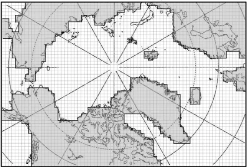
An upstream scheme with anti-diffusion is used for ad-vection (Smolarkiewicz, 1983). First the thermodynamical equations then the dynamical ones are solved on a Cartesian grid covering the Arctic Ocean and adjacent seas, with a spa-tial resolution of about 100 km (Fig. 1). A time step of one day is employed.
Daily 2 m air temperatures and 10 m winds from the Na-tional Centers for Environmental Prediction/NaNa-tional Cen-ter for Atmospheric Research (NCEP/NCAR) (Kalnay et al., 1996) are utilized to drive the model. The other atmospheric input fields consist of climatological monthly surface rela-tive humidities (Trenberth et al., 1989) and cloud fractions (Parkinson and Washington, 1979). The surface fluxes of
Fig. 1. Model domain and grid.
Fig. 2. Schematic representation of the experimental design.
heat are determined from these data using empirical param-eterizations described by Goosse (1997). The oceanic heat flux at the base of the ice layer, Fb, is given by:
Fb=ρwcpwhmlγt(Tobs−Tml) (4)
where ρwis the density of seawater, cpwis the specific heat
of seawater, hmlis the mixed-layer depth (30 m), γt is a time
constant (6×10⁻⁸s−1), Tml is the model mixed-layer
tem-perature and Tobsis the monthly mean observed mixed-layer temperature given by the Polar Science Center Hydrographic Climatology (PHC, Steele et al., 2001). When sea ice is present in a grid cell, Tml is set equal to the freezing point
of seawater (271.2 K according to Semtner, 1976). Ice is not allowed in grid cells where Tml is greater than the freezing
point of sea water. In ice-free grid cells, Tml is determined
from the heat budget of the mixed layer. It is worth men-tioning that Fb is included in this heat budget to implicitly
account for the advection of heat by oceanic currents. If Tml
reaches the freezing point, then a new ice layer of thickness
hoforms at the ocean surface. The momentum fluxes at the
various interfaces are obtained from standard bulk formulas described by Goosse (1997). For the quadratic drag coeffi-cients between air and ice and between ice and water, we use constant values of 1.2×10⁻³ (McPhee, 1980) and 5×10⁻³ (Timmermann et al., 2005), respectively. The ocean is as-sumed to be motionless.
Results of data assimilation are assumed to be somewhat model dependent. Hence, it would be appropriate to intro-duce physical processes, like among other things, deforma-tion from shear, brine pocket release or ocean feedbacks in the model. However, for a more complete understanding of model results, for CPU time reasons and because we plan to later test data assimilation with NEMOLIM (a more compre-hensive global ice-ocean model), we decided to run experi-ments with the model described above.
3 Experimental design and assimilation scheme
3.1 Experimental design
As mentioned in Sect. 1, the major problem when assimi-lating data into large-scale sea ice models comes from our rather poor knowledge of both model and observation errors. To overcome this problem, we build an idealized “observa-tional” dataset with the model and perform so-called twin experiments (Fig. 2).
A control run from 1977 to 2000 is first conducted. The model is initialized with a 3 m-thick and 99.5%-compact ice cover over the entire domain. Outputs for years 1995 and 1996 are regarded as the “reality” or true state (hereafter
Table 1. Acronyms of the twin experiments performed with the model. XX and YY represent the values of the weights for ice velocity and concentration assimilation, respectively.
Thermodynamical Dynamical model model perturbation perturbation
Without data assimilation WA T WA D
Concentration data assimilation CA T XX CA D XX
Velocity data assimilation VA T YY VA D YY
Velocity and concentration data assimilation VCA T YY XX VCA D YY XX
referred to as TS) for those years (i.e. as observations without any error). Then, to account for model errors in estimating the TS, the model is perturbed and new experiments are car-ried out over the years 1995 and 1996. In order to introduce errors that remain consistent with the model physics, pertur-bations are applied to the model forcing. Two types of dis-turbance are considered. First, we use the surface air temper-atures of years 1992 and 1993 instead of those of years 1995 and 1996. In this case, the dynamic component of the model is regarded as perfect and the thermodynamic component as a source of errors. Second, the surface winds employed to compute the air-ice stress are replaced by those of years 1992 and 1993. This time, it is the thermodynamic component of the model which is considered as perfect and the dynamic component as a source of errors. The chosen perturbations are fairly strong. However, we also forced the model with weighted mixes of forcings from two different years. We ran several tests combining different years (not only 1992–1993 and 1995–1996). We also tested several weights. Neverthe-less, all experiments pointed towards the same conclusions. In this paper, we focused on the 1995–1996 period because it gives a good summary of all the experiments we have run. For the thermodynamic and dynamic perturbations, we as-sess how the assimilation of ice velocities and/or concen-trations from the TS improves the model behavior. Table 1 summarizes the various types of experiments made with the model.
The observation data sets are compiled from control ex-periment outputs. No noise is added. The impact of the data set quality on the assimilated results is not studied here, al-though it would be an interesting work to carry out.
Twin experiments are common practice in atmospheric and oceanic modeling (e.g. Lin et al., 2001; Fox et al., 2000). However, to our knowledge, it is the first time that simula-tions of this kind are performed with a sea ice model. Usu-ally, twin experiments are carried out in a forecasting per-spective, and thus the model is perturbed by changing initial conditions. Here, as the purpose is rather oriented toward re-analysis, we find more appropriate to alter the thermal and dynamical forcings.
3.2 Assimilation scheme
At each time step, an optimal interpolation scheme is used to assimilate ice concentration and ice velocity data into the model according to:
Aass=A + kA(Aobs−A) (5)
uass= u +ku(uobs− u) (6)
where the subscripts “ass” and “obs” stand for assimilated and observed data. While the ice velocity is updated at the end of the model velocity computation (before ice transport), the ice concentration update is done at the end of the model iteration. kA and ku are the weights for ice concentration
and ice velocity data assimilation, respectively, and are usu-ally determined through a least squares minimization of the error variance of the assimilated value compared to a statisti-cal true value (Meier et al., 2000; Lindsay and Zhang, 2006). However, the present experimental design provides one ob-servation per model grid cell with zero error. The weight should then be set to one, and observed data would directly be inserted into the model. Nevertheless, as shown in Sect. 4, a weight equal to 1 does not systematically give the best re-sults.
The assimilation technique used in this paper is simple but accurate enough for the purpose of our study. In particular, as shown in Sect. 4, it allows to underline a number of problems posed by the assimilation of ice concentration and/or velocity data into large-scale sea ice models.
4 Results
4.1 Control run
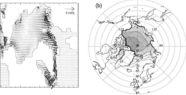
The model ice circulation averaged over 1979–1999 (Fig. 3a) exhibits many of the recurrent or permanent features of the observed ice motion (e.g. Emery et al., 1997). In particu-lar, the clockwise Beaufort Gyre, the Transpolar Drift Stream and the East Greenland Drift Stream are all reproduced. Note that the model has no river runoff and a motionless ocean. The magnitude of the ice velocity appears globally under-estimated. On average, the simulated ice drift tends to thin the ice off the Alaskan and Siberian coasts while increasing
Fig. 3. Annual mean ice velocities (a) and March ice thicknesses (b) from the control run averaged over the period 1979–1999. Scale vector for ice velocity is 3 cm s−1. Selected contours for ice thickness are 0.5, 1, 1.5, 2, 2.5 and 3 m.
the ice thickness by convergence and concomitant ridging off the Canadian Archipelago and the north coast of Greenland (Fig. 3b). The shape and magnitude of the simulated ice thickness contours are in general agreement with those de-rived from submarine sonar measurements (e.g. Bourke and Garrett, 1987). The most significant departure from current estimates is observed along the Canadian Archipelago and the north coast of Greenland, where the model generates too thin of an ice cover. This feature together with the gener-ally too weak ice velocities mainly result from the simplistic treatment of the effect of internal ice forces in the model.
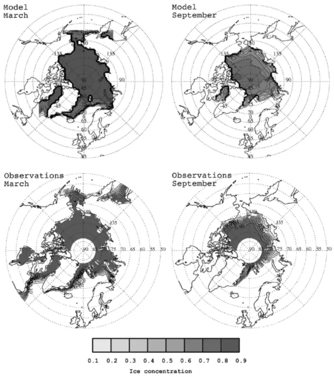
Figure 4 compares the March and September mean ice concentrations computed by the model to the corresponding observations of Comiso (1999). In March, the modeled loca-tion of the ice edge agrees relatively well with the observed one. One notes, however, that the ice cover protrudes slightly too far southward in the Barents, Greenland and Labrador Seas. In September, the simulated ice edge is somewhat south of the observed one in the Barents and Kara Seas, and ice persists in Baffin Bay, whereas observations show that this area is totally free of ice during that month. A detailed inspection of Fig. 4 also reveals that the percentage of open water within the summer pack is somewhat overestimated. However, it is worth noting that passive microwave observa-tions underestimate the ice concentration, particularly during summer where surface melt is seen by the algorithms as re-duced concentration (Steffen and Schweiger, 1991).
Although we have identified a certain number of short-comings in the results of the control run conducted with the model, the discussion above demonstrates that the model shows acceptably good agreement with enough aspects of the
seasonal behavior of the Arctic sea ice cover to permit a re-liable study of the effect of the assimilation of ice velocity and/or concentration data through twin experiments. 4.2 Thermodynamic perturbation
4.2.1 Assimilation of ice velocity data
In this section, we examine the impact of assimilating ice velocities from the TS on the model behavior when the model is thermodynamically perturbed (see Sect. 3.1).
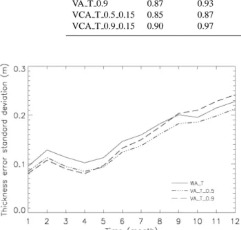
Tables 2 and 3 compare the annual mean results obtained without and with assimilation for year 1995 to the TS for dif-ferent values of the weight ku(0.3, 0.5 and 0.9). Clearly, the
assimilation of ice velocity data is a good way to improve the simulation of the ice motion. The higher ku, the
bet-ter the assimilated ice velocities. The correlations between the computed ice concentrations and thicknesses and the TS ones are also enhanced when assimilation is performed and when kuincreases. Taken together, the error in ice thickness
averaged over the entire area occupied by the pack and the standard deviation of this error are minimum for ku=0.5. As
can be seen from Fig. 5, the standard deviation of the ice thickness error is slightly smaller for ku=0.9 than for ku=0.5
during the first five months of 1995 and becomes signifi-cantly larger afterwards. According to Thorndike (1975), the dynamics seek the mean and the thermodynamics the ex-tremes. When the thermodynamic perturbation is applied to the model, thermodynamics seek an anomalous extreme in ice thickness. The model ice dynamics act to reduce this anomaly, but data assimilation defeats this process. For in-stance, if the ice is too thick in a region because of too low
Fig. 4. March (left) and September (right) ice concentrations averaged over the period 1979–1999 from the control run (top) and as observed (Comiso, 1999; bottom). The pole hole in the observations is due to lack of satellite coverage in that area. Contour interval is 0.10.
an air temperature, convergence will weaken in this area via the Kreyscher et al. (2000) correction. When higher ice ve-locities are assimilated, convergence becomes larger and ice thickens, thus defeating to lower the ice thickness error. This is especially true during summer melt and autumn freeze up. Figure 5 suggests to take ku equal to 0.5 in experiments
longer than five months. However, such a choice leads to
another problem. Table 3 indicates that the area-averaged, annual mean ice concentration bias is enhanced compared to the no-assimilation case with ku=0.5. By contrast, the error
in ice thickness is reduced, but not due to the enhancement of the ice transport. When velocity data are assimilated with ku=0.5, the velocity field after assimilation is the arithmetic
Table 2. Area-averaged, annual mean correlations between the ice velocity components from experiments WA T, VA T 0.3, VA T 0.5 and VA T 0.9 and the TS ones, and area-averaged, annual mean errors in the ice velocity components and standard deviations of these errors for experiments WA T, VA T 0.3, VA T 0.5 and VA T 0.9.
Correlation Bias (10−4m/s) Error std (m/s)
U V U V U V
WA T 0.38 0.36 2.48 −2.15 0.028 0.023
VA T 0.3 0.69 0.68 1.12 −1.09 0.018 0.015
VA T 0.5 0.84 0.83 1.25 −0.91 0.012 0.010
VA T 0.9 0.98 0.98 0.39 −0.22 0.002 0.002
Table 3. Area-averaged, annual mean correlations between the ice thickness and concentration from experiments WA T, VA T 0.3, VA T 0.5, VA T 0.9, VCA T 0.5 0.15 and VCA T 0.9 0.15 and the TS ones, and area-averaged, annual mean errors in the ice thick-ness and concentration and standard deviations of these errors for experiments WA T, VA T 0.3, VA T 0.5, VA T 0.9, VCA T 0.5 0.15 and VCA T 0.9 0.15. In experiments VCA T 0.5 0.15 and VCA T 0.9 0.15, ice thickness conservation is imposed near the ice margin and where the thermodynamic error is larger than the indirect dynamic one, and ice volume conservation is imposed everywhere else.
Correlation Bias Error std
hi Ai hi(10−2m) Ai(10−2) hi(m) Ai WA T 0.75 0.32 8.77 1.81 0.142 0.078 VA T 0.3 0.79 0.56 6.23 2.27 0.125 0.072 VA T 0.5 0.82 0.73 6.48 2.22 0.121 0.067 VA T 0.9 0.87 0.93 8.82 1.82 0.132 0.062 VCA T 0.5 0.15 0.85 0.87 −2.94 0.41 0.114 0.029 VCA T 0.9 0.15 0.90 0.97 2.82 0.38 0.100 0.023
Fig. 5. Temporal evolutions over year 1995 of the standard devi-ations of the ice thickness error for experiments WA T (solid line), VA T 0.9 (dashed line) and VA T 0.5 (dashed-dotted line).
globally smoothes the ice advection. Therefore, the ice cover experiences less divergence, which yields an enhanced ice compactness and less convergence, resulting in less ice build-up. This problem fades away as kuincreases.
As “perfect” data are assimilated into our model, one was expecting to obtain the best results with the highest weight. Our results show that this is not necessarily the case. On time scales less than five months, it seems preferable to use a large ku, while over longer time scales, a smaller kumust be used,
which generates too smooth an ice transport. 4.2.2 Assimilation of ice concentration data
Here, we evaluate the effects of the assimilation of ice con-centrations from the TS when a thermodynamic perturbation is applied to the model. In each grid cell, the sea ice volume, Vi, can be diagnosed from:
Vi =AihiS (7)
where S is the grid cell area (constant). When the ice concen-tration varies owing to assimilation, one may either conserve ice volume or ice thickness. The first solution appears more appropriate given the huge effort put in recent years into de-veloping energy-conserving sea ice models. Nonetheless, it can create serious problems. Indeed, if the ice concentration in a grid cell is too large (small) due to the use of an er-roneously low (high) surface air temperature, there is every chance that the ice thickness is also overestimated (underes-timated). This is at least true during the winter and during summer melt. The autumn freeze-up case would probably be
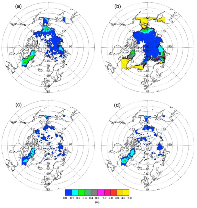
Fig. 6. Differences (in absolute value) in annual mean ice thickness for year 1996 between experiment WA T and the TS (a), and between experiment CA T 0.15 and the TS when we impose ice volume conservation everywhere (b), ice thickness conservation everywhere (c) and ice thickness conservation near the ice margin and where the thermodynamic error is larger than the indirect dynamic one, and ice volume conservation everywhere else (d).
different. The assimilation will then tend to reduce (increase) the ice concentration. If the conservation of ice volume is imposed, this will lead to an increase (decrease) in ice thick-ness, thus enhancing the initial thickness bias. Figures 6a and b display the changes (in absolute value) in annual mean ice thickness between the experiments without and with assim-ilation of ice concentration data and the TS for year 1996. In the case with assimilation, ice volume conservation is im-posed and kA=0.15. It can be seen from these figures that
the assimilation deteriorates in many places the simulation of the sea ice thickness, especially near the ice edge where the thermodynamic error can be quite large due to the high interannual variability of the air temperature.
The second solution is to conserve ice thickness. Over-all, this solution improves the ice thickness estimate com-pared to the no-assimilation case (Fig. 6c). However, the thickness bias is observed to increase along the north coast of Alaska. In several grid cells there, the applied
Fig. 7. Temporal evolutions over year 1996 of the area-averaged correlations between ice thicknesses from experiments WA T and CA T 0.15 and the TS ones (a), the area-averaged ice thickness er-rors for experiments WA T and CA T 0.15 (b), and the standard deviations of the ice thickness errors for experiments WA T and CA T 0.15 (c). In the experiment with assimilation, ice thickness conservation is imposed near the ice margin and where the ther-modynamic error is larger than the indirect dynamic one, and ice volume conservation is imposed everywhere else.
thermodynamic perturbation produces so large ice accumu-lations that there is no longer ice convergence (because of Kreyscher et al. (2000) correction) into the grid cells. Only ice divergence is allowed, which tends to decrease the ice compactness. At this stage, the dynamic error has become larger than the thermodynamic one. The assimilation of ice concentration data corrects the too low concentration by adding an ice block of thickness equal to that of the pre-existing ice, which has no effect on the ice thickness. Fur-thermore, as ice volume is not conserved in the assimila-tion process, during ice divergence episodes, the grid cells affected by this problem act as a source of ice volume for the neighboring ones. Clearly, in those specific cases, it would be better to impose ice volume conservation.
Given these results, we propose to combine the two solu-tions. Basically, the thermodynamic perturbation introduces direct thermodynamic errors into the model as well as in-direct dynamic and thermodynamic ones, due to ice thick-ness and concentration biases. Near the ice edge and in ar-eas where thermodynamic errors are greater than dynamic ones, ice thickness conservation is imperative. Elsewhere, it seems more appropriate to conserve ice volume. The prob-lem now is to draw a distinction between thermodynamic and dynamic errors. We observed that, when ice concentration in a grid cell is corrected through data assimilation, if the er-ror is of thermodynamic (dynamic) nature, the model con-centration remains close to (strongly deviates from) the TS one during the next time step. Therefore, we assume that the magnitude of the ice concentration error is an indicator of the model error type. When the difference between modeled and TS concentrations is smaller (greater) than a certain thresh-old, the error is assumed to be thermodynamic (dynamic). Figure 6d reveals that this technique further improves the simulation of the annual mean ice thickness pattern for year 1996 compared to the case where ice thickness conservation is applied everywhere. On the other hand, Fig. 7 shows that the monthly values of the area-averaged ice thickness bias and thickness error standard deviation are significantly re-duced in comparison with the no-assimilation case and that the correlation between the modeled and TS ice thicknesses is slightly enhanced.
Figure 6d indicates that, in some places, the assimilation slightly deteriorates the ice thickness estimate. This feature is mostly due to the use of thresholds in the model, such as the thickness of newly formed ice in leads, the maximum al-lowable ice concentration or Kreyscher et al. (2000) correc-tion threshold. Owing to those thresholds, small differences in the sea ice state can have noticeable effects. These effects are particularly visible during the first couple of years of sim-ulation. Afterwards, when the ice thickness error caused by the perturbed forcing grows, they become negligible and the improvement brought by data assimilation to the model be-comes clearer.
All the experiments that we conducted with the model point to the fact that choosing kA equal to 0.15 gives the
best model improvement while preventing the appearance of model instabilities. They also suggest that, because of the strong connection between ice concentration and ice thick-ness, assimilation of concentration data has to be handled with care. The best solution we found is to conserve ice thickness after assimilation near the ice margin and where the thermodynamic error is larger than the indirect dynamic one, and to conserve ice volume everywhere else. To be com-plete, the ice thickness correction should depend on the phys-ical mechanisms involved. However, ice thickness errors are seldom fully corrected and they influence the next physical mechanism errors. According to this feedback, the correc-tion suggested in this paper is one possible correccorrec-tion to be applied. This solution is therefore retained in the experiments discussed in the following section.
4.2.3 Assimilation of ice velocity and concentration data The model performance can be further enhanced by assimi-lating simultaneously ice velocities and concentrations from the TS. But, here again, the choice of the weights appears crucial.
In Table 3, we compare the annual mean results obtained without and with assimilation for year 1995 to the TS for two sets of weights: ku=0.5 and kA=0.15; ku=0.9 and kA=0.15.
For ku=0.5 and kA=0.15, the correlations between the
esti-mated ice concentrations and thicknesses and the TS ones are significantly increased, and the standard deviations of the errors in ice concentration and thickness are markedly re-duced. Nevertheless, as a result of the assimilation-induced smoothing of the ice velocity field discussed in Sect. 4.2.1, the simulated ice pack is slightly too thin and too compact. When ku=0.9 and kA=0.15, the model results seem further
improved. However, for the same reason as the one given in Sect. 4.2.1, when time goes by, the simulation of ice thick-ness progressively deteriorates. In summary, the assimilation of ice velocity and/or concentration data is able to weaken the effect of the thermodynamic perturbation applied to the model. Nonetheless, given the sensitivity of the improve-ment brought by assimilation to the weights, their value must be selected carefully as a function of the characteristic time scale of the assimilated variable, the type of model error and the model integration length.
4.3 Dynamic perturbation
4.3.1 Assimilation of ice velocity data
Here, we assess the impact of the assimilation of ice veloci-ties from the TS on the model performance when the model is dynamically perturbed (see Sect. 3.1). Several values of kv
have been tested. Table 4 shows that, for ku=0.5, the
corre-lations between the simulated ice concentrations and thick-nesses and the TS ones increase notably in 1995 compared to the no-assimilation case, and that the standard deviations
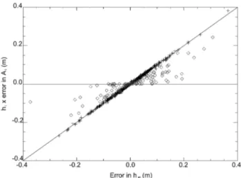
Fig. 8. Error in himversus error in Ai times hi at the end of the
first time step of experiment WA D. The diamonds correspond to the grid cells where either the modeled or TS ice concentration is equal to Amaxand the crosses correspond to the other grid cells. The 1:1 line is also plotted.
of the errors in ice concentration and thickness decrease sig-nificantly. However, once again, because of the ice velocity smoothing caused by assimilation, the model ice field be-comes somewhat too thin and too compact. The situation is much improved when ku=0.9. Actually, the best way to get
rid of this problem would be to use a weight equal to 1. 4.3.2 Assimilation of ice concentration data
In this section, we try to find the best way to assimilate ice concentrations from the TS into the model in order to im-prove the ice thickness estimate when a dynamic perturbation is applied to the model.
As already mentioned, the ice concentration is tightly linked to the ice thickness and volume. To avoid error feed-backs, we analyze ice concentration and thickness errors just after the first time step of the experiment without assimila-tion. We define the mean ice thickness in a given grid cell as him=Aihi. Figure 8 reveals that, for most grid cells, the
error in himis quasi-equal to the product of hi and the error
in Ai. As Vi=himS, this suggests that the ice volume should
be corrected by adding or removing an ice block of thickness hi and of concentration equal to the error in Ai. In other
words, the in-situ ice thickness should be conserved after as-similation of ice concentration data. This also suggests that kAshould be taken equal to 1. If this technique is used, the
error in himis reduced to almost zero in the majority of grid
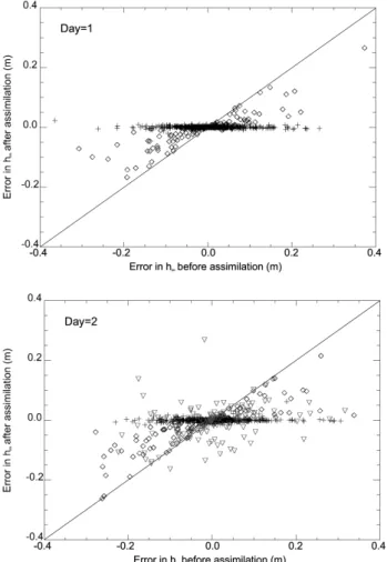
cells (crosses in Fig. 9a). Nonetheless, in grid cells where either the modeled or TS concentration is equal to the max-imum allowable value Amax(diamonds in Fig. 9a), the bias remains large. During the second time step, the assimilation of ice concentration data lowers the error in himin most grid
Table 4. Same as Table 3, but for experiments WA D, VA D 0.5, VA D 0.9, CA D 0.3 and VCA D 0.9 0.3. In experiments CA D 0.3 and VCA D 0.9 0.3, we impose ice volume conservation within the ice pack and ice thickness conservation close to the ice edge.
Correlation Bias Error std
hi Ai hi(10−2m) Ai(10−2) hi(m) Ai WA D 0.78 0.29 0.21 0.05 0.106 0.066 VA D 0.5 0.90 0.72 −3.18 0.63 0.079 0.043 VA D 0.9 0.98 0.98 −0.80 0.14 0.027 0.014 CA D 0.3 0.55 0.68 1.17 0.05 0.119 0.029 VCA D 0.9 0.3 0.92 1.00 −0.01 0.02 0.055 0.006
Fig. 9. (a) Error in himbefore assimilation versus error in himafter
assimilation for the first time step of experiment CA D 0.3. The ice thickness is assumed to be conserved during the assimilation process. (b) Same as (a), but for the second time step of experiment CA D 0.3. The diamonds correspond to the grid cells where either the modeled or TS ice concentration is equal to Amax. The triangles correspond to the grid cells where, during the previous time step, either the modeled or TS ice concentrations were equal to Amax. The crosses correspond to the other grid cells. The 1:1 line is also plotted.
worsens in grid cells where a significant bias was observed during the first time step (triangles in Fig. 9b). This behav-ior is mainly due to ice piling. The model piles the ice to prevent Ai>Amax. If ice piling occurs in the perturbed ex-periment but not in the TS, assimilation of ice concentration data is only able to partly correct the simulated ice concen-tration. On the other hand, as we suppose that hi is
con-served after assimilation, the error in hi remains, as well as
part of the error in him. Later, this error weakly perturbs the
thermodynamic component of the model and strongly affects the dynamic one, which leads to error amplification. Note that this is also true for grid cells where Ai<Amaxwhile TS
shows Ai=Amax. The proposed solution therefore seems to
work on short time scales, with initial conditions very close to reality. However, on longer time scales, it is inappropri-ate because, in problematic grid cells, it leaves errors which grow afterwards. It is worth noting that a smaller kAlowers
the error amplification process without erasing it.
Another possible solution might be to impose, after assim-ilation, ice volume conservation within the ice pack and ice thickness conservation close to the ice edge, where the mean ice thickness is less than say 0.5 m. This solution would be consistent with the best solution found for the thermodynam-ically perturbed model. However, as shown in Table 4 for kA=0.30, it deteriorates the ice thickness simulation
com-pared to the no-assimilation case. This is caused by the fact that, during a particular time step, the perturbed wind forcing greatly modifies the ice circulation and the geographical dis-tribution of ice thickness. Consequently, the next time step, the ice melt/growth rate and transport can be very different from the TS.
In conclusion, when the model is dynamically perturbed, assimilation of ice concentrations from the TS is one way to improve the estimated ice concentrations but not always the estimate of ice thickness. As a matter of fact, for short-term studies (a few days), the best model improvement is observed when in-situ ice thickness is conserved. For longer-term studies, one should rather conserve the ice volume than the in-situ ice thickness, unless the mean ice thickness is lower than 0.5 m.
4.3.3 Assimilation of ice velocity and concentration data When both ice velocities and concentrations from the TS are assimilated into the model, the abovementioned problems re-main and the model improvement is not always straightfor-ward. The best results are obtained with ku=0.9 and kA=0.3
(a kuequal to 1 would correct most of the errors without
giv-ing the chance to the concentration assimilation to operate) and when the ice volume is forced to be conserved every-where except near the ice margin. Results for year 1995 of this experiment are summarized in Table 4. The model per-formance is overall enhanced compared to the velocity-only assimilation case. Even if the average correlation between the computed ice thicknesses and the TS ones is slightly re-duced, the average ice thickness bias and the standard devia-tion of this error are drastically diminished.
5 Conclusions
Twin experiments have been conducted with a simplified model of the Arctic sea ice cover in order to determine to what extent the assimilation of ice velocity and/or concen-tration data improves the model behavior and, in particular, the simulation of ice thickness. Such experiments are ideal-ized and do not allow tackling all the problems encountered when assimilating real observations into more complex mod-els. Likewise, the data assimilation results are assumed to be model dependent and the model used here is simplified (no shear deformation, no ocean feedbacks, ...). However, this study is a first step towards real data assimilation into a more complex sea ice-ocean model and permits a detailed analysis of the way the model reacts to the data assimilation scheme. Our results show that the assimilation of ice concentra-tion data can easily lead to a deterioraconcentra-tion of the model per-formance if it is not handled with care. This is mostly due to the strong connection between ice concentration and ice thickness. The best way to estimate the sea ice state through concentration assimilation in the sea ice model is to make the distinction between model thermodynamic and dynamic errors. When the model error in a grid cell is mainly ther-modynamic or near the ice edge, the assimilation must add or remove an ice block of thickness equal to that of the pre-existing ice to better fit the observed ice concentration, which means that ice volume must not be conserved in the process. On the contrary, when the model error is mainly dynamic, the assimilation must preserve the ice volume. For our ex-perimental design, the most appropriate value for the weight, kA, is 0.15–0.3.
Assimilation of ice velocity data is found to significantly improve the overall ice model estimation if the model dy-namics is wrong, especially when a high weight is utilized. When the model error is thermodynamic, the improvement brought by assimilation is not as clear. The results obtained in the present study also reveal that the assimilation of ice
velocity data and the assimilation of ice concentration data are very complementary, so that assimilating simultaneously ice velocity and concentration data into the model seems to be the best means to enhance the ability of the model to re-produce the observed features of the sea ice field.
Data assimilation is surely a suitable method for improv-ing simulations of the sea ice pack made by large-scale sea ice models. Nevertheless, it is worth stressing that a better estimate of one model variable does not automatically yield better estimates of the other model variables. In addition, thresholds in the sea ice model can increase errors when data are assimilated. Finally, a good knowledge of both model and observation errors is also essential to apply consistent corrections.
Acknowledgements. We wish to thank Cecilia Bitz and Walt Meier
for their very constructive suggestions to improve the manuscript and Hugues Goosse, and Martin Vancoppenolle for helpful discus-sions about various aspects of this work. We also thank Xavier Fettweis for technical support. The NCEP/NCAR reanalysis data were provided by the National Oceanic and Atmospheric Administration Cooperative Institute for Research in Environ-mental Sciences Climate Diagnostics Center, Boulder, online at http://www.cdc.noaa.gov. The sea ice concentration observations were obtained through the National Snow and Ice Data Center, University of Colorado, Boulder. V. Duli`ere is supported by the Fonds pour la Formation `a la Recherche dans l’Industrie et dans l’Agriculture. This study was carried out within the scope of the project “A Second-Generation Model of the Ocean System” funded by the Communaut´e Franc¸aise de Belgique (Actions de Recherche Concert´ees, ARC 04/09-316) and the project “Contribution of the assimilation of satellite data to sea ice modeling” funded by the Universit´e Catholique de Louvain (Fonds Sp´ecial de Recherche). Edited by: A. Sterl
References
Arbetter, T., Lynch, A., Maslanik, J., and Meier, W.: Effects of data assimilation of ice motion in a basin-scale sea ice model, Ice in the Environment: Proceedings of the 16th IAHR Interna-tional Symposium on Ice, Dunedin, New Zealand, 2–6 December 2002, International Association of Hydraulic Engineering and Research, edited by: Squire, V. and Langhore, P., 3, 186–193, 2002.
Bjørgo, E., Johannessen, O., and Miles, M.: Analysis of merged SMMR/SSMI time series of Arctic and Antarctic sea ice param-eters, Geophys. Res. Lett., 24, 413–416, 1997.
Bourke, R. and Garrett, R.: Sea ice thickness distribution in the Arctic Ocean, Cold Reg. Sci. Technol., 13, 259–280, 1987. Cavalieri, D., Gloersen, P., Parkinson, J., Comiso, J., and Zwally,
H.: Observed hemispheric asymmetry in global sea ice changes, Science, 278, 1104–1106, 1997.
Cavalieri, D., Parkinson, C., and Vinnikov, K.: 30-Year satellite record reveals contrasting Arctic and Antarctic decadal sea ice variability, Geophys. Res. Lett., 30, 18, doi:10.1029/2003GL018031, 2003.
Comiso, J.: Bootstrap sea ice concentrations for NIMBUS-7 SMMR and DMSP SSM/I, National Snow and Ice Data Center, Boulder, CO, USA, digital media, 1999.
Comiso, J.: A rapidly declining perennial sea ice cover in the Arc-tic, Geophys. Res. Lett., 20, 1956, doi:10.1029/2002GL015650, 2002.
Comiso, J. and Steffen, J.: Studies of Antarctic sea ice concentra-tions from satellite data and their applicaconcentra-tions, J. Geophys. Res., 106, 31 361–31 385, 2001.
Dai, M., Arbetter, T., and Meier, W.: Data assimilation of sea-ice motion vectors: Sensitivity to the parameterization of sea-sea-ice strength, Ann. Glaciol., 44, 357–360, 2006.
Emery, W., Fowler, C., and Maslanik, J.: Satellite-derived maps of Arctic and Antarctic sea ice motion: 1988 to 1994, Geophys. Res. Lett., 24, 897–900, 1997.
Fichefet, T., Tartinville, B., and Goosse, H.: Antarctic sea ice variability during 1958–1999 : A simulation with a global ice-ocean model, J. Geophys. Res., 108(C3), 3102, doi:10.1029/2001JC001148-12, 2003.
Fowler, C. and Emery, W. and Maslanik, J.: Satellite-derived evolu-tion of Arctic sea ice ages: October 1978 to March 2003, IEEE Geoscience and Remote Sensor Letters, 1, 2, 71–74,2004. Fox, A., Haines, K., de Cuevas, B., and Webb, D.: Altimeter
assim-ilation in the OCCAM global model, Part I : A twin experiment, J. Mar. Syst., 26, 303–320., 2000.
Ghil, M. and Malanotte-Rizzoli, P.: Data assimilation in meteorol-ogy and oceanography, Adv. Geophys., 33, 141–266, 1991. Goosse, H.: Modelling the large-scale behaviour of the coupled
ocean-sea ice system, Ph.D. thesis, Universit´e Catholique de Louvain, Louvain-la-Neuve, Belgium, 1997.
Hibler: A dynamic thermodynamic sea ice model, J. Phys. Oceanogr., 9, 815–846, 1979.
Holloway, G. and Sou, T.: Has Arctic sea ice rapidly thinned?, J. Climate, 15, 1691–1701, 2002.
Kalnay, E., Kanamitsu, M., Kistler, R., Collins, W., Deaven, D., Gandin, L., Iredell, M., Saha, S., White, G., Woollen, J., Zhu, Y., Chelliah, M., Ebisuzaki, W., Higgins, W., Janowiak, J., Mo, K., Ropelewski, C., Wang, J., Leetmaa, A., Reynolds, R., Jenne, R., and Joseph, D.: The NCEP/NCAR 40-year reanalysis project, B. Am. Meteor. Soc., 77(3), 437–471, 1996.
K¨oberle, C. and Gerdes, R.: Mechanisms determining the variabil-ity of the Arctic sea ice conditions and export, J. Climate, 16, 2843–2858, 2003.
Kreyscher, M., Harder, M., Lemke, P., and Flato, G.: Results of the Sea Ice Model Intercomparison Project : Evaluation of sea ice rheology schemes for use in climate simulations, J. Geophys. Res., 105, 11 299–11 320, 2000.
Kwok, R., Zwally, H., and Yi, D.: ICEsat observations of Arctic sea ice: a first look, Geophys. Res. Lett., 31, 16, doi:10.1029/2004GL020309, 2004.
Laxon, S., Peacock, N., and Smith, D.: High interannual variability of sea ice thickness in the Arctic region, Nature, 425, 947–950, 2003.
Lin, C.-L., Chai, T., and Sun, J.: Retrieval of flow structures in a convective boundary layer using an adjoint model : identical twin experiments, J. Atmos. Sci., 58, 1767–1783, 2001. Lindsay, R. and Zhang, J.: The thinning of Arctic sea ice, 1988–
2003: have we passed a tipping point?, J. Climate, 18, 4879– 4894, 2005.
Lindsay, R. and Zhang, J.: Assimilation of ice concentration in an ice-ocean model, J. Atmos. Oceanic Technol., 23, 742–749, 2006.
Lindsay, R., Zhang, J., and Rothrock, D.: Sea ice deformation rates from measurements and in a model, Atmos.-Oceans, 40, 35–47, 2003.
Lisaeter, K., Rosanova, J., and Evensen, G.: Assimilation of ice concentration in a coupled ice-ocean model, using the Ensemble Kalman Filter, Ocean Dyn., 53, 368–388, 2003.
Maslowski, W., Newton, B., Schlosser, P., Semtner, A., and Martin-son, D.: Modeling recent climate variability in the Arctic Ocean, Geophys. Res. Lett., 27, 3743–3746, 2000.
McPhee, M.: An analysis of pack ice drift in summer, in: Sea Ice Processes and Models, edited by: Pritchard, R. S., Univ. Wash. Press, Seattle, pp. 62–75, 1980.
Meier, W. and Maslanik, J.: Synoptic-scale ice-motion case-studies using assimilated motion fields, Ann. Glaciol., 33, 145–150, 2001a.
Meier, W. and Maslanik, J.: Improved sea ice parcel trajectories in the Arctic via data assimilation, Mar. Pollut. Bull., 42, 506–512, 2001b.
Meier, W. and Maslanik, J.: Effect of environmental conditions on observed, modeled, and assimilated sea ice motion errors, J. Geo-phys. Res., 108, 21.1–21.11, 2003.
Meier, W., Maslanik, J., and Fowler, C.: Error analysis and assim-ilation of remotely sensed ice motion within an Arctic sea ice model, J. Geophys. Res., 105, 3339–3356, 2000.
Parkinson, C. and Washington, W.: A large-scale numerical model of sea ice, J. Geophys. Res., 84, 311–337, 1979.
Parkinson, C., Cavalieri, D., Gloersen, P., Zwally, H., and Comiso, J.: Arctic sea ice extents, areas, and trends, 1978–1996, J. Geo-phys. Res., 104, 20 837–20 856, 1999.
Perovich, D. and Grenfell, T. and Richter-Menge, J. and Light, B. and Tucker III, W. and Eicken, H.: Thin and thinner: sea ice mass balance measurements during SHEBA, J. Geophys. Res., 108(C3), 8050, doi:10.1029/2001JC001079, 2003.
Rigor, I. and Wallace, J.: Variations in the age of Arctic seaice and summer seaice extent, Geophys. Res. Lett., 31, L09401, doi:10.1029/2004GL019492, 2004.
Rothrock, D. and Zhang, J.: Arctic Ocean sea ice volume: What ex-plains its recent depletion?, J. Geophys. Res., 110(C1), C01002, doi:10.1029/2004JC002282, 2005.
Rothrock, D. and Zhang, J. and Yu, Y.: The Arctic ice thick-ness anomaly of the 1990s: A consistent view from ob-servations and models, J. Geophys. Res., 108(C3), 3083, doi:10.1029/2001JC001208, 2003.
Rothrock, D., Yu, Y., and Maykut, G.: Thinning of the arctic sea-ice cover, Geophys. Res. Lett., 26, 3469–3472, 1999.
Semtner, A.: A model of the thermodynamic growth of sea ice in numerical investigations of climate, J. Phys. Oceanogr., 6, 379– 389, 1976.
Smolarkiewicz, P.: A simple positive definite advection scheme with small implicit diffusion, Mon. Wea. Rev., 111, 479–486, 1983.
Steele, M., Morley, R., and Ermold, W.: PHC: A global ocean hydrography with a high quality Arctic Ocean, J. Climate, 14, 2079–2087, 2001.
Steffen, H. and Schweiger, A.: Nasa team algorithm for sea ice concentration retrieval from Defense Meteorological Satellite Program Special Sensor Microwave Imager: Comparison with Landsat Imagery, J. Geophys. Res., 96, 21 971–21 987, 1991. Thomas, D. and Rothrock, D.: Blending Sequential Scanning
Mul-tichannel Microwave Radiometer and buoy data into a sea ice model, J. Geophys. Res., 94, 10 907–10 920, 1989.
Thomas, D. and Rothrock, D.: The Arctic ocean ice balance : a Kalman smoother estimate, J. Geophys. Res., 98, 10 053–10 067, 1993.
Thomas, D., Martin, S., Rothrock, D., and Steele, M.: Assimilating satellite concentration data into an Arctic sea ice mass balance model, J. Geophys. Res., 101, 20 849–20 868, 1996.
Thorndike, A.: A naive zero-dimensional sea ice model, J. Geo-phys. Res., 93, 5 093–5 099, 1975.
Timmermann, R., Goosse, H., Madec, G., Fichefet, T., Ethe, C., and Duliere, V.: On the representation of high latitude processes in the ORCALIM global coupled sea ice-ocean model, Ocean Model., 8, 175–201, 2005.
Trenberth, K., Olson, J., and Large, W.: A global ocean wind stress climatology based on the ECMWF analyses, Tech. rep., National Center for Atmospheric Research Technical Note 338, 1989.
Tucker, W., Weatherly, J., Eppler, D., Farmer, D., and Bentley, D.: Evidence for rapid thinning of sea ice in the western Arctic Ocean at the end of the 1980s, Geophys. Res. Lett., 28, 2851– 2854, 2001.
Weaver, R., Steffen, K., Heinrichs, J., Maslanik, J., and Flato, G.: Data assimilation in sea-ice monitoring, International Glaciology Society, 31, 327–332, 2000.
Winsor, P.: Arctic sea ice thickness remained constant during the 1990s, Geophys. Res. Lett., 28, 1039–1041, 2001.
Yu, Y. and Maykut, G. and Rothrock, D.: Changes in the thickness distribution of the Arctic sea ice between 1958– 1970 and 1993–1997, J. Geophys. Res., 109, C08004, doi:10.1029/2003JC001982, 2004.
Yu, Y. and Lindsay, R.: Comparisons of thin ice fractions estimated from RGPS and AVHRR, J. Geophys. Res., 108(C12), 3387, doi:10.1029/2002JC001319, 2003.
Zhang, J., Thomas, D., Rothrock, D., Lindsay, R., and Yu, Y.: As-similation of ice motion observations and comparisons with sub-marine ice thickness data, J. Geophys. Res., 108, 1–18, 2003.