HAL Id: hal-02506644
https://hal.archives-ouvertes.fr/hal-02506644
Submitted on 12 Mar 2020
HAL is a multi-disciplinary open access
archive for the deposit and dissemination of
sci-entific research documents, whether they are
pub-lished or not. The documents may come from
teaching and research institutions in France or
abroad, or from public or private research centers.
L’archive ouverte pluridisciplinaire HAL, est
destinée au dépôt et à la diffusion de documents
scientifiques de niveau recherche, publiés ou non,
émanant des établissements d’enseignement et de
recherche français ou étrangers, des laboratoires
publics ou privés.
flow with very low submergence
Yulia Akutina, Olivier Eiff, Frédéric Moulin, Maxime Rouzès
To cite this version:
Yulia Akutina, Olivier Eiff, Frédéric Moulin, Maxime Rouzès. Lateral bed-roughness variation in
shallow open-channel flow with very low submergence. Environmental Fluid Mechanics, Springer
Verlag, 2019, pp.1339-1361. �10.1007/s10652-019-09678-w�. �hal-02506644�
OATAO is an open access repository that collects the work of Toulouse
researchers and makes it freely available over the web where possible
Any correspondence concerning this service should be sent
to the repository administrator:
[email protected]
This is a publisher’s version published in:
http://oatao.univ-toulouse.fr/24268
To cite this version:
Akutina, Yulia and Eiff, Olivier and Moulin, Frédéric Y. and
Rouzès, Maxime Lateral bed-roughness variation in shallow
open-channel flow with very low submergence. (2019)
Environmental Fluid Mechanics. 1-12. ISSN 1567-7419
Official URL:
https://doi.org/10.1007/s10652-019-09678-w
ORIGINAL ARTICLE
Lateral bed‑roughness variation in shallow open‑channel
flow with very low submergence
Yulia Akutina1 · Olivier Eiff1 · Frédéric Y. Moulin2 · Maxime Rouzes2
Received: 5 April 2018 / Accepted: 14 March 2019 © The Author(s) 2019
Abstract
Quantifying turbulent fluxes and secondary structures in shallow channel flows is impor-tant for predicting momentum and mass transfer in rivers as well as channel capacity and associated water levels. Here, we focus on the flow over a lateral bed-roughness variation with very low relative submergence of the roughness elements, h∕k = {3, 2, 1.5} , where h is the flow depth and k is the roughness height. Measurements were performed in a 1.1 m wide and 26 m long glass flume whose bed was fitted with cubes arranged in two regular side-by-side patterns with frontal densities 𝜆f= 0.2 and 0.4 to create a rough-to-rougher
variation. Measurements were performed using stereoscopic PIV in two orthogonal planes, in a vertical transverse plane spanning the two roughness types, and in a longitudinal one at the interface between the roughness types. The results show that the bulk velocity dif-ference between the two sides of the channel increases with decreasing h/k. Also, contrary to what is observed at high relative submergence with smooth-to-rough transitions, higher bulk velocities occur on the side with higher roughness. This difference is increasing as the flow becomes shallower and is shown to be due to increasing effective depths ratios, lead-ing to increaslead-ingly lower friction factor ratios with lower friction factors on the high-veloc-ity but rougher side. Although increasing streamwise momentum transfer at the interface is needed as h/k decreases, the turbulent and secondary circulation transfer of momentum is increasingly inhibited. A globally-driven secondary-circulation at h∕k = 3 ceases for lower
h/k and roughness-scale circulation becomes dominant. Also, even the increased global
shear does not lead to large-scale Kelvin Helmholtz instabilities structures. However, the relative importance of the roughness difference on the flow is augmented as the flow becomes shallower and momentum transfer due to lateral dispersive stresses increases.
Keywords Open-channel flow · Shallow flow · Lateral roughness variation · Low relative submergence · Secondary currents · Stereoscopic PIV
* Olivier Eiff [email protected]
1 Institute for Hydromechanics, Karlsruhe Institute of Technology, Karlsruhe, Germany 2 Institut de Mécanique des Fluides de Toulouse, Université de Toulouse, CNRS-INPT-UPS,
Environmental Fluid Mechanics
1 Introduction
It is common that river beds have a lateral variation in roughness, shall that be vegetation on one side of the channel or a change in grain size on the bed. During high floods, the flows over the floodplains are almost always spatially inhomogeneous. In order to predict water levels in a river or over the floodplains one needs to calculate the flow capacity of the channel. The channel capacity for a uniform bed structure over a given cross-section of a channel is a function of the resistance imposed by the channel bed but is also influenced by the lateral transfer of momentum driven by lateral gradients at the edges. Indeed, it is com-mon to model inhomogeneous beds with different roughness coefficients, suggesting that a flow that has two different roughnesses on two sides is equivalent to two streams flowing parallel to each other as if they were separated by a frictionless wall. However, neglecting the effects resulting from the interaction between the two streams may result in an overesti-mation of the channel capacity.
Another important characteristic of shallow flows over floodplains is the low relative submergence of the roughness elements, for instance for an urbanised floodplain during an extreme flood where buildings may be submerged. Even for homogeneous beds, one can expect the boundary-layer approach to fail [15], although experiments over a bed of cubes have shown that the logarithmic law still prevails if the double-averaged velocities are con-sidered [24].
Open-channel flows with lateral variations have been studied under diverse conditions: shallow mixing layers, where the flow is characterized by a lateral velocity difference with no roughness changes [2, 4, 26]; smooth-to-rough roughness variation due to compound channels, where the lateral velocity difference is driven mainly by the difference in the flow depth [6, 14, 21, 22, 27]; and finally, the most directly relevant case, flows with lateral transition between completely smooth and rough beds [3, 17, 28] and between smooth and vegetation patches [12, 19, 30]. Rough-to-rougher transitions, however, have to our knowl-edge not yet been considered.
As discussed by Vermaas et al. [28] in the context of smooth-to-rough lateral transitions, there are three main mechanisms governing the lateral exchange of streamwise momentum: (1) secondary currents, (2) turbulent flux resulting from the shear between the two parallel flows with different velocities, and (3) bulk transfer. When the flow is fully developed, the bulk transfer is negligible.
Secondary currents or circulations driven by a lateral difference in bed roughness (smooth-rough transition) was first observed by Studerus [25]. Vermaas et al. [28] showed that this secondary current becomes more important in terms of its contribution to the lat-eral exchange of streamwise momentum with increasing water depth. Their h/k ratios on the rough side ranged from about 10 to 30, i.e., standard submergence where flow resist-ance formulations based on the logarithmic law are generally considered to hold. Low sub-mergence ( h∕k < 10 , where h is the flow depth and k is the roughness height) or very low submergence ( h∕k < 3 ) or rough-to-rough transitions were not considered.
Turbulent momentum transfer can be realized through different mechanisms. Large-scale turbulent coherent structures originating from a Kelvin–Helmholtz type shear insta-bility have been studied in plane shallow mixing layers by Chu and Babarutsi [4], Chen and Jirka [2], Uijttewaal and Booij [26]. These studies concluded that the growth of the shear layer is suppressed by the bottom friction and therefore, the exchange due to coher-ent turbulcoher-ent structures is reduced for smaller depths, higher roughness and lower velocity difference between the parallel flows. On the other hand, Proust et al. [23] showed that in
a compound channel, where the velocity difference is sustained by the difference in the flow depth, the coherent structures persist even for very shallow conditions. Proust et al. [23] proposed that these structures are controlled only by the difference in the bulk veloci-ties over the flood plain, U2, and the main channel, U1, expressed as a velocity ratio (also
referred to as dimensionless shear), 𝜆 = (U1− U2)∕(U1+ U2) . For 𝜆 > 0.3 , large-scale
tur-bulent structures were observed provided the presence of an inflection point in the mean longitudinal velocity profile.
Turbulent exchange in wall-bounded flows in general is also controlled by large- and very-large-scale motions. These have received considerable attention in canonical wall flows [11, 13, 16]. In a river, they were studied by Franca and Lemmin [10] and in a rough-bed laboratory open-channel by Cameron et al. [1]. These structures consist of streaks of higher and lower streamwise velocities and associated vortices. Nezu and Nakagawa [18] observed that the characteristic width of the streaks in an open channel is twice the water depth. Wang et al. [29] showed that they grow linearly coming up to the free surface. How-ever, according to Defina [5], the streaks tend to disappear for low relative submergence, when h∕ks<2 , where ks is the equivalent sand-roughness.
Thus, it appears that a variety of phenomena can be expected for lateral rough-to-rougher transitions under very low relative submergence ( h∕k < 3 ) and it is not clear which. The roughness elements themselves are expected to play a growing role as the flows become shallower (decreasing h/k) since the roughness sublayer increasingly dominates the flow depth [24]. Whether analogies can be drawn with flows with higher relative submer-gence or flows with a smooth-to-rough lateral transition will be investigated in this paper.
2 Methodology
The flow measurements were carried out in the Environmental Fluid Mechanics laboratory of the Institut de Mécanique des Fluides de Toulouse (IMFT). The flows were generated in a 26 m long glass flume with a width 2B = 1.1 m and a slope of 0.3%. The flow parameters were chosen such that a quasi-uniform flow was achieved in the measurement area within 1% of the flow-depth variation. The bed roughness was modeled with cubes with a side of
k= 0.02 m arranged in regular patterns. The lateral variation in the roughness between the two sides of the bed was realized by a difference in roughness frontal density, 𝜆f = h2∕L1L2
(see Fig. 1). 𝜆f is equal to 0.4 on the left-hand side (referred to as S2 roughness type) and
0.2 on the right-hand side (referred to as S1). The experiments were performed for three flow cases with varying relative submergence, h∕k = {3, 2, 1.5} (Table 1). The streamwise, lateral and vertical directions are respectively defined as the (x, y, z) coordinates, where
x= 0 is taken at the channel entry (after the inlet tank), y = 0 in the midplane of the chan-nel and z = 0 on the bottom of the cubes. The rough bed extends from 2.6 m ≤ x ≤ 24 m. The three velocity components (u, v, w) were measured via stereoscopic PIV at x = 19.2 m in a vertical cross-plane spanning the two roughness types (green line on Fig. 1) and in a longitudinal plane at y = 0.01 m (red line in Fig. 1). The y = 0.01 m position was chosen since it corresponds to the centre of the row of cubes belonging to the edges of the S1 and S2 patterns, i.e., the geometric interface. The images were recorded using two high-resolution ( 2560 × 2160 px) 14-bit sCMOS cameras LaVisionEdge, resulting in a spatial resolution of about 9, 11 and 15 Kolmogorov length scales for h∕k = {3, 2, 1.5} , respec-tively [24]. For both planes, the cameras were positioned on the side of the flume with glass prisms fixed to the glass walls whereas the laser sheet arrived collimated from below
Environmental Fluid Mechanics Fig . 1 Sc hematic of t he s ter eoscopic PIV se t-up in t he c hannel (t op vie w). The measur ements w er e t ak en in a v er tical cr oss-flo w plane (g
reen line) spanning t
he tw
o
bed-roughness types, and in t
he longitudinal plane (r ed line) positioned at t he g eome trical centr e of t he flume. The fr ont al densities of S2 and S1 ar e 𝜆f = 0 .4 on t he lef t (S2), and 𝜆f = 0 .2 on t he r ight-hand side (S1)
through transparent cubes in order to avoid fanning shadows. 11,000 stereo image pairs were acquired for each experimental run at a frequency of 10 Hz for a duration of 18 min, ensuring adequate time-convergence with about 9000–18,000 bulk time units. The veloc-ity fields were calculated using the software DaVis by LaVision. More detail on the flow generation and stereoscopic set-up can be found in Rouzes et al. [24] who analyse the flow in the center of the S1 bed.
3 Results
3.1 Mean flow3.1.1 Lateral distribution of streamwise velocity and bed friction
The time-averaged velocities obtained from the stereoscopic PIV measurements in the transverse plane are given in Fig. 2b–d, corresponding to the three relative submergences,
h∕k = {3, 2, 1.5} , respectively. The streamwise velocity is shown as a colormap and the in-plane velocities as vectors. In the case of the higher relative submergence, h∕k = 3 , the streamwise velocity distribution is relatively homogeneous in the lateral direction with a local decrease around y ≈ 0.02 m, while for h∕k = 1.5 the position of the cubes determines the distribution of the streamwise velocity all the way up to the free surface, in agreement with the roughness sublayer heights for S1 estimated in Rouzes et al. [24]. Also, the mean streamwise velocity is notably higher over S1 (right-hand side), especially for the two shal-lowest flows, h∕k = 2 and 1.5. This trend can be seen even clearer in Fig. 2a which presents the time- and depth-averaged streamwise velocity profiles ⟨u⟩z(y) normalized by the time
and (y, z)-averaged value ⟨u⟩yz (given in Table 1). The trend suggests that decreasing
rela-tive submergence augments the importance of the roughness difference between the paral-lel flows and increases the difference between the bulk flow on the two sides.
The three normalized ⟨u⟩z(y)∕⟨u⟩yz profiles intersect very closely to the geometric
inter-face at ⟨u⟩z(y)∕⟨u⟩yz≈ 1 . The three measured bulk velocities above the canopy ⟨u⟩yz (given
in Table 1) are therefore good estimates of the interface velocities.
Table 1 also gives the bulk velocity Uk defined classically by Uk= Q∕Ak where
Ak= 2B(h − k) is the cross-sectional area above the canopy. It also gives Ue = Q∕Ae
Table 1 Flow conditions for the three sets of experiments with varying relative submergence, h/k, where
h is the flow depth (measured from the bottom of the flume), k is the roughness height and Q is the total
discharge
Three different bulk velocities across the total channel width (2B) are defined: (1) Uk= Q∕Ak where
Ak= 2B(h − k) , i.e., the cross-sectional area above the canopy, (2) Ue= Q∕Ae with an effective cross-sectional area given by Ae= B(de,1+ de,2) where de,1 and de,2 are the effective depths based on the volu-metric displacement of the cubes. (3) ⟨u⟩yz is the temporally and spatially averaged streamwise veloc-ity in the transverse measurement plane across the interface over the canopies (see Fig. 2 below).
Frk= Uk∕ √
g(h − k) is the Froude number associated with Uk
h/k Q (l/s) Uk (cm/s) Frk Ue (cm/s) ⟨u⟩yz (cm/s)
3 15.8 35.8 0.58 26.5 35.1
2 5.2 23.6 0.53 13.9 20.9
Environmental Fluid Mechanics
where Ae= B(de,1+ de,2) is computed with effective flow depths on each side. The
effec-tive depths are given by de,i= h − k(1 − 𝜙i ) considering the volumetric displacement by
the cubes with 𝜙i= Vf ,i∕Vt being the porosity of the beds ( 𝜙i= {0.8, 0.6} for S1 and S2,
respectively). As expected, these bulk velocities are lower than Uk , reflecting the larger
effective crosssectional flow area. They are also lower than ⟨u⟩yz reflecting the contribution
of the lower velocity canopy flow.
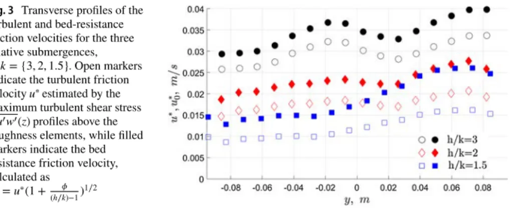
Figure 3 shows the lateral profile of the turbulent friction velocity u∗ (open markers).
At each location, u∗ is estimated by first averaging the turbulent shear-stress profiles in
Fig. 2 a Time- and depth-averaged profiles of streamwise velocity for three relative submergences, h/k. The horizontal red lines denote the elevated effective bed-level considering the blockage by the cubes, defining the effective flow depths de,i . b–d Time-averaged streamwise (color) and cross-plane (vectors) velocities at the vertical cross-section ( x = 19.2 m) for the three flow conditions with varying relative submergence,
h∕k = {3, 2, 1.5} . For the vertical component of the vectors, the spatially averaged vertical velocity has been subtracted (see Sect. 3.1.2). Dashed lines indicate the position an thickness of the longitudinal plane. The vectors are plotted every third grid point
the y-direction across half a roughness length k and then taking the maximum of the resulting profiles just above the roughness elements. This method is more robust than an extrapolation to the top of the elements as done in homogeneous flows since extrapola-tion is not straightforward to apply with non-linear shear stress profiles. It should be noted that u∗ at the top of the canopy is the velocity scale which scales the turbulence [9,
20] which is lower than the friction velocity associated with the bed shear stress. The total shear-stress acting on the bed (the bed resistance) is given by the friction velocity
u∗ 0= u
∗(1 + 𝜙
(h∕k)−1)
1∕2 (see [20]) and is also shown in Fig. 3 (filled symbols). Clearly, for
smaller h/k, the difference between the two shear velocities increases.
It can be seen in Fig. 3 that both friction velocities are higher over the S1 rough-ness pattern (right-hand side). Computation of the equivalent sand-roughrough-ness, ks (not
shown), via logarithmic law fits (see [24], for the method) also confirms that S1 is rougher than S2 for the h/k range investigated, following the u∗ y-variation tendency.
Hence, the bed-resistance, u∗
0 , the turbulence scale, u
∗ , and the roughness scale, k
s , are
all globally higher on S1 than on S2. Yet, the flow is faster over S1, especially for the lowest relative submergence (see Fig. 2d), implying that the bulk flow over the surface with higher equivalent sand-roughness (S1) is higher.
Bulk flow quantities for both sides are given in Table 2 (for S1 with i = 1 and for S2 with i = 2 ). The flow rates on S1, Q1 , were estimated by integrating the velocity profiles
measured in the center of S1 above the canopy by Rouzes et al. [24]. To account for the
Fig. 3 Transverse profiles of the
turbulent and bed-resistance friction velocities for the three relative submergences,
h∕k = {3, 2, 1.5} . Open markers indicate the turbulent friction velocity u∗ estimated by the maximum turbulent shear stress −u�w�(z) profiles above the roughness elements, while filled markers indicate the bed resistance friction velocity, calculated as u∗ 0= u ∗(1 + 𝜙 (h∕k)−1) 1∕2
Table 2 Estimated bulk flow parameters Xi for the two roughness sides S1 ( i = 1 ) and S2 ( i = 2 ), as well as
the ratios of the parameters X1∕X2
de,i are the effective water depths, Qi the total flow rates, Ue,i the associated bulk velocities, u∗0,i the
bed-resistance friction velocities (for S1 from Rouzes et al. [24] in the center of S1 and for S2 estimated from Fig. 3) h/k S1 ( i = 1) S2 ( i = 2) X1∕X2 3 2 1.5 3 2 1.5 3 2 1.5 Xi= de,i (cm) 5.6 3.6 2.6 5.2 3.6 2.6 1.08 1.12 1.18 Qi (l/s) 9.2 3.5 1.5 6.5 1.7 0.5 1.4 2.1 2.8 Ue,i (cm/s) 29.7 17.8 10.3 22.8 9.4 4.3 1.3 1.9 2.4 u∗ 0,i (cm/s) 4.3 3.3 2.5 3.8 2.4 1.8 1.14 1.35 1.42 fi 0.16 0.27 0.48 0.22 0.52 1.38 0.75 0.51 0.35
Environmental Fluid Mechanics
flow within the canopy, the canopy profiles measured by Florens [8] for same bed and
h∕k = 3 were used. Then Q2= Q − Q1. The bulk velocities Ue,i= Qi∕Ae,i were computed
with the effective water depths de,i , i.e., with Ae,i= Bde,i.
In agreement with the transverse-plane measurements above the canopy in Fig. 2, higher bulk velocities Ue,i are found on the rougher side (S1) for all h/k. This is the
opposite of what one expects from smooth-to-rough transitions with high submergence [28] or from recent experiments with very low submergence ( h∕k ≤ 2 ) with the same S1 configuration on the rough side [7].
The apparent contradiction can be explained by the different effective flow depths de,i
on the two sides which are higher on the S1 side for all h/k investigated (see Table 2). Their ratio de,1∕de,2 , also given in Table 2, increases with decreasing relative submergence,
following the bulk-velocity ratio Ue,i trend. The effective depth ratios are evidently high
enough for all h/k to compensate the higher bed stress over S1. This is confirmed by the bulk Darcy friction factors for both sides, fi= 8u∗0,i
2
∕U2
e,i which are higher on the smoother
S2 side, increasingly so as h/k decreases.
In summary, for very low relative submergence, the effect of geometrically increasing effective flow depth with a lower-density roughness pattern becomes more important than the associated increase in roughness length and bed shear-stress. This dominating flow-depth effect increases as the relative submergence decreases. Inversely, as seen in Table 2, for increasing h/k, all depth, flow-rate, bulk-velocity and friction-factor ratios approach 1 for some h∕k > 3 , so that the roughness effect is expected to dominate again for higher h/k, with lower bulk velocities on the rougher side as usually expected. For a smooth-to-rough transition, the effective depth is always higher on the smooth side (at least when the obsta-cles on the rough side sit above the level of the smooth bed) so that even for h∕k < 3 , both the effective depth and roughness are favorable to slower bulk flow on the rougher side, as observed in Dupuis et al. [7].
3.1.2 Secondary currents
For the highest relative submergence ratio investigated ( h∕k = 3 ), a counterclockwise sec-ondary current can be identified in Fig. 2b. It is centred around y ≈ 0.01 m, i.e., at the geometric interface between the two roughness types. The secondary current appears to be similar to the one observed at the interface between the smooth and rough surfaces in Vermaas et al. [28]. Also as in Vermaas et al. [28] or the classical secondary flow results reviewed in Nezu and Nakagawa [18], the current ascends over the high bulk velocity side (S1) and descends over the low bulk velocity side (S2). The sense of rotation is also in accordance with the local variation of u∗
0 seen in Fig. 3 around y ≈ 0, with u ∗
0 being locally
higher on the downward side (S2). The global y-variation of u∗
0 , however, is in the opposite
direction, i.e., rougher on the S1 side. The size of the recirculation zone suggests it scales with the water depth and so appears to be driven by the global bulk velocity gradient.
In the intermediate case of h∕k = 2 (Fig. 2c), a similar secondary current appears further out at y ≈ 0.02 m. It is not, however, clear whether it is associated with the global gradi-ent or with a given roughness elemgradi-ent, since similar circulations take place at other lateral positions (e.g., at y ≈ − 0.01 and 0.07 m). Similar observations can be made for h∕k = 1.5 (Fig. 2d). To help clarify this point, we consider the longitudinal measurement plane. Fig-ure 4a–f show the time-averaged transverse and vertical velocities for all three h/k ratios, respectively. It can be seen that for h∕k = 3 and 2 the secondary current is persistent in the
Fig . 4 T ime-a ver ag ed tr ansv
erse (column 1) and v
er tical (column 2) v elocities at t he longitudinal plane at t he inter face be tw een S1 and S2 ( y = 0 .0 1 m) f or t he t hr ee flo w con -ditions wit h v ar ying r elativ e submer gence, h ∕ k ={ 3 , 2 , 1 .5 } . The tw o do
tted lines indicate t
he e xtent of t he tr ansv erse measur ement plane
Environmental Fluid Mechanics
streamwise direction and does not depend considerably on the roughness elements, while for h∕k = 1.5 , the secondary current appears only at the position of the cubes and hence is controlled solely by the roughness elements. Rouzes et al. [24] who analyzed the flow in the center of the S1 side in the same facility showed that the roughness sublayer for
h∕k = 1.5 extends all the way to the free surface of the flow. It therefore appears that for lowest relative submergence, the secondary currents are not driven by the gradient between the different roughness types, but rather by the local roughness gradients of the roughness sublayer which takes over the whole depth of the flow.
It should be noted that in Fig. 4d–f, the mean vertical velocity at the x-position of the transverse measurement plane (between the dashed lines) is directed downwards through-out the measured water depth above the cubes. This downward flow is compensated by upward flow further downstream in the wake of the cube. Since a net downward component washes out the topology of the vector fields, the net vertical velocity (time-, depth-, and width-averaged), equal to 0.13, 0.16 and 0.23 of u∗ for h∕k = {3, 2, 1.5} , respectively, was
subtracted from the time-averaged vertical velocity field in Fig. 2b–d. This allows to better visualize the secondary flow patterns.
3.1.3 Vertical vorticity
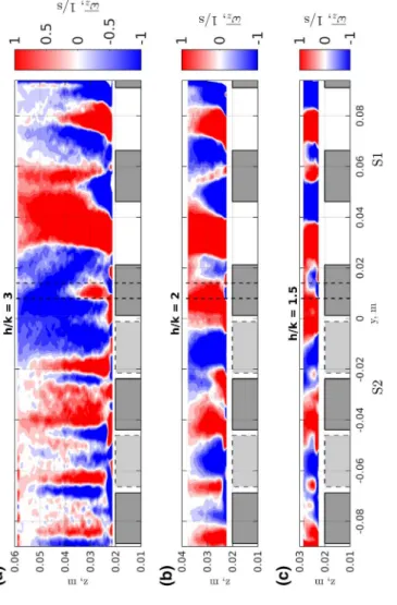
More evidence of the roughness-scale influence versus the global variation is seen in the mean vertical vorticity fields in the transverse plane. The time-averaged vertical vorticity,
𝜔z , is presented in Fig. 5a–c for all three submergence ratios. Here, 𝜔z is calculated from
the three-dimensional velocity fields of the transverse plane measurements, u(t, y, z) and
v(t, y, z), using Taylor’s “frozen turbulence” hypothesis to convert the time coordinate t into x= tu (justified by the relatively low turbulence intensity levels in this advective flow).The plots show that mean vertical vorticity is generally in phase with the roughness elements. For h∕k = 3 , however, a large negative vertical vorticity patch can be seen whose width is of the order of the water depth and is therefore not directly associated with the roughness scale. The width corresponds to the scale of a local change in the transverse gradient of the streamwise velocity, the signature of which can be observed in Fig. 3. It is also in agree-ment with depth-averaged streamwise velocity profiles presented in Fig. 2a. At the position of the longitudinal plane ( y = 0.01 m) the dominant sign of 𝜔z is different for h∕k = 3 than
for h∕k = 2 . The positive vorticity for h∕k = 2 appears to be local and associated with the roughness element. Such a local roughness influence can also be observed for h∕k = 1.5.
It is worth noting in Fig. 5a–c that the time-averaged vertical vorticity has a tendency to form vertical columns with alternating sign. These types of structures are not readily apparent in the instantaneous fields. It is hypothesized that the vertical structures are the result of averaging the preferential position of larger vortical structures oscillating around the roughness elements, or are the result of averaging small-scale intense vortices shed from the cubes. The origin of this phenomenon needs more investigation, but it is notable that a deeper flow in this case shows more vertical homogeneity than the shallower one.
Fig . 5 T ime-a ver ag ed v er tical v or ticity , 𝜔z , f or t he t hr ee flo w conditions wit h v ar ying r elativ e submer gence, h ∕ k ={ 3 , 2 , 1 .5 }
Environmental Fluid Mechanics
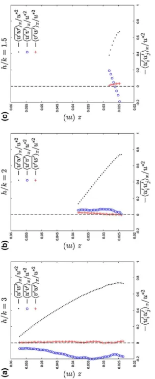
Fig
. 6
T
ime- and longitudinall
y a ver ag ed shear s tresses − ⟨ ui uj ⟩x ∕ u ∗ 2 ( y = 0 .0 1 ) f or t he t hr ee flo w conditions wit h v ar ying r elativ e submer gence, h ∕ k ={ 3 , 2 , 1 .5 }
3.2 Turbulent stresses and structures 3.2.1 Turbulent stresses
The time- and longitudinally averaged (over one pattern length) Reynolds shear stresses, −⟨u�w�⟩
x , − ⟨u�v�⟩x , and − ⟨v�w�⟩x , normalized by u∗2 (Table 3), are plotted in Fig. 6a–c for
the three relative submergences. Clearly, the vertical shear stress, − ⟨u�w�⟩
x∕u∗2 , is still the
strongest turbulent flux, as expected. One can notice a convex curvature in − ⟨u�w�⟩
x∕u∗2 ,
which indicates the presence of a secondary current [18]. Over a smooth-to-rough transi-tion as considered in Nezu and Nakagawa [18], a convex shape of the vertical shear stress is observed on the upward flow side (smooth) whereas here the flow is downward on the locally smoother side. However, the circulation agrees if the bulk velocity gradient is con-sidered, i.e., upward flow on the faster side.
The turbulent flux − ⟨v�w�⟩
x∕u∗2 is almost negligible for all the relative submergences,
implying that there is a negligible lateral transfer of vertical momentum by lateral veloc-ity fluctuations. The transverse flux of the streamwise momentum, − ⟨u�v�⟩
x∕u∗2 , on
the other hand, is seen to be not negligible, in particular for h∕k = 3 where its sign sug-gests that 𝜕⟨u⟩z∕𝜕y should be negative, which is indeed the case since 𝜕⟨u⟩z∕𝜕y changes
its sign locally due to the presence of the secondary current (see Fig. 2a). For h∕k = 2 , −⟨u�v�⟩
x∕u∗2 is positive, consistent with 𝜕⟨u⟩z∕𝜕y > 0 . However, it becomes much smaller
in magnitude compared to h∕k = 3 . In the case of h∕k = 1.5 , − ⟨u�v�⟩
x changes sign with
flow depth so that the vertically and horizontally averaged flux would be close to zero. Therefore, the net turbulent transverse flux across the y = 0 plane can be seen to decrease with increasing shallowness.
However, this decrease does not necessarily mean that turbulent intensities in the verse direction are low. In fact, the longitudinal-plane-averaged turbulence levels of trans-verse velocity component are almost as high ( vrms∕u∗= 1.14–1.36) as those of the
stream-wise one ( urms∕u∗= 1.52 − 1.70 ), see Table 3. Also, the normalized by the bulk velocities
transverse turbulence intensity levels, vrms∕⟨u⟩yz , increase with decreasing relative
submer-gence, implying that turbulent diffusivity in the transverse direction increases in the shal-lower flows (Table 3). Yet, this is due to roughness-scale effects, not the roughness frontal-density transition.
Table 3 Turbulence
characteristics for three relative submergences, h∕k = {3, 2, 1.5} , where u∗ is the streamwise-averaged friction velocity at the interface obtained from longitudinal plane, urms is the streamwise, vrms—the transverse, and wrms—the vertical r.m.s. velocities
Angle brackets, ⟨⋅⟩xz∕yz , denote averaging either in the xz or yz plane
h∕k = 3 h∕k = 2 h∕k = 1.5 u∗ (m/s) 0.036 0.024 0.016 ⟨urms⟩xz∕u∗ 1.52 1.61 1.70 ⟨urms⟩xz∕⟨u⟩yz 0.15 0.18 0.21 ⟨urms⟩yz∕⟨u⟩yz 0.12 0.12 0.15 ⟨vrms⟩xz∕u∗ 1.14 1.26 1.36 ⟨vrms⟩xz∕⟨u⟩yz 0.12 0.14 0.17 ⟨vrms⟩yz∕⟨u⟩yz 0.09 0.10 0.15 ⟨wrms⟩xz∕u∗ 0.87 0.87 0.89 ⟨wrms⟩xz∕⟨u⟩yz 0.09 0.10 0.11 ⟨wrms⟩yz∕⟨u⟩yz 0.06 0.06 0.06
Environmental Fluid Mechanics
3.2.2 Kelvin–Helmholtz instability
With decreasing relative submergence, the difference in the redistribution of the streamwise momentum increases (Fig. 2). According to Proust et al. [23] for compound channels, when the ratio based on the bulk velocities of the two sides 𝜆 = (U1− U2)∕(U1+ U2) > 0.3 ,
large-scale turbulent structures with a vertical axis of rotation develop due to Kelvin–Helmholtz shear instability. Here, taking the effective bulk velocities Ue,i , 𝜆 = {0.16, 0.44, 0.70} for
h∕k = {3, 2, 1.5} , respectively, suggesting that h∕k = 2 and 1.5 could be subject to the Kel-vin–Helmholtz shear instability. A sufficient condition for it to appear is an inflection point in the streamwise velocity profile. However, the distribution of the mean momentum in the current set-up does not resemble a classic shear-layer profile, but rather possesses numerous inflection points due to the direct roughness influence (Fig. 2a). It is thus not clear whether Kelvin–Helmholtz type vortices are expected. In order to investigate this further, auto- and cross-correlations are considered.
Figure 7 shows the temporal autocorrelation function of the transverse velocity fluc-tuations, Rt
yy , normalized by the bulk time scale, Tb= He∕⟨u⟩yz where He= h − k . The
three plots show the autocorrelation at flow depth z∕He= 0.9 for three lateral positions,
y= {− 0.075, 0.02, 0.08} m, corresponding to two positions away from the interface and at the flow interface between the roughness types (see Fig. 2). It can clearly be seen that the auto-correlation of the transverse velocity fluctuations at the interface is not greater than that away from the interface, giving the first indication of the absence of large-scale Kelvin–Helmholtz structures. Second, one expects some quasi-periodicity in the autocorrelation function if large-scale coherent structures were generated in the shear layer, but there appears none. Third, the largest turbulent time-scales at the interface are of the same order of magnitude as the bulk time scale (the graphs reach zero correlation at about 2–2.5 Tb ; a rough estimate of the integral
scale which would be about half, i.e., 1–1.2 Tb ), much shorter than large-scale
Kelvin–Helm-holtz structures. These observations include the shallowest case ( h∕k = 1.5 ) where 𝜆 > 0.3. To identify the scale of turbulent structures in the transverse direction, transverse spatial cross-correlations are computed. Fig. 8a–c shows the cross-correlation function of transverse velocity fluctuations in transverse direction,
where 𝜉 is the distance from the given starting points ( y = {− 0.075, 0.02, 0.08} m and
z= 0.9He ). The width of the cross-correlation function can be seen as a measure of the characteristic width of the turbulent structures appearing in the flow, here normalized by the effective flow depth, He . It is evident, that when normalized by He , the spatial extent
of the structures is the smallest for the h∕k = 3 , approximately 2He . As the flow becomes
shallower, their relative size increases up to 3–4 He for h∕k = 1.5 . This indicates that the
structures scale with the effective flow depth for the deeper flow, while for h∕k = 1.5 they are no longer determined by the flow depth, but rather by the roughness scale, which is much larger than the flow depth (the size of the roughness pattern is about 4He for the
shal-lowest flow). The width of the correlation function does not differ much for h∕k = 3 for dif-ferent lateral positions in the channel. For h∕k = 2 and 1.5, the structures are much larger over S1 than over S2, which again confirms the growing importance of the roughness ele-ments or scale with decreasing submergence, while giving no indication of presence of large-scale Kelvin–Helmholtz structures at the interface. The Proust criterion of 𝜆 > 0.3
Ryyy(𝜉) = ⟨v �(y, z, t)v�(y + 𝜉, z, t) ⟩t √ ⟨v�(y, z, t)2⟩ t √ ⟨v�(y + 𝜉, z, t)2⟩ t ,
05 10 15 0 0.05 0.1 0.15 0.2 R yy t Over S2 (a) 05 10 15 At the interface (b) 05 10 15 Over S1 (c) Fig . 7 T em por al aut ocor relation of t he tr ansv erse v elocity fluctuations, R t , at tyy hr ee tr ansv erse positions, y = {− 0 .0 75 , 0 .0 2 , 0 .0 8} m, and flo w dep th z∕ He = 0 .9 ; f or t he t hr ee flo w conditions wit h v ar ying r elativ e submer gence, h ∕ k ={ 3 , 2 , 1 .5 } . Tb = He ∕⟨ u⟩ yz is t
he bulk time scale. The functions ar
e a ver ag ed in v er tical and tr ansv erse dir ection o ver an ar ea of 3 b y 3 g rid points
Environmental Fluid Mechanics -2 -1 012 0 0.2 0.4 0.6 0.8 1 R yy y Over S2 (a) -2 -1 01 2 Interface (b) -2 -1 01 2 Over S1 (c) Fig . 8 Cr oss-cor relation functions of tr ansv erse v elocity fluctuations in tr ansv erse dir ection at t hr ee tr ansv erse positions, y =− 0 .0 75 , 0.02 and 0.08 m, and flo w dep th z∕ He = 0 .9 for h ∕ k ={ 3 , 2 , 1 .5 }
developed for compound channels is evidently not confirmed. This could be due to differ-ent configurations, yet the effective depth differences also act like a compound channel. Also the estimations of the relevant velocities might differ. Yet, the results are in agreement with the increasing dominance of the roughness-sublayer structures for very low h/k sug-gesting that decreasing h/k even further, and thereby increasing 𝜆 , would not lead to large-scale Kelvin–Helmholtz structures at the interface.
3.2.3 Velocity streaks
In the previous subsection, the autocorrelation function of transverse velocity fluctuations was considered to determine the presence of lateral-shear driven large-scale Kelvin–Helm-holtz structures. Now, to examine nominally vertical-shear driven boundary-layer struc-tures, we consider the autocorrelation of the streamwise velocity fluctuations (Fig. 9a–c) at the same positions. It is clear from the graphs that the characteristic time scale of the streamwise fluctuations is much larger than that of the transverse component (Fig. 7a–c). It varies between 8 Tb and 25Tb , where Tb= He∕Ubulk is the bulk time scale. This suggests
that these high correlations are associated with streamwise velocity streaks characteristic of boundary-layer structures, despite the very low submergences.
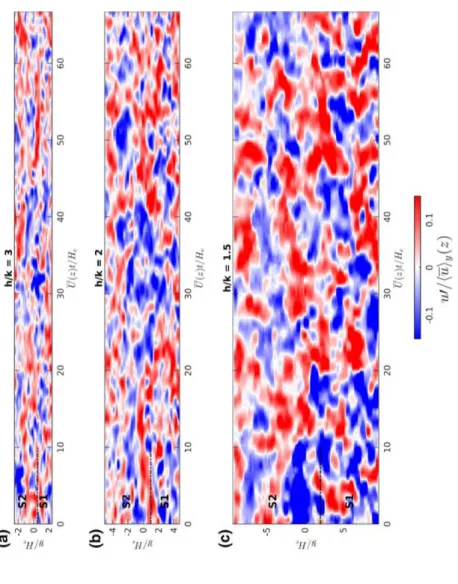
To examine the spatial organization of what appears to be streaks, Fig. 10a–c show the streamwise velocity fluctuations in the horizontal (x, y) plane, computed using Tay-lor’s “frozen turbulence” hypothesis, for the three different h/k ratios, respectively. For all three h/k, the streamwise velocity fluctuations are plotted at the same relative flow depth of z∕He= 0.81 . Velocities faster than the mean are given in red, and slower ones in blue.
For the deeper flow ( h∕k = 3 ), the structures appear elongated, as streaks characteristic of boundary-layer flows and are of the scale of about 10He . This scale is consistent with the
scale from the autocorrelation function Rt
xx . Their length appears to be just a bit longer on
S1, again consistent with Rt
xx . In the shallowest case ( h∕k = 1.5 ), the structures are smaller.
The “streaks” that now appear as “blobs” have the scale of about 5He on the S2 side and
somewhat longer over S1. For the intermediate submergence ( h∕k = 2 ) the streaks are much longer over S1 reaching about 20He . This is not so clear when viewing one snapshot
only, but can also be seen in the autocorrelation in Fig. 9.
One can also observe in Fig. 10 that the intensity of the streaks is lower on the S2 side for lower relative submergence, in particular for h∕k = 1.5 and somewhat for h∕k = 2 , while for the deeper case the intensities appear more homogeneous in the lateral direction. Therefore, as the flow becomes shallower, the flow structures or velocity streaks change their structure or cease to exist as was also observed by Defina [5]. Also, the two sides of the channel (S1 and S2) become detached at the transition and the flow over each side is then controlled by the local shape of the roughness elements. This is consistent with the absence of large-scale shear structures.
3.3 Bulk lateral transfer of streamwise momentum
The bulk lateral transfer of streamwise momentum across the interface which contributes to the momentum balance of both sides of the flow includes a contribution by secondary flows, by the lateral turbulent shear stress and, in the case of developing flows, a contribu-tion via bulk mass transfer [28]. These terms are evaluated at the interface and depth-aver-aged. Here, due to the dominance of the roughness elements, leading to periodic variations of the mean and turbulence statistics along one roughness pattern length, all transfer terms
Environmental Fluid Mechanics 01 02 03 04 05 0 0 0.05 0.1 0.15 0.2 R xx t Over S2 (a) 01 02 03 04 05 0 At the interface (b) 01 02 03 04 05 0 Over S1 (c) Fig . 9 T em por al aut ocor relation of t he str eam wise v elocity fluctuations, R t , at txx hr ee transv erse positions, y =− 0 .0 75 , 0 .0 2 and 0.08 m, f or the t hr ee flo w conditions wit h var ying r elativ e submer gence, h ∕ k = 3 , 2 and 1. Tb = He ∕⟨ u⟩ yz is t
Fig
. 10
S
tream
wise v
elocity fluctuations plo
tted on a hor izont al plane ( z∕ He = 0 .8 1 ) using T ay lor ’s “F rozen turbulence” h ypo thesis f or t he t hr ee r elativ e submer gences, h ∕ k ={ 3 , 2 , 1 .5 } . Bo th ax es ar e nor malized b y t he effectiv e flo w dep th, He
Environmental Fluid Mechanics
also need to be averaged in the streamwise direction along one pattern length. This spatial averaging leads to dispersive shear stresses which also need to be taken into account in the net momentum transfer across the interface. With spatial averaging along the x-direction (one pattern length), the contribution describing the lateral transfer by secondary flows is given by
where Vbulk= 𝜌 h∫
h
0⟨v⟩xdz= 0 for developed flow. The turbulent momentum flux is given
by
and the dispersive flux is given by
where ̃u and ̃v are the spatial velocity fluctuations defined as the time and spatially averaged velocity minus the time-averaged one, ̃u = ⟨u⟩x− u.
These fluxes were estimated by the longitudinal plane measurements above the canopy and therefore do not account for the mean, turbulent and dispersive fluctuations within the canopy. The results are presented in Table 4.
The fluxes due to the secondary currents and dispersive stresses are positive in agree-ment with the global velocity gradient with higher bulk velocities on the S1 side (see Fig. 2a) as well as the velocity gradients and corresponding flux found by Vermaas et al. [28]. The turbulent flux, however, appears to follow the local velocity gradient at least for
h∕k = 3 where it is negative. Nevertheless, the sum of the three fluxes is positive for all
h/k. It can also be seen in Table 4 that both Tsf∕𝜌u∗2 and Ttm∕𝜌u∗2 generally decrease with
decreasing relative submergence. This is surprising at first as one expects stronger positive transfer for lower h/k since the friction factors and bulk velocities ratios increase (Table 2). However, Td∕𝜌u∗2 increases more significantly with decreasing h/k suggesting that the
decreasing transfer due to secondary and turbulent motions is overtaken by the dispersive motions caused by the roughness elements. The net sum of the fluxes is highest for h∕k = 2 rather than for h∕k = 1.5 , an inconsistency showing that the neglected fluctuations below the measurement plane are significant and need to be accounted for to obtain a full balance. Apart from this inconsistency, the decreasing role of the turbulent shear with increasing
Tsf =1 h∫ z=h z=0 −𝜌⟨u⟩x(⟨v⟩x− Vbulk)dz, Ttm= 1 h∫ z=h z=0 −𝜌⟨u�v�⟩ xdz, Td= 1 h∫ z=h z=0 −𝜌⟨̃ũv⟩xdz,
Table 4 Characteristics of the lateral transfer of streamwise momentum, where Tsf∕𝜌u∗2 is the transfer due
to secondary flows, Ttm∕𝜌u∗2 is the transfer due to turbulence and Td∕𝜌u∗2 is the transfer due to dispersive stresses
h∕k = 3 h∕k = 2 h∕k = 1.5
Tsf∕𝜌u∗2 0.22 0.17 0.07
Ttm∕𝜌u∗2 − 0.14 0.05 0.01
submergence is in agreement with the absence of large-scale shear-instabilities and the decreasing role of the secondary flows is in agreement with the transition from globally driven secondary currents to roughness driven ones. On the other hand, the increasing dynamic role of the roughness elements leads to increasing dispersive stresses evidently dominating the other lateral transfer mechanisms, at least above the canopy. Below the can-opy, one can surmise that dispersive stresses also play a role, perhaps even a leading one.
4 Conclusion
Stereoscopic PIV was performed in an open-channel flow with a lateral bed-roughness var-iation and very low relative submergence ( h∕k ≤ 3 ). Two measurement planes were con-sidered at the interface between the two bed-roughness configurations, a transverse plane spanning the two roughness types and crossing the interface and a longitudinal one close to the interface. The data from the transverse plane allowed to investigate the secondary currents appearing at the border between the two parallel flows, while the data from the longitudinal plane provided space-averaged statistics at the interface. The findings can be summarized as follows.
For the investigated shallow flows, higher bulk velocities are observed over the rougher surface (S1), the surface with higher friction velocities and with higher equivalent sand-roughness lengths. Also, with decreasing relative submergence h/k from 3 to 1.5, the ratio of the bulk velocity increases, from 1.3 to 2.4. Higher bulk velocities on the rougher side are in contrast with smooth-to-rough transitions where the bulk velocity is higher over the smooth side, whether for deeper flows with h∕k > 3 [28], or for shallower low-sub-mergence flows as in the current work [6, with h∕k ≤ 2 ]. The apparent contradiction can be explained by the difference in the effective flow depths associated with the different porosities of the two roughness types. The effective flow depth is higher for the rougher pattern (S1) which is simply the byproduct of the lower porosity ( 𝜙 ). The friction factors which depend on the ratio of the friction velocity to the bulk velocity when defined by the effective depth are indeed, for all h/k, lower on the fast side (S1), as for the smooth side in smooth-to-rough transitions. The disparity between the effective-depth and roughness effects increases as h/k decreases, leading to increasingly higher velocities and lower fric-tion factors on the rougher side, relative to the smoother side. Inversely, it can be surmised that for some h∕k > 3 , the roughness effect becomes larger than the effective-depth one so that the bulk velocity is again higher on the smoother side (S2).
The increasing velocity ratio as h/k decreases has to be balanced by an increase in the streamwise momentum transfer across the interface. For developed flows, this can be achieved by turbulent shear stress, mean secondary flow, or, in particular for low-sub-mergence situations as proposed here, by dispersive stresses. Yet, even though the global transverse gradients of the streamwise velocity are higher for the shallower cases, the local gradients due to the roughness elements increasingly dominate at lower h/k. Accordingly, large-scale Kelvin–Helmholtz type structures are not observed by the correlation analy-ses, even for the strongest lateral shear at h∕k = 1.5 , and are not expected to do so for even lower h/k. Also, the two sides show increasingly independent boundary layers struc-tures (streaks). Consistently, the lateral turbulent flux − 𝜌⟨u�v�⟩
xz across the interface also
decreases with lower h/k and is attributable only to the relatively weak local transverse gradients of the streamwise velocity at this interface, controlled by the local roughness pat-tern. Similarly, a global-scale secondary current is only observed for h∕k = 3 , while for
Environmental Fluid Mechanics
h∕k = 2 and 1.5 the secondary currents associated with the roughness elements become predominant. The decrease in strength of the turbulent and secondary flow fluxes in spite of a necessarily increasing net flux is counteracted by the strengthening of the dispersive effects associated with the roughness elements. The lateral dispersive stress, − 𝜌⟨̃ũv⟩xz ,
grows more than twice with decreasing h/k.
In summary, the behavior of the interaction of the flows between the two rough sides is markedly dependent on the relative submergence for low submergence conditions. The bulk velocity gradient is opposite of what is observed for smooth-to-rough transitions and what can be expected for higher submergence flows ( h∕k > 3 ). Turbulent shear stresses and secondary flows controlled by the global shear as observed at high submergence, in par-ticular for smooth-to-rough transitions or at the interfaces of compound channels, become unimportant. Instead, turbulent shear and secondary flows are increasingly controlled by the roughness-scale as the flows become shallower. To allow the increasing total momen-tum flux from the smoother side to the rougher as the flow becomes shallower, the disper-sive stresses, also driven by the roughnesses, are increasing. For a full momentum balance, however, velocity measurements at the interface including within the canopy are necessary.
Acknowledgements This work was supported by EC Hydralab IV/PISCES project (Grant Number 261520)
and by the ANR FlowRes project (Grant Number 14-CE03-0010). M. Rouzes benefited during his PhD from financial support by the Direction Générale de l’Armement (DGA). The help in the experimental set-up by S. Cazin, M. Marchal and S. Font is gratefully acknowledged.
Open Access This article is distributed under the terms of the Creative Commons Attribution 4.0
Interna-tional License (http://creat iveco mmons .org/licen ses/by/4.0/), which permits unrestricted use, distribution, and reproduction in any medium, provided you give appropriate credit to the original author(s) and the source, provide a link to the Creative Commons license, and indicate if changes were made.
References
1. Cameron S, Nikora V, Stewart M (2017) Very-large-scale motions in rough-bed open-channel flow. J Fluid Mech 814:416–429
2. Chen D, Jirka GH (1997) Absolute and convective instabilities of plane turbulent wakes in a shallow water layer. J Fluid Mech 338:157–172
3. Choi SU, Park M, Kang H (2007) Numerical simulations of cellular secondary currents and suspended sediment transport in open-channel flows over smooth-rough bed strips. J Hydraul Res 45(6):829–840 4. Chu VH, Babarutsi S (1988) Confinement and bed-friction effects in shallow turbulent mixing layers. J
Hydraul Eng 114(10):1257–1274
5. Defina A (1996) Transverse spacing of low-speed streaks in a channel flow over a rough bed. Coherent flow structures in open channels. Wiley, London, pp 87–99
6. Dupuis V, Proust S, Berni C, Paquier A (2017) Mixing layer development in compound channel flows with submerged and emergent rigid vegetation over the floodplains. Exp Fluids 58(4):30
7. Dupuis V, Moulin F, Cazin S, Marchal M, Elyakime P, Barron JP, Eiff O (2018) Shallow flow over a bed with a lateral change of roughness. In: Proceedings of the international conference on fluvial hydraulics (River Flow 2018). Lyon-Villeurbanne, France, 5–8 September
8. Florens E (2010) Couche limite turbulente dans les écoulements à surface libre: étude expérimentale d’effets de macro-rugosités. PhD thesis, Université de Toulouse, France
9. Florens E, Eiff O, Moulin F (2013) Defining the roughness sublayer and its turbulence statistics. Exp Fluids 54:1500
10. Franca M, Lemmin U (2005) Cross-section periodicity of turbulent gravel-bed river flows. In: Proceed-ings of the 4th IAHR symposium on river, coastal, and estuarine morphodynamics (RCEM 2005), Urbana, Illinois, USA, 4–7 October, vol 1, pp 203–10
11. Guala M, Hommema SE, Adrian RJ (2006) Large-scale and very-large-scale motions in turbulent pipe flow. J Fluid Mech 554:521–542
12. Han L, Zeng Y, Chen L, Huai W (2016) Lateral velocity distribution in open channels with partially flexible submerged vegetation. Environ Fluid Mech 16(6):1267–1282
13. Hutchins N, Marusic I (2007) Evidence of very long meandering features in the logarithmic region of turbulent boundary layers. J Fluid Mech 579:1–28
14. Kara S, Stoesser T, Sturm TW (2012) Turbulence statistics in compound channels with deep and shal-low overbank fshal-lows. J Hydraul Res 50(5):482–493
15. Katul G, Wiberg P, Albertson J, Hornberger G (2002) A mixing layer theory for flow resistance in shallow streams. Water Resour Res 38(11):1250
16. Kim K, Adrian R (1999) Very large-scale motion in the outer layer. Phys Fluids 11(2):417–422 17. Kimura I, Uijttewaal W (2014) Computations on lateral momentum transfer on roughness transition in
shallow open channel flows. J Jpn Soc Civ Eng (JSCE) 2(1):159–167
18. Nezu I, Nakagawa H (1993) Turbulence in open channel flows. IAHR monographs. Taylor & Francis, London
19. Perucca E, Camporeale C, Ridolfi L (2009) Estimation of the dispersion coefficient in rivers with riparian vegetation. Adv Water Resour 32(1):78–87
20. Pokrajac D, Finnigan JJ, Manes C, McEwan I, Nikora V (2006) On the definition of the shear velocity in rough bed open channel flows. In: Proceedings of the international conference on fluvial hydraulics (River Flow 2006), Lisbon, Portugal, vol 1, pp 89–98
21. Proust S, Bousmar D, Rivière N, Paquier A, Zech Y (2010) Energy losses in compound open channels. Ad Water Resour 33(1):1–16
22. Proust S, Fernandes JN, Peltier Y, Leal JB, Riviere N, Cardoso AH (2013) Turbulent non-uniform flows in straight compound open-channels. J Hydraul Res 51(6):656–667
23. Proust S, Fernandes JN, Leal JB, Riviere N, Peltier Y (2017) Mixing layer and coherent structures in compound channel flows: effects of transverse flow, velocity ratio and vertical confinement. Water Resour Res 53(4):3387–3406
24. Rouzes M, Moulin F, Florens E, Eiff O (2018) Low relative-submergence effects in a rough-bed open-channel flow. J Hydraul Res 57(2):139–166
25. Studerus FX (1982) Sekundärströmungen im offenen gerinne über rauhen längsstreifen. PhD thesis, ETH Zurich
26. Uijttewaal W, Booij R (2000) Effects of shallowness on the development of free-surface mixing layers. Phys Fluids 12(2):392–402
27. Van Prooijen BC, Battjes JA, Uijttewaal WS (2005) Momentum exchange in straight uniform com-pound channel flow. J Hydraul Eng 131(3):175–183
28. Vermaas DA, Uijttewaal WSJ, Hoitink AJE (2011) Lateral transfer of streamwise momentum caused by a roughness transition across a shallow channel. Water Resour Res 47(2):W02530
29. Wang H, Zhong Q, Wang X, Li D (2017) Quantitative characterization of streaky structures in open-channel flows. J Hydraul Eng 143(10):04017040
30. White BL, Nepf HM (2007) Shear instability and coherent structures in shallow flow adjacent to a porous layer. J Fluid Mech 593:1–32
Publisher’s Note Springer Nature remains neutral with regard to jurisdictional claims in published maps and