HAL Id: pastel-00666690
https://pastel.archives-ouvertes.fr/pastel-00666690
Submitted on 6 Feb 2012
HAL is a multi-disciplinary open access
archive for the deposit and dissemination of sci-entific research documents, whether they are pub-lished or not. The documents may come from teaching and research institutions in France or abroad, or from public or private research centers.
L’archive ouverte pluridisciplinaire HAL, est destinée au dépôt et à la diffusion de documents scientifiques de niveau recherche, publiés ou non, émanant des établissements d’enseignement et de recherche français ou étrangers, des laboratoires publics ou privés.
exchanges in the urban atmosphere
Yongfeng Qu
To cite this version:
Yongfeng Qu. Three-dimensional modeling of radiative and convective exchanges in the urban at-mosphere. Earth Sciences. Université Paris-Est, 2011. English. �NNT : 2011PEST1111�. �pastel-00666690�
ÉCOLE DES PONTS PARISTECH / UNIVERSITÉ PARIS-EST
P H D T H E S I S
to obtain the title of
PhD of the Université of Paris-Est
Specialty : S
CIENCE
, E
NGINEERING AND
E
NVIRONMENT
Defended by
Yongfeng QU
Three-dimensional modeling of radiative
and convective exchanges in the urban
atmosphere
Provisional date of defense: November 18, 2011
Jury :
Reviewers : Dr. Majorie MUSY - CERMA
Dr. Valéry MASSON - Météo-France
Examinators : Pr. Jean François SINI - École Centrale de Nantes
Pr. Jean Philippe GASTELLU-ETCHEGORRY - CESBIO
Pr. Marina K.A. NEOPHYTOU - University of Cyprus
Dr. Patrice G. MESTAYER - IRSTV
Advisor : Dr. Bertrand CARISSIMO - CEREA
Co-advisor : Dr. Maya MILLIEZ - CEREA
Acknowledgments
This research was conducted with the financial support from EDF. I thank Grégoire Pigeon for providing access to the CAPITOUL data and the Defense Threat Reduction Agency (DTRA) for providing access to the MUST data.
I would like to express my gratitude to my advisor, Bertrand Carissimo, for his insight-ful suggestions and guidance. More particularly, I must thank my co-advisor, Maya Milliez, whose endless patience, good-natured helpfulness, throughout kept the thesis on track and sub-stantially improved it at every stage. I would like also to recognize the contribution of my co-advisor Luc Musson-Genon who gave me invaluable advice and provided me administra-tive assistance on numerous occasions.
I would like to express my sincere gratitude to Majorie Musy and Valéry Masson who take precious time off from their tight schedule to be reviewer. I am also greatly indebted to Jean-François Sini, Jean Philippe Gastellu-Etchegorry, Patrice Mestayer and Marina Neophytou to be the jury committee members.
My thanks go also to Christian Seigneur, Director of the CEREA, for hosting me in his laboratory. Thanks to all the CEREA members who have instructed and helped me a lot in the past three years. Also thanks to the personel of the university of Paris-Est and doctoral School for their kind support.
I am also grateful to the department MFEE of EDF R&D for hosting me in Chatou and for providing the facilities to conduct this thesis.
I would also like to acknowledge the CERMA laboratory for their technical assistance on the SOLENE software, especially, Julien Bouyer and Laurent Malys.
I am greatly indebted to people for their many helpful suggestions and comments: Richard Howard, Alexandre Douce, Namane Méchitoua, David Monfort, Patrice Mestayer, Majorie Musy, James Voogt, Jörg Franke, Marina Neophytou, Bert Blocken, Dominique Groleau.
Special thanks go to my friends and colleges who have supported me throughout my re-search: Denis Wendum, Dominique Demengel, Eric Gilbert, Eric Dupont, Raphael Bresson,
Cédric Dall’ozzo, Fanny Coulon, Venkatesh Duraisamy, Marie Garo and Hanane Zaïdi and many others.
There is not enough space, here, to mention all the people who have helped me, with scien-tific discussions, or with their friendship and encouragement, during this thesis work. I would like to thank all of them.
Contents
1 Context and objectives 1
1.1 Background . . . 1
1.1.1 Urban heat island . . . 2
1.1.2 Air quality . . . 3
1.1.3 Energy management . . . 3
1.1.4 Pedestrian wind comfort . . . 4
1.2 Urban physics . . . 5
1.2.1 Spatial and temporal scales and urban boundary layer . . . 5
1.2.2 Urban energy balance . . . 8
1.3 Objectives and structure of the thesis . . . 12
2 Model design 15 2.1 General CFD modeling approach for the urban environment . . . 15
2.1.1 Best practice guidelines . . . 18
2.1.2 Mesh issues . . . 27
2.2 Review of some Urban Energy Balance Models . . . 32
2.2.1 Urban Energy Balance Modeling. . . 32
2.2.2 International Urban Energy Balance Models Comparison . . . 35
2.3 A new coupled radiative-dynamic 3D scheme in Code_Saturne for modeling urban areas . . . 38
2.3.1 Presentation of the atmospheric module in Code_Saturne . . . 39
2.3.2 3D Atmospheric Radiative model . . . 42
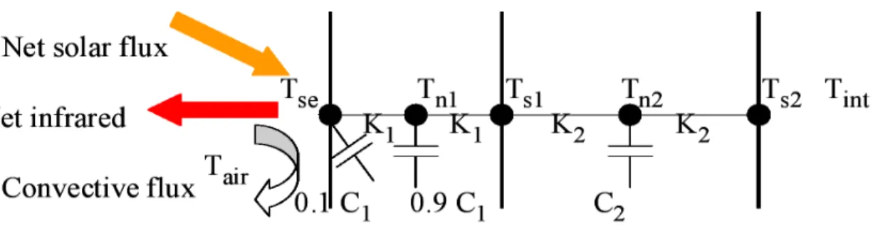
2.3.3 Surface temperature models . . . 47
3 Micrometeorological modeling of radiative and convective effects with a building resolving code: published in Journal of Applied Meteorology and Climatology,
(2011) 50, 1713–1724 53
4 A comparison of two radiation models: Code_Saturne and SOLENE 67
4.1 Introduction . . . 67
4.2 Description of SOLENE model . . . 70
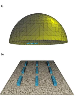
4.2.1 Geometry and mesh . . . 70
4.2.2 Thermo-radiative model . . . 72
4.3 Radiation analyses . . . 74
4.3.1 Set-up for radiation computation . . . 74
4.3.2 Comparison of direct solar flux. . . 75
4.3.3 Comparison of diffuse solar flux . . . 77
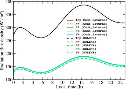
4.3.4 Comparison of long-wave radiation flux . . . 80
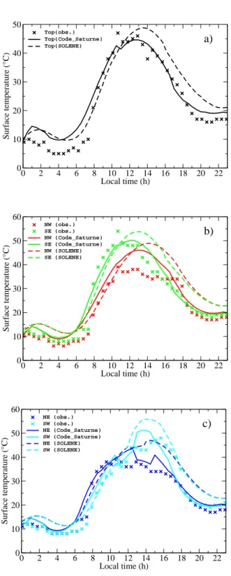
4.3.5 Comparison of surface temperatures . . . 81
4.4 Conclusions and perspectives . . . 82
5 Numerical study of the thermal effects of buildings on low-speed airflow taking into account 3D atmospheric radiation in urban canopy: paper submitted to Jour-nal of Wind Engineering & Industrial Aerodynamics 87 6 Validation with CAPITOUL field experiment 120 6.1 Introduction . . . 121
6.2 Overview of CAPITOUL field experiment . . . 121
6.2.1 Objectives and description of the site . . . 122
6.3 Simulation set-up . . . 126
6.3.1 Choice of the computational domain . . . 127
6.3.2 Mesh strategy . . . 127
Contents v
6.4 Results and discussion . . . 131
6.4.1 Comparison of IRT pictures . . . 131
6.4.2 Comparison of the local diurnal evolution of brightness surface tem-perature Tbr . . . 138
6.4.3 Model-Observation comparison of heat fluxes . . . 139
6.4.4 Model-Observation comparison of friction velocity u∗ . . . 144
6.4.5 Statistical comparison with hand-held IRT data . . . 147
6.5 Conclusions and perspectives . . . 153
7 Conclusions and Future Work 155 7.1 Summary and Conclusions . . . 155
7.2 Perspectives . . . 158
C
HAPTER
1
Context and objectives
Contents
1.1 Background . . . . 1
1.1.1 Urban heat island . . . 2
1.1.2 Air quality . . . 3
1.1.3 Energy management . . . 3
1.1.4 Pedestrian wind comfort . . . 4
1.2 Urban physics . . . . 5
1.2.1 Spatial and temporal scales and urban boundary layer . . . 5
1.2.2 Urban energy balance . . . 8
1.3 Objectives and structure of the thesis . . . . 12
1.1
Background
Urbanization is a sign of modernization, industrialization and mobilization. It implies for a transformation in the social environment, political organization and division of work. On the other hand, rapid urban extension in the last century had far-reaching consequences for sus-tainability and had profoundly changed the environment by everyday activities. Furthermore, more than half of the world’s population live in urban areas. As described byOke(1987), the process of urbanization produces radical changes in the nature of the surface and atmospheric
properties of a region. It involves the transformation of the radiative, thermal, hydrology and aerodynamic characteristics and thereby alters the natural energy and hydrology balances, as well as the wind and turbulence levels.
Therefore, among the many issues and challenges involved in urban development, are the environment ones, such as:
• Urban heat island • Air quality
• Pedestrian wind comfort • Energy management
1.1.1
Urban heat island
The Urban Heat Island (UHI) phenomenon consists in an increased air temperature within cities in comparison to the rural surroundings. It was first identified by Howard (1820) over the city of London. Especially at night, the air temperature difference can reach 3 to 10 K for large agglomerations (Oke,1987). The deterioration of the urban thermal environment has been recognized as a serious problem during the summer months even in mid-latitude regions. During heat waves, it can lead to serious consequences in terms of public health. This was revealed during a important heat wave in August 2003 that affected Europe and caused more than 70, 000 victims, with a majority in urban areas (15, 000 in France) (Hémon and Jougla,
2003). This deterioration could become worse in the context of climate change (temperature increase even larger in cities due to a positive feedback) (McCarthy et al.,2010).
Consequently, urban development initiatives that consider the influence on the urban mal environment have received more attention than they have in the past. In addition, a ther-mally comfortable environment would be pleasant for the inhabitants and commuters in urban areas.
1.1. Background 3
It is also worth noting that the UHI is seen during both summer and winter. Rational uti-lization of the UHI effect in winter may get some advantages: reducing the need for heating, making the snow on the roads melt faster etc. Moreover, most plants are sensitive to temper-atures and only grow above a certain threshold. In areas which are affected by the UHI effect there is more growth in most plants, so whilst it may be practical from an agricultural point of view.
1.1.2
Air quality
The heat wave that struck Europe in summer 2003 was not only extreme in temperature but also in the persistence of high ozone concentrations for almost three weeks. The World Health Or-ganization (WHO) states that more than two million people die each year from causes directly attributable to air pollution (WHO,2006). Current research concludes that emissions in build-ings are one of the major sources of the pollution that causes urban air quality problems, and pollutants that contribute to climate change. They account for 49% of sulfur dioxide emissions, 25% of nitrous oxide emissions, and 10% of particulate emissions, all of which damage urban air quality. From the source of World Resource Institute, based on data for 2000, buildings (in-cluding residential and commercial buildings) produce 15.3% greenhouse gas emissions ahead
of industry (10.4%) and transportation (13.5%) sectors. In that event, sustainable
develop-ment requires the improvedevelop-ment of the interrelationships between a building, its components, its surroundings, and its occupants.
1.1.3
Energy management
The World Business Council for Sustainable Development (WBCSD, 2009) points out that 40% of the world’s energy use is consumed in buildings. New buildings that will use more energy than necessary are being built every day, and millions of today’s inefficient buildings will remain in 2050. On one side, in order to reduce the global energy-related carbon footprint by 77% or 48 Gigatons to stabilize CO2 levels in order to reach the ones recommended by
the Intergovernmental Panel on Climate Change (IPCC), the building sector must radically make cut in energy consumption. On the other side, this presents an excellent opportunity for business to develop new products and services that cost-effectively reduce the energy burden on consumers and countries while contributing to the slowdown of climate change. This market could be worth between US$ 0.9 trillion and US$ 1.3 trillion.
1.1.4
Pedestrian wind comfort
Near high-rise buildings, it can happen that wind reaches high velocities at pedestrian levels, contributing to general discomfort of the city inhabitants or even being dangerous. In March 2011, in the United Kingdom, high winds blustered in Yorkshire for almost one day long, causing some minor structural damages to buildings and roads. Moreover, a report of the Daily Mail described how a pedestrian was killed and another injured when a lorry overturned and toppled over them during a high wind episode in the center of the city of Leeds. Actually, there have already been recorded instances of people being blown off their feet near high-rise buildings.Lawson and Penwarden(1975) reported dangerous wind conditions to be responsible for the death of two old ladies in 1972 after being blown over by sudden wind gusts.
On the other hand, in weak wind region, the use of urban ventilation helps to decrease the UHI intensity. This is definitely an advantage with the raising concerns regarding the cost and environmental impact of energy use. Not only does wind provide natural ventilation (outdoor air) to ensure safe healthy and comfortable conditions for building occupants without the use of fans, it also provides free cooling without the use of mechanical systems. Adequate urban ventilation is also helpful to reduce air pollutant dispersion around buildings (Shirasawa et al.,
2008).
In fact, the construction of a building inevitably changes the microclimate and the ventila-tion in its vicinity. Therefore, the design of a building should not only focus on the building appearance and on providing good indoor environment, but should also include the effect of its architecture on the outdoor environment. The impact of buildings on outdoor environment, in
1.2. Urban physics 5
particular related to wind, has received relatively little attention, so far.
1.2
Urban physics
As a consequence of these issues, focus was given on the research in the field of urban physics, aiming to better understand and model the phenomena occurring in urban areas and the atmo-sphere above, such as heat, moisture and momentum transfers, pollutant and acoustic disper-sion, radiative transfer etc. Urban physics cover a large range of disciplines: meteorology, fluid dynamics, thermal, aerodynamics, and acoustics etc. For instance, in the field of wind engi-neering, urban physics analyze the effects of wind in the built-up environment and studies the possible damages or benefits which may result from wind. In the fields of air pollution, urban physics also includes low and moderate winds as these are relevant to dispersion of contami-nants.
1.2.1
Spatial and temporal scales and urban boundary layer
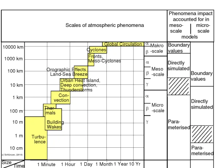
The interactions between urban areas and the atmosphere above imply various scales.Orlanski
(1975) gives a rational subdivision of scales for atmospheric processes:
• synoptic scale (scale of largest cyclones, distance larger than 2000 km)
• mesoscale (between synoptic scale and larger than microscale, from 2000 km to 200 km
and from 200 km to 2 km)
• microscale (near-ground atmospheric phenomena, distance less than 2 km). More
re-cently, microscale includes smaller scales, such as: building scale (less than 100 m), building component scale (less than 10 m) even building material scale.
Scale dependent parameterizations are needed to include the influences of built-up areas on meteorological fields in atmospheric models. In order to study to impact of an urban area on its surroundings (scale varying from 10 to 100 km) mesoscale modeling is used, where the
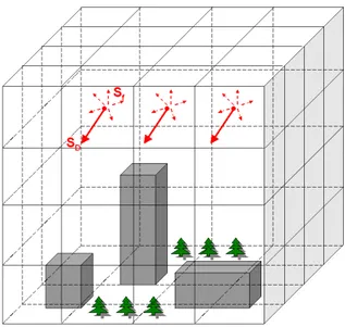
influence of obstacles is parameterized. In order to study the phenomena occurring within the urban canopy (scale varying from 100 m to 2 km) obstacle resolving microscale models are used, where the obstacles are explicitly included in the mesh. Nevertheless, while characteristic scales of phenomena resulting from single obstacles are relatively small (∼ 100 m, ∼ minutes) and can be resolved, in reality there are always multiple obstacles as, for example in urban areas; many buildings, in a wind turbine park; many turbines, or in a forest; many trees. In these cases, hardly all obstacles can be resolved with sufficient detail, and their impacts need to be parameterized (Schlünzen et al., 2011). To additionally calculate the interaction of canopy layer processes and the air above, a coupling between mesoscale and microscale models can be used. Based onOrlanski(1975) and Randerson(1976), Schlünzen et al.(2011) (Fig. 1.1) summarize the spatial scales of phenomena that can be directly simulated in a mesoscale model and microscale model and that have to be parameterized in a model or to be considered via the boundary values. The boundary layer over an urban area is of particular interest as it is in this layer of the atmosphere that the majority of observations in urban areas are made (Oke,1987;
Stull,1988). It is therefore important to know what these observations represent. As air flows from one surface to another an internal boundary layer forms. The internal boundary layer is influenced by the new surface and deepens with fetch. The internal boundary layer formed over urban areas is the urban boundary layer (UBL) (Oke et al., 1999;Stull, 1988). The buildings introduce a large amount of vertical surfaces, high roughness elements, artificial materials, and impervious surfaces (such as buildings and pavements that are made of dark colors absorb the heat which causes the temperature of the surface and surrounding air to increase). The most well-known consequences are the UHI, the generation of local flows between the city centre and its outskirts and between the various city districts, and the "urban plume" downwind of a city. In calm or low wind condition, the warmer air in the city core rises, pulling air near the surface radically inward and a radially outward return flow develop aloft. This air circulation forms the "urban dome"(a dome of heated air above the cities due to pressure differences between warmer temperatures in the city and cooler temperatures in the surrounding rural areas). The
1.2. Urban physics 7
Figure 1.1: Spatial and temporal scales of atmospheric phenomena and how these phenomena are treated in Reynolds-Averaged Navier-Stokes (RANS) mesoscale or obstacle resolving mi-cro scale models (right columns). Dashed areas in the right columns indicate the currently used RANS model resolutions and the resulting possibly resolvable minimum phenomena sizes. FromSchlünzen et al.(2011).
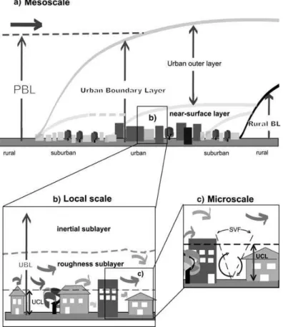
UBL structure and its various sub-layers are depicted in Figure1.2.
Figure 1.2: Schematics of the urban boundary-layer structure indicating the various (sub)layers and their names. a) PBL: planetary boundary layer; in b) UCL: urban canopy layer; in c) SVF: sky view factor. FromRotach et al.(2005); modified afterOke(1987).
1.2.2
Urban energy balance
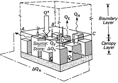
Knowledge of the surface energy balance is essential to understand urban climate and boundary layer processes (Oke, 1987). Oke (1987) defines the energy balance for a building and air volume containing the net radiation Q∗ (W m−2), the sensible heat flux QH (W m−2), the latent heat flux QE (W m−2), storage ∆QS (W m−2), the advective flux∆QA (W m−2), and the anthropogenic heat flux QF (W m−2) as illustrated in Figure1.3, with the following equilibrium
1.2. Urban physics 9
relationship:
Q∗+ QF = QH+ QE+∆QS+∆QA, (1.1) where Q∗ (W m−2) is the net radiation flux through the top of the volume, QF (W m−2) is the anthropogenic heat flux release within the volume, QH (W m−2) and QE (W m−2) refer to convection of sensible heat flux and latent heat flux respectively through the top of the volume. The terms∆QS (W m−2) and∆QA (W m−2) are storage of heat in the ground and the build-ings and advective heat transfer within the volume. Note that here the terms "convection"and "advection"refer to vertical turbulent transfer and mean horizontal transfer, respectively.
For dry surfaces, the energy balance in equation (1.1) is simplified by neglecting QE, and if the sites are horizontally homogeneous,∆QA can be also ignored. Therefore, surface temper-ature results from the balance of energy exchanges at the surface given the incoming radiative forcing, the local ambient air temperature, and the surface radiative properties.
Figure 1.3: Schematics of the urban energy balance in an urban building-air volume. From
Oke(1987). The base of the averaging volume is determined as the level across which there is negligible energy transfer on time scales of less than a day. With: Q∗ (W m−2) is the net radiation; QH (W m−2) the sensible heat flux; QE (W m−2) the latent heat flux;∆QS (W m−2) storage;∆QA (W m−2) the advective flux; and QF (W m−2) the anthropogenic heat flux.
1.2.2.a Radiative balance Q∗
The net radiative flux at a surface reads:
Q∗= S↓− S↑+ L↓− L↑, (1.2)
where S↓ (W m−2) and S↑ (W m−2) are respectively the incoming and outgoing short-wave radiative fluxes, L↓ and L↑ are respectively incoming and outgoing long-wave radiative flux (W m−2).
Incoming short-wave radiation can be decomposed into its direct and diffuse component, and for both short- and long-wave radiation we can distinguish the contributions coming from the atmosphere above and from the urban environment:
S↓= SD+ Sf+ Se, (1.3)
L↓= La+ Le, (1.4)
where SD(W m−2) is the direct solar flux, Sf (W m−2) the solar flux diffused by the atmosphere above, Se (W m−2) the flux diffused by the environment (i.e. from multi-reflection on the surfaces). La(W m−2) and Le(W m−2) are the long-wave radiation flux from the sky and from the multi-reflection on the other surfaces.
Outgoing solar radiation expresses by the albedo (usually writtenα, a dimensionless quan-tity) which is the fraction of solar radiation reflected by a surface. Albedo determines how much solar energy, a particular substance reflects. Hence, S↑reads:
S↑=α(SD+ Sf+ Se). (1.5)
Outgoing long-wave radiation is decomposed into an emitted and reflected part. It is a func-tion of surface temperature Ts f c (K) and surface emissivity (usually writtenε, a dimensionless quantity). Emissivity of a particular material is the fraction of energy that would be radiated by a black body at the same temperature. For a black bodyε would be equal 1, while for any real objectε < 1. Thus, L↑reads:
1.2. Urban physics 11
whereσ is the Stefan-Boltzmann constant (5.66703 × 10⁻⁸W m−2K−4).
1.2.2.b Anthropogenic heat flux QF
Anthropogenic heat flux is generated by humans and human activity, whilst it has a small in-fluence on rural temperatures, it becomes more significant in dense urban areas (Washington,
1972). The American Meteorological Society (AMS) defines it as: “Heat released to the at-mosphere as a result of human activities, often involving combustion of fuels. Sources include industrial plants, space heating and cooling, human metabolism, and vehicle exhausts. In cities this source typically contributes 15∼ 50 W m−2to the local heat balance, and several hundred
W m−2in the center of large cities in cold climates and industrial areas.”
Anthropogenic heat flux is one contributor to urban heat islands. Although it is usually smaller compared to other fluxes, its influence is observable (Pigeon et al., 2007). Anthro-pogenic heat generation can be estimated by adding all the energy used for heating and cooling, running appliances, transportation, industrial processes, plus that directly emitted by human metabolism.
1.2.2.c Sensible heat flux QH
Surface sensible heat flux is the energy exchanged between a surface and the air in the presence of a surface-air thermal gradient. Modeling the sensible heat flux contributes to determine both stratification effects on turbulent transport, and to estimate the surface temperature. The sensible heat flux QH can be parameterized as:
QH = hf(Ta− Ts f c), (1.7)
in which hf (W m−2K−1) is the heat transfer coefficient and Ta(K) the air temperature.
We give a detailed comparison between different approaches to model the heat transfer coefficient in Chapter 3.
1.2.2.d Storage heat flux∆QS
The storage heat flux is a significant component of the energy balance (Grimmond and Oke,
1999b). Knowledge of the storage heat flux term is required in a variety of applications, for example to model evapotranspiration, sensible heat flux, boundary layer growth, etc. Further-more, the thermal inertia provided by this storage term is often regarded as a key process in urban heat islands. It accounts for 17% to 58% of the daytime net radiation, and is greater at the more urbanized sites (downtown and light industrial) (Grimmond and Oke, 1999b). Con-sidered at the hourly timescale∆QSis variable. However,∆QS is difficult to measure or model because of the complex three-dimensional structure of the urban surface and the diversity of materials. It is often determined as the residual of the surface energy balance equation ( Grim-mond and Oke,1999b).
Camuffo and Bernardi(1982),Grimmond and Oke(1999b) suggest a hysteresis-type equa-tion to characterize the storage heat flux as a linear funcequa-tion of Q∗and of the temporal variation of Q∗:
∆QS= a1Q∗+ a2∂ Q∗
∂t + a3, (1.8)
where t (s) is time. The parameter a1 describes the overall strength of the dependence of the
storage heat flux on net radiation. The parameter a2is the coefficient of retardation of∆QSwith respect to Q∗. The parameter a3is an intercept term that indicates the relative time when∆QS and Q∗turn negative. Parameters a1, a2and a3can be calculated through regression for hourly
averaged data.
1.3
Objectives and structure of the thesis
This work aims to contribute to study the detailed energy exchanges between buildings and the urban atmosphere (the distribution of surface temperatures). It involves developing a model coupling thermal transfers involving the buildings and a Computational Fluid Dynamics (CFD) modeling of the atmosphere in an urban area. The numerical model used is the atmospheric
1.3. Objectives and structure of the thesis 13
module of the three-dimensional open source CFD code Code_Saturne developed by EDF and CEREA. In previous work, a microscale three-dimensional atmospheric radiative scheme has been implemented in the code to model the energy balance for complex geometries (Milliez,
2006). The surface temperature is modeled with a simple approach, the force-restore method. The new scheme has been validated with simple cases found in the literature (Milliez,2006).
Four objectives of this research are as follows:
• The first objective of the thesis is to improve the heat transfer model in buildings, by
testing two modeling approaches: the force-restore model and a one dimensional con-duction scheme. For both approaches, the aim is to perform sensitivity studies to thermal parameters and material properties and in particular to internal building temperature.
• The second objective is to compare with another 3D radiative model which uses the
geometric view factor approach: the SOLENE model (Miguet and Groleau, 2002). The comparison are made for the short-wave direct and diffused fluxes, long-wave incoming fluxes and surface temperatures.
• The third objective is to study the full radiative-convective coupling. In most models
tak-ing into account the radiation in built-up environment (integrative or three-dimensional models), the airflow, required for calculating the convective flux, is parameterized and rarely fully modeled. The radiative and thermal models implemented in the CFD code
Code_Saturne has the advantage of being coupled with the dynamic module, in particular
through the use of a common mesh.
However, in previous studies (Milliez, 2006), the radiative-dynamical interaction has been discussed in a simple way, using a constant pre-calculated and thus decoupled flow field. The full radiative-dynamical coupling is nevertheless already implemented, it needs to be studied in detail in this thesis, including the thermal impact on airflow and on surface temperatures of taking into account a three-dimensional flow field for the computation of convective fluxes. Such a detailed study (which may be computationally
expensive) may provide a better understanding of the phenomena at microscale.
• The last objective includes the validation of our approach with field measurements on an
idealized urban environment as well as on a real city district. This requires a detailed analysis of the available data sets in order to identify the surface properties, the input and meteorological data (radiative fluxes and wind) as well as mesh generation of very complex geometries.
In Chapter 2, I first present some basic CFD aspects and urban energy models, then de-scribe our dynamical coupled model. Chapter 3 presents a validation of the radiative-dynamical model with observations (MUST field experiment) and compares three schemes of increasing complexity for predicting convective flux (published paper). In Chapter 4, I compare our radiative model with the SOLENE model. Chapter 5 consists a numerical investigation on the thermal impact on a low wind speed airflow within an idealized built-up area (submitted paper). In Chapter 6, I perform numerical simulation of a real urban area case (a district of Toulouse, CAPITOUL case) including data analysis, complex mesh generation and simulation results. Chapter 7 highlights the main conclusions and provides perspectives for future work.
C
HAPTER
2
Model design
Contents
2.1 General CFD modeling approach for the urban environment . . . . 15
2.1.1 Best practice guidelines . . . 18
2.1.2 Mesh issues . . . 27
2.2 Review of some Urban Energy Balance Models . . . . 32
2.2.1 Urban Energy Balance Modeling. . . 32
2.2.2 International Urban Energy Balance Models Comparison . . . 35
2.3 A new coupled radiative-dynamic 3D scheme in Code_Saturne for modeling urban areas . . . . 38
2.3.1 Presentation of the atmospheric module in Code_Saturne . . . 39
2.3.2 3D Atmospheric Radiative model . . . 42
2.3.3 Surface temperature models . . . 47
2.3.4 Convection model . . . 50
2.1
General CFD modeling approach for the urban
environ-ment
In the past decades, Computational Fluid Dynamics has been intensively used to evaluate the indoor environment of buildings and heat and mass transfer between the indoor environment
and the building envelope (Loomans et al.,2008). It has also been used in research on wind flow and the related processes in the outdoor environment around buildings, including pedestrian wind comfort (Blocken, 2009), wind-driven rain on building frontage (Briggen et al., 2009), pollutant dispersion (Hanna et al., 2006), exterior surface heat transfer (Blocken et al., 2009), natural ventilation and wind load of buildings (Cook et al.,2003). For both indoor and outdoor environment studies, the advances in computing performance and the development of efficient and powerful grid generation techniques and numerical solvers have led to the present situation in which CFD can technically be applied for study cases involving complex geometries and complex flow fields.
Numerical CFD modeling offers considerable advantages because it allows investigation where experimentation is not possible. It can provide a large amount of detail about a flow in the whole calculation domain, under varied conditions and without similarity constraints. The main limitations are the requirement of systematic and CFD solution verification and validation studies. The Navier-Stokes equations are commonly used to model the flow in the atmospheric boundary layer (ABL) and the nature of the flow in an urban area, consisting of an arbitrary ag-gregation of buildings, is dominated by unsteady turbulent structures. Unfortunately, turbulent flow is one of the unsolved problems of classical physics. Despite many years of intensive re-search, a complete understanding of turbulent flow has not yet been attained (Davidson,2004). Several methods exist for predicting turbulent flows with CFD. Three most popular approaches are: Direct Numerical Simulation (DNS), Large Eddy Simulation (LES) and Reynolds-Averaged Navier-Stokes (RANS) simulation. The three approaches including the choice for our simulations have already been introduced in a previous work (seeMilliez(2006) Chapter 2). Here, we just briefly present the advantages and weaknesses of each simulation approach.
Direct Numerical Simulation (DNS) DNS solves the exact Navier-Stokes equations by re-solving all the scales of motion from the energetic large scales to the dissipative small scales, without any modeling. In consequence, DNS is expected to provide accurate predictions of
2.1. General CFD modeling approach for the urban environment 17
the flow (Moin and Mahesh, 1998). However, the associated computational cost is extremely expensive in the case of urban flow problems. Indeed, the number of grid points required to simulate a three-dimensional turbulent flow in DNS is proportional to Re9L/4, where ReL is the Reynolds number based on the integral scale of the flow. Because the time step is related to the grid size, the total computational cost for DNS actually increases as Re3L. This rapid increase with ReL prohibits the application of DNS to high Reynolds number flows, such as the ones in the ABL. Despite of all progress in terms of computational power, DNS is still restricted to flows with low Reynolds numbers in relatively simple obstacles in urban areas because of the very large range of scales that have to be resolved (Coceal et al.,2007) .
Large Eddy Simulation (LES) The basic idea of LES is to solve "filtered" Navier-Stokes equations, therefore to resolve only the large-scale motions in a turbulent flow and model the small-scale (unresolved) motions. The latter scales of motion are expected to be more universal and, hence, easier to model. Compared to DNS, LES is not an exact solution but is less com-putationally demanding. However, the application of LES to wall-bounded flows, particularly at high Reynolds numbers, is severely restricted owing to the grid resolution requirements for LES to resolve the viscous small-scale motions near the wall. Chapman(1979) estimated that the number of grid points needed for LES to resolve these near-wall small-scale motions is approximately proportional to Re1L.8. Several LES studies have been applied to study ABL flow and dispersion in urban areas (Kanda et al., 2004;Xie et al., 2008;Santiago et al., 2010). In spite of the fact that LES computations are feasible and more accurate than Reynolds-Averaged Navier-Stokes simulation (see next paragrah) but they are still very expensive.
Reynolds-Averaged Navier-Stokes simulation (RANS) As the name implies, the RANS approach solves the "averaged" Navier-Stokes equations. In this approach, only the ensemble averaged flow properties are resolved with all other scales of eddies being modeled. The tur-bulent stresses required for the closure of the Reynolds-averaged momentum equation, known as the Reynolds stresses, represent the mean momentum fluxes induced by turbulence. The
classical approach to model this term is to adopt the eddy viscosity concept originally proposed byBoussinesq(1877), which assumes a linear constitutive relationship between the turbulent stresses and the mean strain-rate tensors.
As additional equations, several types of turbulence models allow to obtain an estimate for the Reynolds stresses in the RANS equations: Mixing length model (Prandtl, 1925), k−ε turbulence models (standard, renormalization group (RNG), realizable) (Launder and Spald-ing,1974;Yakhot et al.,1992), k−ω turbulence models (Kato and Launder,1993), Algebraic stress models (Baldwin and Lomax,1978) and Reynolds stress models (Launder et al., 1975). The computational cost of RANS is independent of the Reynolds number, except for wall-bounded flows where the number of grid points required in the near-wall region is proportional to ln(ReL) (Pope, 2000). Although RANS is less accurate, because of its computational effi-ciency, RANS is the most commonly used CFD methodology for the simulation of turbulent flows encountered in industrial and engineering applications. Note that there is no turbulence model that is universally valid. In our simulations, the turbulence is parameterized by the well known standard k−ε closure .
2.1.1
Best practice guidelines
The accuracy of CFD is an important matter of concern. Care is required in the geometrical implementation of the model, in grid generation and in selecting proper solution set-up and parameters. Since a large number of choices needs to be made by the user in CFD simulations, some guidelines on industrial applications have been published in order to clarify the method for validation and verification of CFD results (e.g. ERCOFTAC (European Research Commu-nity on Fluids, Turbulence And Combustion) organizations’ guidelines (Casey and Winterg-erste, 2000)). In 2007, European Cooperation in Science and Technology (COST action 732 research group) (Franke et al.,2007) compiled a set of specific recommendations for the use of CFD in wind engineering from a detailed review of the literature. In2008, a Working Group in the Architectural Institute of Japan (AIJ) (Tominaga et al.,2008), similar to COST 732,
con-2.1. General CFD modeling approach for the urban environment 19
ducted extensive best practice advice for CFD prediction fo the pedestrian wind environment around buildings. These documents primarily focused on steady RANS simulations. Here, we briefly present some guidelines for CFD in urban aerodynamics which are mainly based on COST (Franke et al.,2007) and AIJ (Tominaga et al.,2008) recommendations.
2.1.1.a Error in CFD Simulations
In typical CFD simulations, different kinds of errors can have a very large impact on the results. Here we classify some sources of errors:
Physical modeling errors Physical modeling errors are due to uncertainties in the formu-lation and to deliberate simplifications of the model: for instance, the RANS equations in combination with a given turbulence model, the eddy viscosity model or Boussinesq hypothe-sis, use of specific constants in the k−ε model, use of wall functions, modeling of the surface roughness, simplifications of the geometry, etc. In general, physical modeling errors can be examined by performing validation studies that focus on certain phenomena (e.g. turbulent boundary layers).
Computer round-off errors Computer round-off errors develop with the representation of floating point numbers and the accuracy at which numbers are stored. With advanced computer resources, numbers are typically stored with 16, 32, or 64 bits. Computer round-off errors are not considered significant when compared with other errors. If they are suspected to be significant, one can perform a test by running the code at a higher precision. For simple flows, single precision runs (32 bit arithmetic) are usually adequate for convergence. In some more difficult cases, where there may be extremes of scales in the problem or very fine meshes, it can be required to use double precision (64 bit arithmetic). This will require more memory, but may not add a huge overhead on computational time, depending on the nature of the hardware being used. The computer numbering format in the CFD code Code_Saturne used in our simulations is double precision.
Iteration-convergence error This error is introduced because the iterative procedure to reach the steady state solution has to be stopped at a certain moment in time. The default values for convergence in most commercial codes are not strict because code vendors want to stress calculation efficiency. Therefore, stricter convergence criteria are required to check that there is no change in the solution. COST 732 (Franke et al.,2007) suggests that scaled residuals should drop by at least 4 orders of magnitude. AIJ (Tominaga et al., 2008) points that the suitable convergence values are largely dependent on flow configuration and boundary conditions, so it is better to check the solution directly using different convergence criteria. In our simulations with Code_Saturne, we keep a standard residual value (10−9) and check the convergence of the solution with monitoring points.
Spatial and temporal discretization errors These errors are generated from representing the governing equations on a mesh that represents a discretized computational domain. For unsteady calculations also time discretization causes discretization errors. ERCOFTAC report (Casey and Wintergerste,2000) indicates that the spatial and temporal discretization are prob-ably the most crucial source of numerical errors. The COST 732 report (Franke et al., 2007) advises that grid sensitivity analysis is a minimum requirement in a CFD simulation. In Section (2.1.2), we discuss in more detail the issues relative to the computational grid. To assess the in-fluence of the time step on the results, a systematic reduction or increase of the time step should be made, and the simulation repeated. We investigate this point with the MUST experiment in Chapter 3. In advection dominated problems, the time step∆t (s) should satisfy the following
criteria:
∆t= CFL∆xmin/Umax (2.1)
where∆xmin (m) is the minimum grid width, Umax (m s−1) is the maximum velocity and CFL is the Courant-Friedrichs-Lewy number (Courant et al., 1967). Choosing the minimum grid spacing and the maximum velocity makes this estimate conservative. The generally suggested criteria that CFL< 1.
2.1. General CFD modeling approach for the urban environment 21
used within the model, the influence of the unwise choice of these parameters can also lead to error on the results if the choice is inadequate (see the sensitivity study in Chapter 3).
Generally, many errors are made by CFD users because of lack of knowledge. As a result, simulation results can only be trusted or used if they have been performed on a mesh obtained by grid-sensitivity analysis, performed taking into account the proper guidelines that have been published in literature and carefully validated. Validation means systematically comparing CFD results with experiments to assess the performance of the physical modeling choices.
2.1.1.b Choice of the computational domain
The size of the entire computational domain in the vertical, lateral and flow directions depends on the area that shall be represented and on the boundary conditions that will be used. For urban areas with multiple buildings, both COST 732 (Franke et al., 2007) and AIJ (Tominaga et al.,
2008) reports suggest that the top boundary should be set 5Hmax or above the tallest building with height Hmax (Fig. 2.1). The reason is that the large distances given above the obstacles are necessary to prevent an artificial acceleration of the flow over the buildings. AfterFranke
Figure 2.1: Recommended computational domain size where Hmax refers the maximum height of the building, adapted afterFranke et al.(2007) andTominaga et al.(2008).
et al.(2007), the lateral boundaries should be at a distance of 5Hmax from the obstacles. Same distance should be set between the inlet boundary and the first building which allows for a fully developed flow (Fig. 2.1). The outflow boundary should be positioned at least 15Hmax behind the last building to allow for flow re-development behind the wake region (Fig. 2.1). Similar requirements for the lateral and the inlet boundaries were suggested byTominaga et al.(2008). However, they report that there is a possibility of unrealistic results if the computational region is expanded without representation of surroundings, then the recommended outflow boundaries is at least 10Hmax.
2.1.1.c Initial and boundary conditions
Incorrect or inappropriate specification of initial or boundary conditions is a very common cause of errors. They may lead to the solution of the wrong problem as well as convergence difficulties.
Initial conditions Initial data and inflow data are very often chosen the same. This is a good starting point for most models. Initializing with the larger-scale field which is expected to be close to the final solution will reduce the computational efforts needed to reach stationary so-lutions. However, if these initial data are not close to the real initial conditions (e.g. wrong wind direction) then an accurate solution can not be expected. Since initial data are not known perfectly, but include uncertainties that result from lack of measurement or measurement in-accuracy, the initial input values are never perfectly known. Therefore Franke et al. (2007) advise to keep initial data uncertainty as little as possible and to keep in mind that the initial data influence the model results in unsteady simulations.
Inlet boundary conditions The proper choice of boundary conditions is very important. Since they represent the influence of the larger-scale surroundings and they determine to a large extent the solution inside the computational domain. At the inlet boundary, the mean velocity profile is often obtained from the academic logarithmic profile modeling the flow over
2.1. General CFD modeling approach for the urban environment 23
the upwind terrain via the roughness length z0(m), or from the profiles of the wind tunnel
sim-ulations. In simulation of field experiments, available information from nearby meteorological stations is used to determine the wind speed Ure f (ms−1) at a reference height zre f (m) (Stull,
1988).
In the case the vertical distribution of turbulent energy k(z) (m2 s−2) is not available in the
data set,Franke et al.(2007) assuming a constant friction velocity in ABL, suggest:
k(z) = U ∗2
ABL √
Cµ, (2.2)
and the dissipation rateε(z) can be expressed as:
ε(z) = U ∗3
ABL
κ(z + z0)
, (2.3)
where UABL∗ (m s−1) represents the atmospheric boundary layer friction velocity, Cµ is a con-stant coefficient (= 0.09),κ is the von Karman constant (= 0.4).
Nevertheless,Tominaga et al.(2008) point out that, in their recommendations,Franke et al.
(2007) assume that the height of the computational domain is much lower than the atmospheric boundary layer height, since the assumption of a constant friction velocity is only valid in the lower part of the atmospheric boundary layer - surface boundary layer (Stull,1988). Therefore, AIJ (Tominaga et al., 2008) proposed the following estimation equation between the vertical profile of turbulent intensity I(z) and turbulent energy k(z):
k(z) = I(z)2U(z)2, (2.4)
with
I(z) = 0.1( z zG
)−β−0.05, (2.5)
where U(z) is the vertical velocity (ms−1), zG (m) is the boundary layer height and β is the power-law exponent. Both zGandβ are determined by terrain category, and
ε(z) = C1µ/2k(z)Ure f zre f β
( z zre f
Top boundary conditions AIJ (Tominaga et al., 2008) report that if the computational do-main is large enough (Fig. 2.1), the boundary conditions for lateral and top boundaries do not have significant influences on the calculated results around the target buildings. However, the COST 732Franke et al.(2007) report stresses the importance of the choice of the top boundary condition and lateral boundary conditions. If symmetry boundary conditions are applied to the top boundary, these might enforce a parallel flow, by forcing the velocity component normal to the boundary to vanish. Furthermore, prescribing zero normal derivatives for all other flow variables may lead to a change from the inflow boundary profiles (which can have a non zero gradient at the height of the top of the domain). On the other hand, if the top boundary is handled as an outflow boundary, it can allow a normal velocity component at this boundary. In order to prevent a horizontal change from the inflow profiles, it is recommended to prescribe a constant shear stress at the top. The latter option is taken in our simulations (see Chapter 5 and 6).
Lateral boundary conditions In the CFD codes, when the approach flow direction is parallel to the lateral boundaries, symmetry boundary conditions are frequently used at lateral bound-aries. We use this option in an idealized case simulation (see Chapter 5). Franke et al.(2007) state that symmetry boundary conditions enforce a parallel flow by requiring a vanishing nor-mal velocity component at the boundary. Therefore, the boundary should be positioned far enough from the built-up area of interest in order not to lead to an artificial acceleration of the flow near the lateral boundaries (Fig. 2.1). In the case where different wind directions are to be simulated with the same computational domain, then the lateral boundaries become inflow or outflow boundaries. They are cases we present in Chapter 3 and 6.
Outlet boundary conditions At the boundary behind the obstacles (where all or most of the fluid leaves the computational domain), open boundary conditions are mostly used in CFD sim-ulations. The open boundary conditions are either outflow or constant static pressure boundary conditions. We apply the outflow boundary conditions in our simulations. With an outflow
2.1. General CFD modeling approach for the urban environment 25
boundary condition, the derivatives of all flow variables are forced to zero, corresponding to a fully developed flow. Franke et al. (2007) indicate that this boundary should be ideally far enough from the last building in order not to have any fluid re-entering into the computational domain. This also applies when using a constant static pressure at the outflow boundary, with the derivatives of all other flow variables forced to vanish. We note that imposed pressure at outlet is used in Code_Saturne.
Wall boundary conditions At solid walls, the no-slip boundary condition is used for the velocities. Franke et al.(2007) mention two different approaches to resolve the shear stress at smooth walls. The first one is the low-Reynolds number approach which resolves the viscous sublayer and computes the wall shear stress from the local velocity gradient normal to the wall. The equations for the turbulence quantities contain damping functions to reduce the influence of turbulence in this region dominated by molecular viscosity. The low-Reynolds number approach requires a very fine mesh resolution in the wall-normal direction. The first computational node should be positioned at a dimensionless wall distance z+given by:
z+= zuτ/ν≈ 1, (2.7)
where z (m) is the distance normal to the wall,ν (m2s−1) is the the kinematic viscosity and uτ (m s−1) is the shear velocity, computed from the time averaged wall shear stressτw(N m−2):
uτ = (τw/ρ)1/2, (2.8)
withρ (kg m−3) the density.
To reduce the number of grid points in the wall-normal direction and therefore the com-putational costs, another approach called wall functions is applied as an alternative approach to compute the wall shear stress. With the wall function approach, the wall shear stress is computed assuming a logarithmic velocity profile between the wall and the first computational node in the wall-normal direction. For the logarithmic profile to be valid, the first computational node should be placed at a dimensionless wall distance of z+ between 30 and 500 for smooth
walls. Also, for wall function modeling the turbulence quantities have to be modified at the first computational node. They are usually calculated assuming an equilibrium boundary layer, consistent with the logarithmic velocity profile. In spite of invalid in regions of flow separation, of reattachment and of strong pressure gradients and also unpredictable of the transition from laminar to turbulent boundary, the effect of wall functions on the solution away from the wall is however regarded as small in the built environment.
Furthermore, the wall function approach is also used for rough walls. Blocken et al.(2007) state different wall functions and demonstrate the importance of four basic requirements for CFD simulation of ABL flow with sand-grain wall functions. The four requirements are:
• a high mesh resolution in the vertical direction near the bottom of the computational
domain,
• the horizontal homogeneity of ABL flow in the upstream and downstream region of the
domain,
• a distance yP (m) from the center point P of the wall-adjacent cell to the wall (bottom of the domain) that is larger than the physical roughness height kS (m) of the terrain (yP> kS),
• the relationship between the equivalent roughness height kSand the corresponding aero-dynamic roughness length z0(m).
In order to deal with the problem of the impossibility of simultaneously satisfying all four requirements in the kstype wall functions for fully rough surfaces (i.e. standard wall functions modified for roughness based on experiments with sand-grain roughness),Blocken et al.(2007) consider that the best solution is to violate the third requirement yP> kSand advise to assess the extent of horizontal inhomogeneity by a simulation in an empty computational domain prior to the simulation domain with obstacles. A roughness wall function is used in our simulations, and is presented in Section2.3.4. We also apply the similar consideration to the thermal boundary layer for heated walls.
2.1. General CFD modeling approach for the urban environment 27
2.1.1.d Algorithmic Considerations
In order to be numerically solved, the basic equations have to be discretized and transformed into algebraic equations. For time-dependent problems, second-order methods should also be chosen for the approximation of the time derivatives. Higher order advection differenc-ing schemes can lead to to numerical oscillations that may cause poor convergence, or have quantities to overshoot. Running with first order upwind schemes may help to overcome this. However, it should be recalled that the spatial gradients of the transported quantities tend to become diffusive due to a large numerical viscosity of the upwind scheme. Both COST 732 (Franke et al., 2007) and AIJ (Tominaga et al., 2008) reports do not recommend the use of first-order methods like upwind scheme except in initial iterations.
In this research, I first performed the simulations which are presented in Chapter 3 with a center scheme. However, when the thermal effects are taken into account in a low wind speed case (Chapter 5), using a center scheme happens to creat numerical instabilities, especially in the inflow region and an upwind scheme is used. We adapt the same choice for the simulation in Chapter 6.
2.1.2
Mesh issues
The discrete spatial domain (either for Finite-Difference, Finite-Volume or Finite-Element methods) is known as the grid or mesh. Mesh generation is often considered as the most important and most time consuming part of CFD simulations. The quality of the mesh plays a direct role in the quality of the simulations, regardless of the flow solver used. Additionally, the solver will be more robust and efficient when using a well constructed mesh.
2.1.2.a Mesh classification
As CFD has developed, better algorithms and more computational power have become avail-able, resulting in a diversification in solver techniques. One direct result of this development has been the expansion of available mesh elements and mesh connectivity (how cells are
con-nected to one another). The elements in a mesh can be classified in various ways. Based on the connectivity of the mesh, they can be classified: structured or unstructured. Structured grid generators are most commonly used when strict elemental alignment is mandated by the analysis code or is necessary to capture physical phenomenon. Unstructured mesh generation, on the other hand, relaxes the node valence requirement, allowing any number of elements to meet at a single node. Code_Saturne can work with both a structured grid and an unstructured mesh. Another mesh classification is based on the dimension and type of the elements. Com-mon elements in 2D are triangles or rectangles, and comCom-mon elements in 3D are tetrahedral or hexahedral. Here we briefly describe the types of meshes which are commonly used.
Hexahedral meshes Hexahedral meshes (either structured or unstructured grids) take their name from the fact that the mesh is characterized by a polyhedron with six faces. Although the element topology is fixed, the mesh can be shaped to be body fitted through stretching and twisting of the grid. Hexahedral meshes have the advantage of allowing a high degree of control. Indeed, hexahedral grids, which are very efficient at filling space, support a high degree of skewness and stretching before the solution is significantly affected. Also, the mesh can be flow-aligned, thereby yielding to greater accuracy of the solver. Hexahedral mesh flow solvers typically require lower amount of memory for a given mesh size and execute faster because they are optimized for the structured layout of the mesh. Lastly, post processing of the results on a hexahedral block mesh is typically a much easier task. Because the logical mesh planes make excellent reference points for examining the flow field and plotting the results.
Compared to tetrahedral meshes (see next paragraph), for the same cell count, hexahedral meshes will give more accurate solutions, especially if the grid lines are aligned with the flow. The major drawback of hexahedral meshes is the time and expertise required to lay out an optimal block structure for an entire model. Some complex geometries (see the CAPITOUL mesh in Chapter 6) are very hard even impossible to mesh with hexahedral block topologies. In these areas, the user is forced to stretch or twist the elements to a degree which drastically affects solver accuracy and performance. With the present computational power, mesh
genera-2.1. General CFD modeling approach for the urban environment 29
tion times are usually measured in hours if not days. We use this type of the mesh in the simple building geometry case (see Chapter 3 MUST mesh).
Tetrahedral meshes Tetrahedral meshes (always unstructured grids) are characterized by irregular connectivity which is not readily expressed as a three dimensional array in computer memory, but use an arbitrary collection of elements to fill the domain. Tetrahedral meshes can be stretched and twisted to fit the domain. These methods have the ability to be automated to a large degree. Given a good Computer-Aided Design (CAD, hereafter) model, a good mesher can automatically place triangles on the surfaces and tetrahedral in the volume with very little input from the user. The advantage of tetrahedral mesh methods is that they are very automated and, therefore, require little user time or effort. And we do not need to worry about laying out block structure or connections. Mesh generation times are usually measured in minutes or hours.
The major drawback of tetrahedral meshes is the lack of user control when laying out the mesh. Typically any user involvement is limited to the boundaries of the mesh with the mesher automatically filling the interior. Triangle and tetrahedral elements have the problem that they do not stretch or twist well, therefore, the mesh is limited to being largely isotropic, i.e. all the elements have roughly the same size and shape. This is a major problem when trying to refine the mesh in a local area, often the entire mesh must be made much finer in order to get the point densities required locally. Another drawback of the methods is their reliance on good CAD data. Most meshing failures are due to some (possibly minuscule) error in the CAD model. Tetrahedral flow solvers typically require more memory and have longer execution times than structured hexahedral mesh solvers on a similar geometry. Post processing the solution on a tetrahedral mesh requires powerful tools for interpolating the results onto planes and surfaces of rotation for easier viewing. Since Code_Saturne accepts meshes with any type of cell and any type of grid structure and we have an available CAD data, we use this type of the mesh in CAPITOUL studies (see the CAPITOUL mesh in Chapter 6).
Hybrid meshes A hybrid mesh is a mesh that contains hexahedral portions and tetrahedral portions. Hybrid meshes are designed to take advantage of the positive aspects of both hexa-hedral and tetrahexa-hedral meshes. They use some form of hexahexa-hedral cells in local regions while using tetrahedral cells in the bulk of the domain. Hybrid meshes contain hexahedral, tetrahe-dral, prismatic, and pyramid elements in 3D and triangles and quadrilaterals in 2D. The various elements are used according to their strengths and weaknesses. Hexahedral elements are ex-cellent near solid boundaries (where the gradients are high) and afford the user a high degree of control, but are time consuming to generate. Prismatic elements (usually triangles extruded into wedges) are useful for resolving near wall gradients, but suffer from the fact that they are difficult to cluster in the lateral direction due to the underlying triangular structure. In almost all cases, tetrahedral elements are used to fill the remaining volume. Pyramid elements are used to transition from hexahedral elements to tetrahedral elements. Many codes try to automate the generation of prismatic meshes by allowing the user to define the surface mesh and then marching off the surface to create the 3D elements. While very useful and effective for smooth shapes, the extrusion process can break down near regions of high curvature or sharp disconti-nuities. The advantage of hybrid mesh methods is to control the shape and distribution of the grid locally, which can yield excellent meshes. The disadvantage is that they can be difficult to use and require user expertise in laying out the various grid locations and properties to get the best results. The generation of the hexahedral portions of the mesh will often fail due to complex geometry or user input errors. While the flow solver will use more resources than a structured hexahedral block code, it should be very similar to an unstructured tetrahedral code. Post processing the flow field solution on a hybrid grid suffers from the same disadvantages as a tetrahedral mesh. The time required for mesh generation is usually measured in hours or days.
2.1. General CFD modeling approach for the urban environment 31
2.1.2.b Choice of the computational mesh
With the Finite Volume, Finite Difference and Finite element methods the computational results depend crucially on the mesh that is used to discretise the computational domain. A high quality mesh should allow capturing the important physical phenomena like shear layers or vortices with sufficient resolution and no large errors introduced.
Geometrical representation of obstacles The level of details required for individual build-ings or obstacles depends on their distance from the central area of interest. Franke et al.(2007) point out that the central area of interest should be reproduced with as much details as possible. This naturally increases the number of cells that are necessary to resolve the details. The avail-able computational resources therefore limit the details which can be reproduced. Nevertheless, the numerical studies do not always require a very high degree of details. In our simulations, buildings will be represented as simple blocks (see Chapter 3, the MUST experiment or with more details in Chapter 6 the CAPITOUL experiment).
Mesh resolution When a global systematic mesh refinement is not possible due to resource limitations, at least a local mesh refinement should be used in the areas of interest. Grid stretch-ing/compression should be small in regions of high gradients to keep the truncation error small. In these regions, bothFranke et al.(2007) andTominaga et al.(2008) advise an expansion ratio of 1.3 or less.Tominaga et al.(2008) suggest that the minimum grid resolution should be set to about 1/10 of the building height scale (about 0.5 to 5.0m) within the region including the
eval-uation points around the target building. Moreover, the evaleval-uation height (1.5 to 5.0m above
ground) should be located at the third or higher grid cell from the ground surface. Franke et al.
(2007) suggest that at least 10 cells should be used per building side and 10 cells per cube root of building volume as an initial choice. It is also recommended that pedestrian wind speeds at 1.5 to 2m height should be calculated at the third or fourth cell above the ground.
The mesh should be generated with consideration of such things as resolution, density, as-pect ratio, stretching, orthogonality, grid singularities, and zonal boundary interfaces. However,
the sensitivity of the results on the mesh resolution should be tested. Franke et al.(2007) and
Tominaga et al. (2008) indicate that the number of fine meshes should be at least 1.5 times
the number of coarse meshes in each dimension, and at least three refined meshes should be tested. Additionally, for the unstructured mesh, it is necessary to ensure that the aspect ratios do not become excessive in regions adjacent to coarse girds or near the surfaces of complex geometries. For improved accuracy, it is recommended to arrange the boundary layer elements (prismatic cells) parallel to the walls or the ground surfaces (Fig. 2). BothFranke et al.(2007) andTominaga et al.(2008) introduce the same technique.
2.2
Review of some Urban Energy Balance Models
2.2.1
Urban Energy Balance Modeling
The behavior of the atmospheric Urban Canopy Layer (UCL) is the result of the interactions between atmospheric structures induced by the urban heterogeneities. One important feature of the UCL is the urban energy balance. The recent years, Surface Energy Balance (SEB) models have evolved rapidly and increased in complexity, with increasing computer power and development of micrometeorological parameterizations.
A large number of models now exist with different assumptions about the important features of the surface and exchange processes that need to be incorporated. They can be classified into five categories, depending on the complexity of the parametrization, each one having its advantages and weaknesses (Masson,2006;Milliez,2006):
• Empirical models: this type of approach makes it possible to use extremely simple
schemes. For instance, the Local-scale Urban Meteoro-logical Parameterization Scheme (LUMPS) (Grimmond and Oke,2002) is a local-scale urban meteorological parameteri-zation scheme capable of predicting the 1D spatial and temporal variability in heat fluxes in urban areas. Their main weakness is that they are based on statistics from field data, therefore they are limited to the range of conditions (land cover, climate, season, etc.)
2.2. Review of some Urban Energy Balance Models 33
encountered in the original studies (Masson,2006).
• Vegetation models without drag terms: this type of approach is based on the
observa-tion that roughness lengths and displacement heights are large over cities. Some refine-ment, depending on how the buildings are spatially organized, can be used to evaluate the roughness lengths. When coupled to an atmospheric model, the first atmospheric level is above the surface scheme, with all the friction located at this level. Grimmond and Oke
(1999a) analyze the nature, sensitivity, and size of aerodynamic parameters obtained us-ing morphometric methods, especially in the context of the physical structure of parts of North American cities.
• Vegetation models with drag terms: these models are derived from forest canopy
parame-terizations. A drag force is directly added in the equations of motions in the atmospheric model, up to the height of the highest buildings. Additional terms in the turbulence equa-tion can also be taken into account. The main disadvantage of drag based schemes is that they imply direct modification of the equations of the atmospheric models to which they are coupled. The Soil Model for Submesoscales, Urbanized Version (SM2-U) (Dupont et al., 2004), includes a one-layer urban-and-vegetation canopy model to integrate the physical processes inside the urban canopy and three soil layers. The physical processes inside the urban canopy, such as heat exchanges, heat storage, radiation trapping, wa-ter inwa-terception, or surface wawa-ter runoff, are integrated in a simple way (e.g. neither separated walls and roads energy budgets nor wind speed parameterization inside the canopy).
• Single layer schemes: in this approach, the exchanges between the surface and the
at-mosphere occur at the top of the canopy. This means that, when this scheme is coupled with an atmospheric model, the first level of the atmospheric model is located above the roof level. This has the advantage of simplicity and transferability. In this approach, the characteristics of the air in the canopy must be parametrized. In general, the logarithmic