HAL Id: hal-01616931
https://hal.archives-ouvertes.fr/hal-01616931
Submitted on 17 Oct 2017
HAL is a multi-disciplinary open access
archive for the deposit and dissemination of
sci-entific research documents, whether they are
pub-lished or not. The documents may come from
teaching and research institutions in France or
abroad, or from public or private research centers.
L’archive ouverte pluridisciplinaire HAL, est
destinée au dépôt et à la diffusion de documents
scientifiques de niveau recherche, publiés ou non,
émanant des établissements d’enseignement et de
recherche français ou étrangers, des laboratoires
publics ou privés.
An Incremental Constituve Law for Damaging
Viscoelastic Materials
Omar Saifouni, Rostand Moutou Pitti, Jean-Francois Destrebecq
To cite this version:
Omar Saifouni, Rostand Moutou Pitti, Jean-Francois Destrebecq. An Incremental Constituve Law
for Damaging Viscoelastic Materials. Tom Proulx. Mechanics of Time-Dependent Materials and
Processes in Conventional and Multifunctional Materials, 3, Springer, pp.241-248, 2011,
978-1-4614-0213-8. �10.1007/978-1-4614-0213-8_35�. �hal-01616931�
AN INCREMENTAL CONSTITUVE LAW FOR DAMAGING VISCOELASTIC
MATERIALS
Omar SAIFOUNI, Rostand MOUTOU PITTI, Jean-Francois DESTREBECQ
Clermont Université, Université Blaise Pascal, Laboratoire de Mécanique et Ingénieries, EA 3867, BP 10448, F-63000 Clermont-Ferrand, France
ABSTRACT. An incremental formulation suitable for modelling of materials with damaging viscoelastic behaviours is
proposed in this work. A constitutive law based on linear viscoelasticity coupled with strain dependent damage is developed. The viscoelastic model is represented by a generalized Maxwell’s chain. It is governed by a set of internal stress variables attached to the branches of the Maxwell’s chain. The damage evolution is governed by values gained by a pseudo strain. The coupled law is turned into an incremental form suitable for the numerical analysis of damaging time dependent structures. Taking advantage of the incremental form, the coupled damaging viscoelastic law is implemented as a step-by-step procedure. The calculation procedure consists of a damaging elastic step followed by a number of damaging viscoelastic steps. The damage variable is adjusted at each step, according to the value gained by the pseudo strain. Exemplary calculations are worked out for two cases of uniaxial and biaxial variable or cyclic loadings. The results show the efficiency of the incremental model. It is worth noticing that the time increment used for the calculations is not necessarily small. As a consequence, precise analysis of damaging time dependent structures can be performed for low calculation cost.
1. Introduction
A number of materials widely used in engineering applications exhibit viscoelastic behaviours, such as concrete, polymers, composites, wood, etc. [1]. From a general point of view, the viscoelastic behaviour can take different forms, including creep under constant load, stress relaxation under constant deformation, time-dependent recovery of deformation following load removal, time-dependent creep rupture [2]. Under complex loading and unfavourable physical environment, the mechanical properties of a viscoelastic material can gradually degrade in the course of time. Due to increasing deformations in the material, micro-defects existing originally or produced subsequently eventually grow, coalesce, and finally cause the fracture of the material. This phenomenon will affect the macroscopic behaviour and the durability of structures. It is therefore necessary to precisely account for the effect of damage on the time dependent behaviour of viscoelastic materials.
A review of literature shows that different approaches have been proposed to address this problem. An analytical model was initially proposed by Simo [3] for damaging viscoelastic materials. Viscoelastic continuum damage models were used in order to solve linear and nonlinear viscoelastic problem [4-5]. Spectrum models for linear viscoelastic behaviours were used to describe the rate-dependent damage growth in a time dependent material under cyclic loading [6], environmental or corrosion effects [7], and with isotropic or anisotropic behaviour [8]. Also, finite element creep damage analysis have been used for the study of pressurised pipe bends [9], laminated composite bolted joints [10], or structures under multiaxial stress states [11].
A coupled damage viscoelastic model in the form of an incremental formulation is proposed in this work. The formulation is based on a description of the viscoelastic behaviour by means of a Maxwell’s chain, coupled with the damage model proposed by Simo [3]. The incremental formulation is based on an approach developed for viscoelastic composite structures [12]. One main advantage of this incremental formulation is that the finite time increment doesn’t need be necessarily small. This method was successfully applied to the analysis of time dependent effects in huge structures such as prestressed concrete bridges [13]. The main features of the damage law and its coupling with the viscoelastic law are described in the first part of the paper. Then, the coupled law is turned into an incremental form, according to the approach described in [12]. Taking advantage of the incremental formulation, the model is implemented as a step-by-step procedure. It is finally applied to the analysis of a damaging viscoelastic material subjected to a uniaxial cyclic stress or to a biaxial variable strain.
2. Description of the damage law 2.1 Thermodynamical approach
The thermodynamic approach of a damaging process is based on the writing of the free strain energy function
as a combination of the damage variable with the non-damaged potential [14]:
T r
2
T r
2
1
with
1
,
0
0
2
2
D
D
(1)where is the strain.
0
0
is the thermodynamical potential for the non-damaged elastic material.D
0
,
1
is the isotropic damage variable.
and
are the Lame’s coefficients. According to the first state law, the stress is given by:
d
d
D
01
with
:
0 0A
d
d
(2)where
A
0is the non-damaged stiffness tensor. The third state law allow us to write
0
0
D
Y
(3)Accordingly, the dissipation due to the sole damage process, writes as follows:
0
0
Y
D
D
(4)Consequently, any given function describing the evolution of the damage variable must satisfy equation (4).
In the unidimensional case, equation (2) writes
1
D
E
0 (5)where
E
0is the elastic modulus of the non-damaged material.2.2 Damage evolution
The following function is introduced in order to control the irreversible evolution of the damaging process [3]
D
D
,
(6)where
is an equivalent strain defined at any time t as a function of the actual strain
t
, and
Dis a damaging threshold defined as the maximum value reached by
since the beginning of the loading period
t
t
D 0,t 0max
and
2
(7)Starting from a loading point located on the actual damaging threshold surface in the strain space, i.e.
,
D
0
, the evolution of the damage variable D caused by a strain increment
dt
is controlled by the following conditions:
0
increment
loading
damaging
0
:
0
increment
loading
undamaging
0
:
1
0D
N
D
N
N
D
(8)3. Coupled damaging viscoelastic law in an incremental form 3.1 Expression of the coupled law
The behaviour of a viscoelastic solid material can be written in the course of time in the form of a Volterra’s integral as follows:
td
t
k
t
0,
(9)Based on thermodynamical considerations, the kernel
k
t
,
can be expanded as a Dirichlet’s series [15]:
r i i r i t i ie
t
k
0 0 0 ) (1
and
0
where
,
(10)This is equivalent to base the viscoelastic behaviour description on a generalized Maxwell’s chain, where
i and
i are material parameters. By derivation of expression (5), and by substituting the obtained expression of
in equation (9), it comes:
t
E
k
t
D
D
d
t
,
1
0 0 (11)3.2 Incremental formulation of the coupled law
In account of equations (10) and (11), the stress
t
can be divided in a set of internal variables
i
t
related to the (r+1) branches of the generalized Maxwell’s chain [13]
r i it
t
0
(12)where
i
t
, attached to the ith branch, is expressed as follows
t t i it
E
e
iD
D
d
0 01
(13)Given a finite time interval t, equation (13) takes the following form at time t+t
t t t t i it
t
E
e
iD
D
d
0 01
(14)Taking equation (13) into account, equation (14) becomes
t t t t t i t i it
t
t
e
i
E
e
iD
D
d
1
0 (15)Let
D
and
be approximated by linear functions over the finite time interval [t,t +Δt], i.e.
t
t
t
t
t
D
D
D
t
t
t
D
D
(16)Substituting the above expressions of
D
,
D
,
and
in equation (15), it yields :
t t t t t t t t t t i t i it
d
t
t
e
t
D
d
t
t
D
t
D
e
t
E
e
t
t
t
i
i
i
1
0 (17)From this equation, it is easy to derive the variation of the internal stress
iover the time internal [t,t+Δt]:
t
t
i
t
i i
(18) Hence
1
0
1
1
2
1
1
1
t
e
D
t
e
D
e
t
D
t
E
t
e
t i t t i i i t i i i i i
(19) For i=0:
0
0E
0
1
D
t
D
D
t
(20) Finally, taking equation (12) into account, the stress increment can be written as
t
t
E
r i dom hist i
,
~
0
(21) where
t
t
e
E
D
t
e
t
e
D
e
t
D
t
D
t
D
E
E
r i i t i dom i r i t hist r i i t t i i i i i i
1 0 0 1 1 0 01
and
1
1
1
2
1
1
1
~
(22)Equation (21) is the coupled damaging viscoelastic law expressed in an incremental form, where
E
~
is a fictitious modulus,hist
is a term of history due to the viscoelastic behaviour,
dom is a stress decay due to the damage increase. It is worth noticing that the length of the finite time increment Δt must ensure the acceptability of the approximation done in equation (16). Therefore, Δt is finite but not necessary small.3.3 Generalization to 3D approach
Keeping in mind that the damage is isotropic, equation (21) can be easily generalized to 3D approach as follows
A
~
hist
dom
t
,
t
(23) with
t
t
e
A
D
t
e
t
e
D
e
t
D
t
D
t
D
A
A
r i i t i dom i r i t hist r i i t t i i i i i i
1 0 0 1 1 0 01
;
1
1
1
2
1
1
1
~
(24)
A
~
is a fictitious stiffness matrix,
hist is a stress history vector due to the viscoelastic behaviour, and
dom is a stress decay vector due to the damage increase during the finite time increment Δt.4. Numerical implementation of the incremental formulation 4.1 Description of the numerical procedure
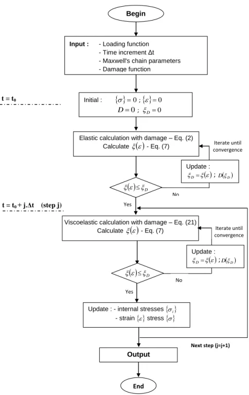
The incremental formulation presented above has been implemented as a numerical procedure using MATLAB® software. According to equations (21) or (23), the analysis is carried out in the form of a step-by-step procedure, which is divided in two successive parts:
- in a first part, the mechanical state of the structure is determined at the initial loading time. For an instant loading, the material behaves as damaging elastic. The calculation is iterated until convergence of the damage state in the material;
- in a second part, the analysis is divided in finite time steps Δt. Each step corresponds to a damaging viscoelastic analysis based on equation (21) or (23). In each viscoelastic step, the calculation is iterated until convergence of the damage state. Each step ends with the updating of the variables.
A detailed flow-chart of the incremental procedure is shown on Figure 1.
Figure 1 – Flow chart of the step-by-step procedure for the incremental analysis of a damaging viscoelastic structure
Begin
Input : - Loading function
- Time increment Δt
- Maxwell's chain parameters - Damage function
Elastic calculation with damage – Eq. (2) Calculate
- Eq. (7)
D
Viscoelastic calculation with damage – Eq. (21) Calculate
- Eq. (7)Update : - internal stresses
i - strain
stress
Output End t = t0 t = t0 + j.Δt (step j) Next step (j=j+1) Iterate until convergence No Yes Iterate until convergence No Yes Initial :
0 ;
0 D0 ; D0 Update : D ; D D Update : D ;D D
D 4.2 Damage function
The only requirement concerning the choice of a damage function is given by equation (4). In the following, a damage function proposed by Simo [3] is considered:
1
1
1
with
0
,
1
and
0
D D De
D
(25)
and Ω are scaling parameters :
1
is the scaling factor of the damage variable which gains increasing values between 0 and
1
in terms of the actual damage threshold
D. The rate of evolution ofD
D is controlled by the scaling factor Ω.5. Exemplary computations
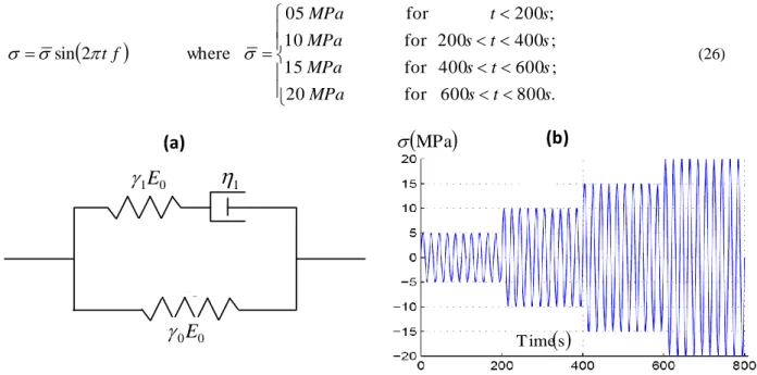
Two exemplary calculations are presented in order to illustrate the capabilities of the incremental formulation. In these two examples, a Zener model (Figure 2a) is used to represent the viscoelastic behaviour of the material with the following values for the material parameters:
GPa
30
0
E
;
0
.
2
;
0
0
.
3333
;
1
0
.
6667
; 1 10
.
25
s
5.1 One dimension analysis for a cyclic stress loading
In this example, the loading function consists of four sequences of ten alternate sinusoidal cycles each (Figure 2b). The loading frequency is
f
0
.
05
Hz
. The loading function is defined by
.
800
600
for
20
;
600
400
for
15
;
400
200
for
10
;
200
for
05
where
2
sin
s
t
s
MPa
s
t
s
MPa
s
t
s
MPa
s
t
MPa
f
t
(26)(a)
MPa
1
1E
0E
κ
1κ
0(b)
0 1E
s T ime 0 0E
Figure 2 – (a) Rheological Zener model (b) Stress loading versus time.
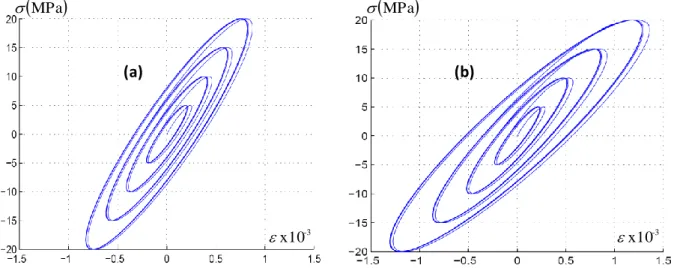
Figure 3a shows the evolution of the cyclic stress versus the computed cyclic strain in the case of a non-damaging viscoelastic material. The hysteresis is due to the delayed strain flow caused by the viscoelastic behaviour of the material, the dimensions of the hysteretic loops are proportional to the stress amplitude, but the tilt angle is constant, irrespective of the cyclic stress amplitude. Figure 3b presents the same evolution in the case of a damaging law. Compared with the previous case, the shapes of the hysteretic loops are modified by the damage in progress: the loops are broadened, and their inclination is increased with increasing value of the damage variable, leading therefore to larger cyclic strains than in the undamaging case. This feature is explained by the increase of damage which is based on the equivalent strain.
(b)
(a)
MPa
MPa
-3 x10
-3 x10
Figure 3 – Computed stress versus strain curves: (a) with
1
(no damage), (b) for
0
and
0
.
2
(with damage).5.2 Plane strain loading in 3D configuration
The second exemplary calculation concerns the 3D stress response to a plane strain loading defined as follows (Figure 4a):
constant
:
50
1
0
with
10
.
20
.
0
1
:
50
0
6t
s
t
t
t
s
t
-3x10
s T ime 1 2 1 2
Mpa
1
s T ime(b)
(a)
D 0.5 0.25 1 75 . 0 5 . 0 25 . 0 1 1 0 0 Figure 4 – (a) Strain loading
1 versus time. (b) Stress
1 and damage D versus time.Figure 4b presents the computed evolution of the first component of the stress tensor (
1- solid line) aside with the evolution of the damage variable (D - dashed line) for various fixed values of
. A relaxation in the stress state is observed as soon as the strain loading has reached its constant value. In all cases, higher values of
parameter yield higher values for the damage variable and the triaxial stress. This is due to the influence of the
2 strain component (
2
1) whose influence on
is increased when the
parameter is given a higher value, loading therefore to higher damage and weakened behaviour.7. Conclusion
An incremental formulation for the constitutive law of a damaging viscoelastic material has been developed in this paper. The formulation is based on a coupled damage viscoelastic model initially proposed by Simo [3]. The viscoelastic behaviour is represented by a generalized Maxwell’s chain. Based on [2], it was possible to turn the analytical coupled law into an incremental formulation. Taking advantage of this formulation, a step-by-step procedure has been implemented in MATLAB® software. The numerical procedure has been applied to two exemplary calculations: the one concerns the time analysis of a damaging viscoelastic material subjected to a uniaxial cyclic stress, the other concerns the same material subjected to a variable plane strain. In the first case, the strain amplitude is increased by the damaging process compared with the no-damage simulation. In the second case, the damage rate and the stress evolution are clearly influenced by the biaxiality of the applied strain. These two examples show the efficiency of the incremental approach. One main advantage of this approach is the fact that the time increment required for the step-by-step analysis needs be finite but not necessarily small. Therefore, the incremental formulation presented in this paper enables precise analysis of time dependent effects in complex structures for limited calculation efforts.
8. References
[1] Chang C.J., Sheng D.F. Quasi-static analysis for viscoelastic Timoshenko beams with damage. Appl Math Mech, 27(3), 295-304, 2006.
[2] Murakami S, et al. Computational methods for creep fracture analysis by damage mechanics. Comput Meth Appl Mech Eng, 183(1/2), 15-33, 2000.
[3] Simo J. On a fully three-dimensional finite-strain viscoelastic damage model: formulation and computational aspects. Comp Methods Appl Mech Eng, 60, 153-173, 1985.
[4] Zhao RG. Novel measuring approach for damage of viscoelastic material (Part I): Constitutive model. J. Cent. South Univ. Techn., s1−0289−04, 2007.
[5] Bhandari S. et al. Creep-damage analysis: comparison between coupled and uncoupled models. J Pressure Vessels Technol, 122(4), 408-12, 2000.
[6] Sullivan R.W. Development of a viscoelastic continuum damage model for cyclic loading. Mech Time-Depend Mater, 12, 329-342, 2008.
[7] Xicheng H. Damage theory for polymeric material. Appl Math Mech, 20(3), 338-342, 1999.
[8] Altenbach H, et al. Creep damage predictions in thin-walled structures by use of isotropic and anisotropic damage models. J Strain Anal Eng Des, 37(3), 265-275, 2002.
[9] Hyde T.H, et al. Finite element creep continuum damage mechanics analysis of pressurised pipe bends with ovality. JSME Int J, Ser A, 45(1):84-89, 2002.
[10] Kallmeyer A.R, Stephens R.I. A finite element model for predicting time-dependent deformations and damage accumulation in laminated composite bolted joints. J Compos Mater, 33(9), 794-826, 1999.
[11] Yue Z.F., Lu Z.Z. Finite element creep damage study of nickel base single crystal structures under multiaxial stress states. Mater Sci Technol, 19(8), 1012-1016, 2003.
[12] Jurkiewiez B., Destrebecq J.F., Vergne A. Incremental analysis of time-dependent effects in composite structures. Comp Struct, 73, 425-435, 1999.
[13] Destrebecq J.F., Jurkiewiez B. A numerical method for the analysis of rheologic effects in concrete bridges. Computer-Aided Civil and Infrastructure Engineering, 16(5), 347-364, 2001.
[14] Lemaitre J. Handbook of Materials Behavior Models. New York. Academic Press, 2001.