Approximate inference in Gaussian graphical models

(1)

by

Dmitry M. Malioutov

Submitted to the Department of Electrical Engineering and Computer Science in partial fulfillment of the requirements for the degree of

Doctor of Philosophy in

Electrical Engineering and Computer Science at the Massachusetts Institute of Technology

June, 2008 c

Signature of Author:

Department of Electrical Engineering and Computer Science May 23, 2008

Certified by:

Alan S. Willsky, Professor of EECS Thesis Supervisor

Accepted by:

Terry P. Orlando, Professor of Electrical Engineering Chair, Committee for Graduate Students

(2)

(3)

by Dmitry M. Malioutov

Submitted to the Department of Electrical Engineering and Computer Science on May 23, 2008

in Partial Fulfillment of the Requirements for the Degree

of Doctor of Philosophy in Electrical Engineering and Computer Science

Abstract

The focus of this thesis is approximate inference in Gaussian graphical models. A graphical model is a family of probability distributions in which the structure of interactions among the random variables is captured by a graph. Graphical models have become a powerful tool to describe complex high-dimensional systems specified through local interactions. While such models are extremely rich and can represent a diverse range of phenomena, inference in general graphical models is a hard problem.

In this thesis we study Gaussian graphical models, in which the joint distribution of all the random variables is Gaussian, and the graphical structure is exposed in the inverse of the covariance matrix. Such models are commonly used in a variety of fields, including remote sensing, computer vision, biology and sensor networks. Inference in Gaussian models reduces to matrix inversion, but for very large-scale models and for models requiring distributed inference, matrix inversion is not feasible.

We first study a representation of inference in Gaussian graphical models in terms of computing sums of weights of walks in the graph – where means, variances and corre-lations can be represented as such walk-sums. This representation holds in a wide class of Gaussian models that we call walk-summable. We develop a walk-sum interpretation for a popular distributed approximate inference algorithm called loopy belief propaga-tion (LBP), and establish condipropaga-tions for its convergence. We also extend the walk-sum framework to analyze more powerful versions of LBP that trade off convergence and accuracy for computational complexity, and establish conditions for their convergence. Next we consider an efficient approach to find approximate variances in large scale Gaussian graphical models. Our approach relies on constructing a low-rank aliasing matrix with respect to the Markov graph of the model which can be used to compute an approximation to the inverse of the information matrix for the model. By designing this matrix such that only the weakly correlated terms are aliased, we are able to give provably accurate variance approximations. We describe a construction of such a low-rank aliasing matrix for models with short-range correlations, and a wavelet-based construction for models with smooth long-range correlations. We also establish accuracy guarantees for the resulting variance approximations.

Thesis Supervisor: Alan S. Willsky

(4)

(5)

Symbol

Definition

General Notation

| · | absolute value

xi the ith component of the vector x

Xij element in the ith row and jth column of matrix X

(_·)T _{matrix or vector transpose}

(·)−1 _{matrix inverse}

det(_·) determinant of a matrix

tr(_·) trace of a matrix

R real numbers

RN vector space of real-valued N -dimensional vectors

I identity matrix

p(x) probability distribution of a random vector x pi(xi) marginal probability distribution of xi

p(x | y) conditional probability distribution of x given y

E[·] expected value

Ex[·] expected value, expectation is over p(x)

%(·) spectral radius of a matrix

Graph theory

G undirected graph

V vertex or node set of a graph

E edge set of a graph

|V | number of nodes, i.e. cardinality of the set V

2V set of all subsets of V

A_\B set difference

V\i all vertices except i, shorthand for V\{i} {i, j} an undirected edge in a graph (unordered pair) (i, j) a directed edge (ordered pair)

N (i) set of neighbors of node i

H hypergraph

F the collection of hyperedges in a hypergraph

(6)

Symbol

Definition

Graphical models ψi single-node potential ψij edge potential ψF factor potential Z normalization constant

F factor, a subset of nodes

xF subvector of x index by elements of F

mi→j message from i to j in BP

mA→i, mi→A messages in factor graph version of BP

∆J_i→j, ∆h_i→j messages in Gaussian BP ∆JA→i, ∆hA→i messages in Gaussian FG-LBP

T_i(n) n-step LBP computation tree rooted at node i

T_i(n)_→j n-step LBP computation tree for message m_i→j N (µ, P ) Gaussian distribution with mean µ and covariance P

J Information matrix for a Gaussian distribution

h potential vector for a Gaussian distribution

JF a submatrix of J indexed by F

[JF] JF zero-padded to have size N× N

λmin(J) smallest eigenvalue of J

rij partial correlation coefficient

Walk-sums

R partial correlation matrix

¯

R matrix of elementwise absolute values of R

w a walk

w : i_{→ j} set of walks from i to j

w :_{∗ → j} set of walks that start anywhere and end at j w : i_{→ j}l set of walks from i to j of length l

φ(w) weight of a walk

W a collection of walks

W(i → i) self-return walks

W(i→ i)\i single-revisit self-return walks W(∗→ i)\i single-visit walks

(7)

Symbol

Definition

walk-sums (continued)

φ(_W) walk-sum

φ(i_{→ i)} self-return walk-sum φh(W) input reweighted walk-sum

R(n)_i partial correlation matrix for computation tree T_i(n) %_∞ limit of the spectral radius of R(n)_i

QG set of block-orthogonal matrices on G

SG set of block-invertible matrices on G

¯

φk a matrix of absolute walk-sums for walks of length k

Low-rank variance approximation ˆ

P approximation of P

Pi ith column of P

vi ith standard basis vector

BBT _{low-rank aliasing matrix}

B a spliced basis

bi ith row of B corresponding to node i

Bk kth column of B

Rk solution to the system JRk= Bk

σi random sign for node i

E error in covariance, ˆP − P

C(i) set of nodes of the same color as i V ar(_·) variance of a random variable φs,k(t) kth wavelet function at scale s

ψs,k(t) kth scaling function at scale s

(8)

(9)

I have been very fortunate to work under the supervision of Professor Alan Willsky in the wonderful research environment that he has created in the Stochastic Systems Group. Alan’s deep and extensive knowledge and insight, energy, enthusiasm, and the ability to clearly explain even the most obscure concepts in only a few words are re-markable and have been very inspiring throughout the course of my studies. There are too many reasons to thank Alan – from providing invaluable guidance on research, and allowing the freedom to explore topics that interest me the most, to financial support, to giving me an opportunity to meet and interact with world-class researchers through SSG seminars and sending me to conferences1, and finally for the extremely prompt and yet very careful review process of my thesis. I would like to thank my commit-tee members, Professor Pablo Parrilo, and Professor William Freeman, for suggesting interesting research directions, and for detailed reading of my thesis.

It has been a very rewarding experience interacting with fellow students at SSG – from discussing and collaborating on research ideas, and providing thoughtful criticism and improvements of papers and presentations, to relaxing after work. In particular I’d like to thank Jason Johnson who has been my office-mate throughout my graduate stud-ies. Much of the work in this thesis has greatly benefited from discussions with Jason – he has always been willing to spend time and explain topics from graphical models, and he has introduced me to the walk-sum expansion of the inverse of the information matrix, which has lead to exciting collaboration the product of which now forms the bulk of my thesis. In addition to research collaboration, Jason has become a good friend, and among a variety of other things he introduced me to the idea of sparsifying some of the ill-formed neural connections by going to the Muddy on Wednesdays, and taught me the deadly skill of spinning cards. I would also like to thank Sujay Sanghavi for generously suggesting and collaborating on a broad range of interesting ideas, some of which have matured into papers (albeit, on topics not directly related to the title of this thesis). I also acknowledge interactions with a number of researchers both at MIT and outside. I would like to thank Devavrat Shah, David Gamarnik, Vivek Goyal, Venkatesh Saligrama, Alexander Postnikov, Dimitri Bertsekas, Mauro Maggioni, Alfred Hero, Mujdat Cetin, John Fisher, Justin Dauwels, Eric Feron, Mardavij Roozbehani, Raj Rao, Ashish Khisti, Shashi Borade, Emin Martinian, and Dmitry Vasiliev. I es-pecially would like to thank Hanoch Lev-Ari for interesting discussions on relation of walk-sums with electrical circuits. I learned a lot about seismic signal processing from 1_{Although for especially exotic locations, such as Hawaii, it sometimes took quite a bit of convincing}

why the submitted work was innovative and interesting.

(10)

Jonathan Kane and others at Shell. Also I greatly enjoyed spending a summer working on distributed video coding at MERL under the supervision of Jonathan Yedidia and Anthony Vetro. I would like to thank my close friends Gevorg Grigoryan and Nikolai Slavov for ongoing discussions on relations of graphical models and biology.

My years at MIT have been very enjoyable thanks in large part to the great fellow students at SSG. I would like to thank Jason Johnson, Ayres Fan and Lei Chen for making our office such a pleasant place to work, or rather a second home, for a number of years. Special thanks to Ayres for help with the many practical sides of life including the job search process and (in collaboration with Walter Sun) for teaching me not to keep my rubles under the pillow. I very much enjoyed research discussions and playing Hold’em with Venkat Chandrasekaran, Jin Choi, and Vincent Tan. Vincent – a day will come when I will, with enough practice, defeat you in ping-pong. Thanks to Kush Varshney for eloquently broadcasting the news from SSG to the outside world, to Pat Kreidl and Michael Chen for their sage, but very contrasting, philosophical advice about life. Thanks to our dynamite-lady Emily Fox for infusing the group with lively energy, and for proving that it is possible to TA, do research, cycle competitively, play hockey, and serve on numerous GSC committees all at the same time. Thanks to the student-forever Dr. Andy Tsai for gruesome medical stories during his brief vacations away from medical school which he chose to spend doing research at SSG. I also enjoyed interacting with former SSG students – Walter Sun, Junmo Kim, Eric Sudderth, Alex Ihler, Jason Williams, Lei Chen, Martin Wainwright and Dewey Tucker. Many thanks to Brian Jones for timely expert help with computer and network problems, and to Rachel Cohen for administrative help.

During my brief encounters outside of SSG I have enjoyed the company of many students at LIDS, CSAIL, and greater MIT. Many thanks for the great memories to the 5-th floor residents over the years, in particular the french, the italians (my tortellini-cooking friends Riccardo, Gianbattista, and Enzo), the exotic singaporeans (big thanks to Abby for many occasions), and the (near)-russians, Tolya, Maksim, Ilya, Evgeny, Nikolai, Michael, Grisha. Thanks to Masha and Gevorg for being great friends, and making sure that I do not forget to pass by the gym or the swimming pool once every few weeks. Many thanks for all my other russian friends for good times and for keeping my accent always strong. I was thrilled to learn brazilian rhythms, and even occasionally perform, with Deraldo Ferreira, and his earth-shaking samba tremeterra, and Marcus Santos. I would especially like to thank Wei for her sense of humour, her fashion advice, and in general for being wonderful.

Finally I thank all of my family, my MIT-brother Igor, and my parents for their constant support and encouragement. I dedicate this thesis to my parents.

(11)

Introduction

Analysis and modeling of complex high-dimensional data has become a critical research problem in the fields of machine learning, statistics, and many of their applications. A significant ongoing effort has been to develop rich classes of statistical models that can represent the data faithfully, and at the same time allow tractable learning, esti-mation and sampling. Graphical models [13, 35, 78, 83] constitute a powerful framework for statistical modeling that is based on exploiting the structure of conditional indepen-dence among the variables encoded by a sparse graph. Certain examples of graphical models have been in use for quite a long time, but recently the field has been gaining momentum and reaching to an ever increasing and diverse range of applications.

A graphical model represents how a complex joint probability distribution decom-poses into products of simple local functions (or factors) that only depend on small subsets of variables. This decomposition is represented by a graph: a random variable is associated with each vertex, and the edges or cliques represent the local functions. An important fact that makes the framework of graphical models very powerful is that the graph captures the conditional independence structure among the random variables. It is the presence of this structure that enables the compact representation of rich classes of probability models and efficient algorithms for estimation and learning. The applica-tions of graphical models range from computer vision [51,100,121], speech and language processing [14, 15, 114], communications and error control coding [29, 52, 55, 91], sensor networks [24, 66, 96], to biology and medicine [54, 84, 137], statistical physics [93, 104], and combinatorial optimization [94, 112]. The use of graphical models has led to revo-lutionary advances in many of these fields.

The graph in the model is often specified by the application: in a genomic applica-tion the variables may represent expression levels of certain genes and the edges may represent real biological interactions; in computer vision the nodes may correspond to pixels or patches of an image and the edges may represent the fact that nearby nodes are likely to be similar for natural images. The graph may also be constructed for the purpose of efficiency: e.g., tree-structured and multiscale models allow particularly efficient estimation and learning [33,135]. In this case nodes and edges may or may not have direct physical meaning. The use of graphical models involves a variety of tasks – from defining or learning the graph structure, optimizing model parameters given data, finding tractable approximations if the model is too complex, sampling configurations

(16)

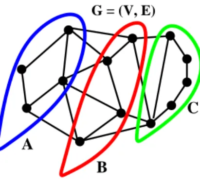
G = (V, E)

B

C A

Figure 1.1. Markov property of a graphical model: graph separation implies conditional independence.

of the model, and finally doing inference – estimating the states of certain variables given possibly sparse and noisy observations. In this thesis we focus mostly on the last problem – doing inference when the model is already fully defined. This is an important task in and of itself, but in addition inference can also be an essential part of learning and sampling.

Graphical models encompass constructions on various types of graphs (directed and undirected, chain-graphs and factor-graphs), and in principle have no restrictions on the state-space of the random variables – the random variables can be discrete, continuous, and even non-parametric. Of course, with such freedom comes responsibility – the most general form of a graphical model is utterly intractable. Hence, only certain special cases of the general graphical models formalism have been able to make the transition from theory into application.

¥ 1.1 Gaussian Graphical Models

In this thesis we focus on Gaussian graphical models, where the variables in the model are jointly Gaussian. Also, for the most part we restrict ourselves to Markov random fields (MRF), i.e. models defined on undirected graphs [110]. We will use acronyms Gaussian graphical model (GGM) and Gaussian Markov random field (GMRF) inter-changeably. These models have been first used in the statistics literature under the name covariance selection models [43, 115]. A well-known special case of a GGM is a linear state-space model – it can be represented as a graphical model defined on a chain. As for any jointly Gaussian random variables, it is possible to write the probability density in the conventional form:

p(x) = 1

p(2π)N_{det(P )}−1exp(−

1

2(x− µ)

T_P−1_(x_{− µ))} _(1.1)

where the mean is µ = E[x], and the covariance matrix is P = E[xxT_{]. What makes the}

(17)

...

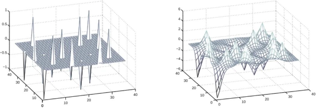
0 10 20 30 40 50 60 70 80 90 100 0 10 20 30 40 50 60 70 80 90 100 −100 −50 0 50 100

Figure 1.2. (a) A GMRF on a grid graph. (b) A sample from the GMRF.

also called the Markov structure, which is captured by a graph. Given a Markov graph of the model the conditional independence relationships can be immediately obtained. Consider Figure 1.1. Suppose that removing a set of nodes B separates the graph into two disconnected components, A and C. Then the variables xAand xC (corresponding

to nodes in A and C) are conditionally independent given xB. This generalizes the

well-known property for Markov chains: the past is independent of the future given the current state (removing the current state separates the chain into two disconnected components).

For GGM the Markov structure can be seamlessly obtained from the inverse covari-ance matrix J , P−1_{, also called the information matrix. In fact, the sparsity of J}

exactly matches the Markov graph of the model: if an edge_{{i, j} is missing from the} graph then Jij = 0. This has the interpretation that xi and xj are conditionally

inde-pendent given all the other variables in the model. Instead of (1.1) we will extensively use an alternative representation of a Gaussian probability density which reveals the Markov structure, which is parameterized by J = P−1 and h = Jµ. This representation is called the information form of a Gaussian density with J and h being the information parameters:

p(x)∝ exp(−1 2x

T_{Jx + h}T_x) _(1.2)

GMRF models are used in a wide variety of fields – from geostatistics, sensor net-works, and computer vision to genomics and epidemiological studies [27, 28, 36, 46, 96, 110]. In addition, many quadratic problems arising in machine learning and optimiza-tion may be represented as Gaussian graphical models, thus allowing to apply methods developed in the graphical modeling literature [10, 11, 128]. To give an example of how a GMRF might be used we briefly mention the problem of image interpolation from sparse noisy measurements. Suppose the random variables are the gray-levels at each

(18)

0 20 40 60 80 100 −3 −2 −1 0 1 2 3 0 20 40 60 80 100 −0.2 0 0.2 0.4 0.6 0.8 0 20 40 60 80 100 −4 −3 −2 −1 0 1 2 3 4 0 20 40 60 80 100 0 0.5 1 1.5

Figure 1.3. Samples from a chain GMRF, and the correlations between the center node and the other nodes.

of the pixels in the image, and we use the thin-plate model which captures smoothness properties of natural images (we discuss such models in more detail in Chapter 2). The Markov graph for the thin-plate model is a grid with connections up to two steps away, see Figure 1.2 (a). In Figure 1.2 (b) we show a random sample from this model, which looks like a plausible geological surface. A typical application in geostatistics would try to fit model parameters such that the model captures a class of surfaces of interest, and then given a sparse set of noisy observations interpolate the surface and provide error variances. For clarity we show a one-dimensional chain example in Figure 1.3. In the top left plot we show a number of samples from the prior, and in the top right plot we show several conditional samples given a few sparse noisy measurements (shown in cir-cles). The bottom left plot displays the long correlation in the prior model (between the center node and the other nodes), and the bottom right plot shows that the posterior variances are smallest near the measurements.

As we discuss in more detail in Chapter 2 the prior model p(x) specifies a sparse J matrix. Adding local measurements of the form p(y|x) = Q p(yi|xi), the posterior

becomes p(x_{|y) ∝ p(y|x)p(x). The local nature of the measurements does not change} the graph structure for the posterior – it only changes the diagonal of J and the h-vector.

¥ 1.2 Inference in Gaussian Models

Given a GGM model in information form, we consider the problem of inference (or estimation) – i.e. determining the marginal densities of the variables given some

(19)

ob-servations. This requires computing marginal means and variances at each node. In principle, both means and variances can be obtained by inverting the information ma-trix: P = J−1 and µ = P h. The complexity of matrix inversion is cubic in the number of variables, so it is appropriate for models of moderate size. More efficient recursive calculations are possible in graphs with very sparse structure—e.g., in chains, trees and in graphs with “thin” junction trees [83] (see Chapter 2). For these models, belief propagation (BP) or its junction tree variants [35,103] efficiently compute the marginals in time linear in the number of variables1_{. In large-scale models with more complex}

graphs, e.g. for models arising in oceanography, 3D-tomography, and seismology, even the junction tree approach becomes computationally prohibitive. Junction-tree versions of belief propagation reduce the complexity of exact inference from cubic in the num-ber of variables to cubic in the “tree-width” of the graph [83]. For square and cubic lattice models with N nodes this leads to complexity O(N3/2) and O(N2) respectively. Despite being a great improvement from brute-force matrix inversion, this is still not scalable for large models. In addition, junction-tree algorithms are quite involved to implement. A recent method, recursive cavity modeling (RCM) [76], provides tractable computation of approximate means and variances using a combination of junction-tree ideas with recursive model-thinning. This is a very appealing approach, but analytical guarantees of accuracy have not yet been established, and the implementation of the method is technically challenging. We also mention a recently developed Lagrangian relaxation (LR) method which decomposes loopy graphs into tractable subgraphs and uses Lagrange dual formulation to enforce consistency constraints among them [73, 75]. LR can be applied to both Gaussian and discrete models, and for the Gaussian case it computes the exact means and provides upper bounds on the variances.

Iterative and multigrid methods from numerical linear algebra [126, 127] can be used to compute the marginal means in a sparse GMRF to any desired accuracy, but these methods do not provide the variances. In order to also efficiently compute vari-ances in large-scale models, approximate methods have to be used. A wide variety of approximate inference methods exists which can be roughly divided into variational in-ference [95,131,136] and Monte Carlo sampling methods [57,108]. In the first part of the thesis we focus on an approach called loopy belief propagation (LBP) [103,111,133,138], which iteratively applies the same local updates as tree-structured belief propagation to graphs with loops. It falls within the realm of variational inference. We now briefly motivate LBP and tree-structured exact BP. Chapter 2 contains a more detailed pre-sentation.

(20)

i m

ij

j

Figure 1.4. BP figure.

¥ 1.3 Belief Propagation: Exact and Loopy

In tree-structured models belief propagation (or the sum-product algorithm) is an exact message-passing algorithm to compute the marginals2_{. It can be viewed as a form of}

variable elimination – integrating out the variables one by one until just the variable of interest remains. To naively compute all the marginals, simple variable elimination would have to be applied for each variable, producing a lot of redundant repeated computations. Belief propagation eliminates this redundancy by processing all variables together and storing the intermediate computations as messages. Consider Figure 1.4: a message mij from i to j captures the effect of eliminating the whole subtree that

extends from i in the direction away from j – this message will be used to compute all the marginals to the right of node i. By passing these messages sequentially from the leaves to some designated root and back to the leaves, all marginals can be computed in O(N ) message updates. Message updates can also be done in parallel: all messages are first initialized to an uninformative value, and are repeatedly updated until they reach a fixed point. In tree-structured models parallel form of updates is also guaranteed to converge and provide the correct marginals after a fixed number of iterations.

Variable elimination corresponds to simple message updates only in tree-structured graphs. In presence of loops it modifies the graph by introducing new interactions (edges) among the neighbors of the eliminated variables. This can be resolved by merging variables together until the graph becomes a tree (form a junction tree), but, as we mentioned, for grids and denser graphs this quickly becomes computationally intractable.

Alternatively, one could ignore the loops in the graph and still carry out local BP message updates in parallel until they (hopefully) converge. This approach is called loopy belief propagation (LBP). LBP has been shown to often provide excellent approx-imate solutions for many hard problems, it is tractable (has a low cost per iteration) and allows distributed implementation, which is crucial in applications such as sensor networks [96]. However, in general it ’double counts’ messages that travel multiple 2_{A version of belief propagation called max-product also addresses MAP estimation, but for Gaussian}

(21)

times around loops which may in certain cases give very poor approximations, and it is not even guaranteed to converge [101].

There has been a significant effort to explain or predict the success of LBP for both discrete and Gaussian models: in graphs with long loops and weak pairwise interactions, errors due to loops will be small; the binary MRF max-product version of loopy belief propagation is shown to be locally optimal with respect to a large set of local changes [134] and for the weighted matching problem the performance of LBP has been related to that of linear programming relaxation [112]; in GMRFs it has been shown that upon convergence the means are correct [129, 133]; sufficient conditions for LBP convergence are given in [69, 99, 124]; and there is an interpretation of loopy belief propagation fixed points as being stationary points of the Bethe-free energy [138]. However despite this progress, the understanding of LBP convergence and accuracy is very limited, and further analysis is an ongoing research effort. Analysis of LBP using the walk-sum framework for Gaussian inference [74, 86] is the subject of Chapters 3 and 4 of this thesis. This analysis provides much new insight into the operation of Gaussian LBP, gives the tightest sufficient conditions for its convergence, and suggests when LBP may be a suitable algorithm for a particular application.

There are some scenarios where the use of LBP to compute the variances is less than ideal (e.g. for models with long-range correlations): either LBP fails to converge or converges excruciatingly slowly or gives very inaccurate approximations for the vari-ances. In Chapter 5 we propose an efficient method for computing accurate approximate variances in very large scale Gaussian models based on low-rank approximations.

¥ 1.4 Thesis Contributions

This thesis makes two main contributions: a graph-theoretic framework for interpreting Gaussian loopy belief propagation in terms of computing walk-sums and new results on LBP convergence and accuracy, and a low-rank approach to compute accurate approxi-mate variances in large-scale GMRF models. We now introduce these two contributions in more detail.

¥ 1.4.1 Walk-sum Analysis of Loopy Belief Propagation

We first describe an intuitive graphical framework for the analysis of inference in Gaus-sian models. It is based on the representation of the means, variances and correlations in terms of weights of certain sets of walks in the graph. This ’walk-sum’ formulation of Gaussian inference originated from a course project in [72] and is based on the Neumann series (power-series) for the matrix inverse:

P = J−1= (I_{− R)}−1 =

∞

X

k=0

Rk, if ρ(R) < 1. (1.3)

Suppose that J is the normalized (unit-diagonal) information matrix of a GMRF, then R is the sparse matrix of partial correlation coefficients which has zero-diagonal, but

(22)

the same off-diagonal sparsity structure as J. As we discuss in Chapter 3, taking k-th power of R corresponds to computing sums of weights of walks of length k. And we show that means, variances, and correlations are walk-sums (sums of weights of the walks) over certain infinite sets of walks.

This walk-sum formulation applies to a wide class of GMRFs for which the expansion in (1.3) converges (if the spectral radius satisfies ρ(R) < 1). However, we are interested in a stricter condition where the result of the summation is independent of its order – i.e. the sum over walks converges absolutely. We call models with this property walk-summable. We characterize the class of walk-summable models and show that it contains (and extends well beyond) some “easy” classes of models, including models on trees, attractive, non-frustrated, and diagonally dominant models. We also show that walk-summability is equivalent to the fundamental notion of pairwise-normalizability.

We use the walk-sum formulation to develop a new interpretation of BP in trees and of LBP in general. Based on this interpretation we are able to extend the previously known sufficient conditions for convergence of LBP to the class of walk-summable mod-els. Our sufficient condition is tighter than that based on diagonal dominance in [133] as walk-summable models are a strict superset of the class of diagonally dominant models, and as far as we know is the tightest sufficient condition for convergence of Gaussian LBP3.

We also give a new explanation, in terms of walk-sums, of why LBP converges to the correct means but not to the correct variances. The reason is that LBP captures all of the walks needed to compute the means but only computes a subset of the walks needed for the variances. This difference between means and variances comes up because of the mapping that assigns walks from the loopy graph to the so-called LBP computation tree: non-backtracking walks (see Chapter 3) in the loopy graph get mapped to walks that are not ’seen’ by LBP variances in the computation tree.

In general, walk-summability is sufficient but not necessary for LBP convergence. Hence, we also provide a tighter (essentially necessary) condition for convergence of LBP variances based on a weaker form of walk-summability defined on the LBP computation tree. This provides deeper insight into why LBP can fail to converge—because the LBP computation tree is not always well-posed.

In addition to scalar walk-summability we also consider the notions of vector and factor-graph walk-summability, and vector and factor-graph normalizability. Any Gaus-sian model can be perfectly represented as a scalar pairwise MRF, but using LBP on equivalent scalar and factor-graph models gives very different approximations. Using factor-graph models with larger factors provides the flexibility of being able to trade off complexity versus accuracy of approximation. While many of our scalar results do 3_{In related work [97] (concurrent with [86]) the authors make use of our walk-sum analysis of LBP,}

assuming pairwise-normalizability, to consider other initializations of the algorithm. Here, we choose one particular initialization of LBP. However, fixing this initialization does not in any way restrict the class of models or applications for which our results apply. For instance, the application considered by [96] can also be handled in our framework by a simple reparameterization. However, the critical condition is still walk-summability, which is presented in [86].

(23)

0 10 20 30 40 0 10 20 30 40 −1 −0.5 0 0.5 1 0 10 20 30 40 0 10 20 30 40 −6 −4 −2 0 2 4 6

Figure 1.5. Aliasing of the covariance matrix in a 2D GMRF model. For large-scale GMRF models this allows tractable computation of approximate variances.

carry over to these more general conditions, some of the results become more involved and many interesting open questions remain.

The intuitive interpretation of correlations as walk-sums for Gaussian models begs the question of whether related walk-sum interpretation exists for other graphical mod-els. While the power-series origin of the walk-sum expansion (1.3) is limited to Gaussian models, related expansions (over paths, self-avoiding walks, loops, or subgraphs) have been developed for other types of models [23,30,49,77,122], and exploring possible con-nections to Gaussian walk-sums is an exciting direction for further work. In addition, Gaussian walk-sums have potentials to develop new algorithms which go beyond LBP and capture more of the variance-walks in loopy graphs. We suggest these and other directions for further research in Chapter 6 of the thesis.

¥ 1.4.2 Variance Approximation

Error variances are a crucial component of estimation, providing the reliability infor-mation for the means. They are also useful in other respects: regions of the field where residuals exceed error variances may be used to detect and correct model-mismatch (for example when smoothness models are applied to fields that contain abrupt edges). Also, as inference is an essential component of learning a model (for both parameter and structure estimation), accurate variance computation is needed when designing and fitting models to data. Another use of variances is to assist in selecting the location of new measurements to maximally reduce uncertainty.

We have already discussed the difficulties of computing the variances in large-scale models: unless the model is ’thin’, exact computations are intractable. The method of loopy belief propagation can be a viable solution for certain classes of models, but in models with long-range correlations it either does not converge at all, or gives poor approximations.

(24)

theo-retical guarantees of accuracy. In our approach we use a low-rank aliasing matrix to compute an approximation to the inverse J−1 = P . By designing this matrix such that only the weakly correlated terms are aliased (see Figure 1.5), we are able to give prov-ably accurate variance approximations. We propose a few different constructions for the low-rank matrix. We start with a design for single-scale models with short correlation length, and then extend it to single-scale models with long correlation length using a wavelet-based aliasing matrix construction. GMRFs with long correlation lengths, e.g. fractional Gaussian noise, are often better modeled using multiple scales. Thus we also extend our wavelet based construction to multi-scale models, in essence making both the modeling and the processing multi-scale.

¥ 1.5 Thesis Outline

We start by providing a more detailed introduction to graphical models and GMRF models in Chapter 2. We discuss directed and undirected models and factor-graph formulations, and provide a detailed discussion of LBP and the computation-tree in-terpretation of LBP. In Chapter 3 we describe the walk-sum framework for Gaussian inference, and use it to analyze the LBP algorithm for Gaussian models, providing the best known sufficient conditions for its convergence. In Chapter 4 we generalize the walk-sum framework to vector and factor-graph models, and extend some of the re-sults from the scalar ones. We also outline certain combinatorial ideas for computing walk-sums. In Chapter 5 we move on to describe the low-rank approach to compute approximate variances in large-scale GMRF models. We first describe the time-domain short-correlation approach, and then describe the wavelet-based long-range correlation version. In Chapter 6 we discuss open problems and suggestions for further work.

Bibliographic notes Parts of this thesis are based on our publications [74, 85–88] re-flecting research done in collaboration with J. Johnson.

(25)

Background

In this chapter we give a brief self-contained introduction to graphical models, includ-ing factorizations of probability distributions, their representations by graphs, and the Markov (conditional independence) properties. We start with general graphical models in Section 2.1, and then specialize to the Gaussian case in Section 2.3. We outline ap-proaches to inference in graphical models, both exact and approximate. We summarize exact belief propagation on trees and the junction tree algorithm in Section 2.2, and the approximate loopy belief propagation on general graphs in Section 2.2.2.

¥ 2.1 Preliminaries: Graphical Models

In this Section we formalize the concept of a graphical model, describe several types of graphical model such as MRFs, factor graphs and Bayesian networks, their graphical representation, and the implied conditional independence properties. First we briefly review some basic notions from graph theory [8, 12, 16], mainly to fix notation.

¥ 2.1.1 Graph Theory

A graph G = (V,E) is specified as a collection of vertices (or nodes) V together with a collection of edges_{E ⊂ V × V , i.e. E is a subset of all pairs of vertices. In this thesis we} mostly deal with simple undirected graphs, which have no self-loops, and at most one edge between any pair of vertices. For undirected edges we use the set notation {i, j} as the ordering of the two vertices does not matter. Unless we state otherwise, we will assume by default that all edges are undirected. In case we need to refer to directed edges we use the ordered pair notation (i, j).

The neighborhood of a vertex i in a graph is the set _{N (i) = {j ∈ V | {i, j} ∈ E}.} The degree of a vertex i is its number of neighbors_{|N (i)|. A graph is called k-regular} if the degree of every vertex is k. A subgraph of G is a graph Gs = (Vs,Es), where

Vs ⊂ V , and Es ⊂ Vs× Vs. We also say that G is a supergraph of Gs and that Gs is

embedded in G. A clique of G is a fully connected subgraph of G, i.e. _{C = (V}s,Es) with

every pair of vertices connected: i, j ∈ Vs ⇒ {i, j} ∈ Es. A clique is maximal if it is

not contained within another clique. A walk w in a graph G is a sequence of vertices w = (w0, w1, ..., wl), wi∈ V , where each pair of consequent vertices is connected by an

edge, {wi, wi+1} ∈ E. The length of the walk is the number of edges that it traverses;

(26)

the walk w in our definition has length l. A path is a walk where all the edges and all the vertices are distinct. A graph is called connected if there is a path between any two vertices. The diameter of a graph diam(G) is the maximum distance between any pair of vertices, where distance is defined as the length of the shortest path between the pair of vertices.

A chain is a connected graph where two of the vertices have one neighbor each, and all other vertices have two neighbors. A cycle is a connected graph, where each vertex has exactly two neighbors. A tree is a connected graph which contains no cycles as subgraphs. A graph is called chordal if every cycle of the graph which has length 4 or more contains a chord (an edge between two non-adjacent vertices of the cycle). The treewidth of a graph G is the minimum over all chordal graphs containing G of the size of the largest clique in the chordal graph minus one. As we explain later, treewidth of a graph is a measure of complexity of exact inference for graphical models.

A hypergraph _{H = (V, F) is a generalization of an undirected graph which allows} hyper-edges F ∈ F connecting arbitrary subsets of vertices, rather than just pairs of vertices. HereF ⊂ 2V _{is a collection of hyper-edges, i.e. arbitrary subsets of V .}

¥ 2.1.2 Graphical Representations of Factorizations of Probability

Graphical models are multivariate statistical models defined with respect to a graph. The main premise is that the joint density of a collection of random variables can be expressed as a product of several factors, each depending only on a small subset of the variables. Such factorization induces a structure of conditional independence among the variables. The graph encodes the structure of these local factors, and, importantly, it gives a very convenient representation of the conditional independence properties, thus enabling efficient algorithms which have made graphical models so popular.

There are various ways to use graphs to represent factorizations of a joint density into factors: Bayesian networks are based on directed graphs [35, 71], Markov random fields (MRF) are based on undirected graphs [9, 28, 110], and factor graphs [82] use hypergraphs (encoded as bipartite graphs with variable and factor nodes). We now describe these graphical representation of factorization, and how they relate to condi-tional independence properties of the graphical model. We focus on factor graph and MRF representation first, and later comment on their relation to the directed (Bayesian network) representation.

Suppose that we have a vector of random variables, x = (x1, x2, ..., xN) with

discrete or continuous state space xi ∈ X . Suppose further that their joint density

p(x) can be expressed as a product of several positive functions (also called factors or potentials1) ψF ≥ 0, indexed by subsets F ⊂ {1, .., N} over some collection F ∈ F.

Each of the functions ψF only depends on the subset of random variables in F , i.e.

1_{To be precise, it is actually the negative logarithms of ψ}

F that are usually referred to as potentials

(27)

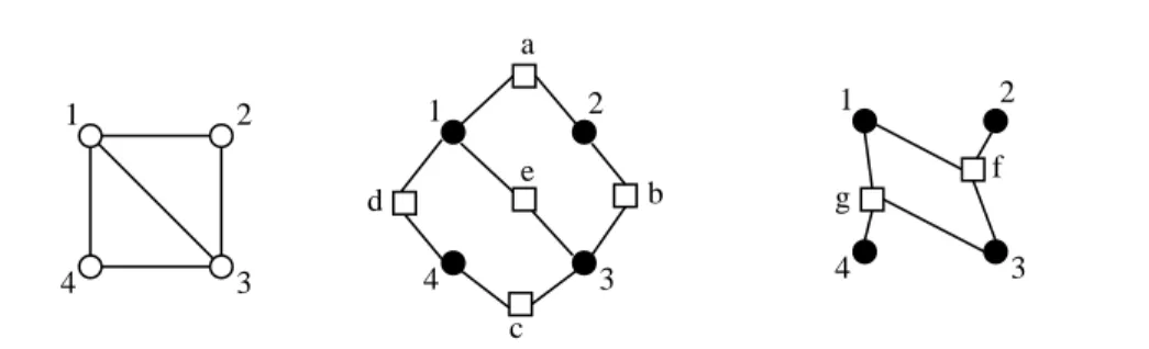
3 4 1 2 3 4 1 2 a b c e d f g 2 3 4 1

Figure 2.1. An undirected graph representation and two possible factor graphs corresponding to it. See Exaple 1 for an explanation.

ψF = ψF(xF), where we use xF to denote the variables in F , i.e. xF ={xi, i∈ F }:

p(x) = 1 Z

Y

F∈F

ψF(xF), F ∈ F. (2.1)

Z is a normalizing constant, also called the partition function, which makes p(x) in-tegrate (or sum) to 1, Z = P

x

Q

F∈FψF(xF), F ∈ F. Typically the factors ψF

depend only on a small subset of variables, _{|F | ¿ |V |, and a complicated probability} distribution over many variables can be represented simply by specifying these local factors.

A factor graph summarizes the factorization structure of p(x) by having two sets of vertices: variable-nodes Vv = {1, ..., N} and factor-nodes Vf ={1, ..., |F|}. The graph

has an edge between a variable-node i_{∈ V}v and a factor-node F ∈ Vf if i∈ F , i.e. if

ψF does depend on xi. The factor graph has no other edges2. Two examples with 4

variables are displayed in Figure 2.1, middle and right plots, with circles representing variables and squares representing the factors.

Another way to encode the structure of p(x) is using undirected graphs, G = (V,_E), which is referred to as the Markov random field (MRF) representation. Each vertex i corresponds to a random variable xi, and an edge {i, j} appears between nodes i and j

if some factor ψF depends on both xiand xj. It is clear that each subset F ∈ F of nodes

is a clique in G. Thus instead of using special factor-nodes, an MRF representation encodes factors by cliques. However, the representation is somewhat ambiguous as some cliques may not correspond to a single factor but to several smaller factors, which together cover the clique. Hence, the fine details of the factorization of p(x) in (2.1) may not be exposed just from the undirected graph and only become apparent using a factor graph representation. We explain these ideas in Example 1 below. The undirected graph representation is however very convenient in providing the Markov (conditional independence) properties of the model.

The mapping from the conditional independence properties of an MRF model to the structure of the graph comes from the concept of graph separation. Suppose that the

2_{A factor graph is bipartite: the vertices are partitioned into two sets V}

v and Vf, and every edge

(28)

set of nodes is partitioned into three disjoint sets V = A_{∪ B ∪ C. Then B separates A} from C if any path from a vertex in A to a vertex in C has to go through some vertex in B. A distribution p(x) is called Markov with respect to G if for any such partition, xA

is independent of xC given xB, i.e. p(xA, xC|xB) = p(xA|xB)p(xC|xB). The connection

between factorization and the Markov graph is formalized in the theorem of Hammersley and Clifford (see [21, 59, 83] for a proof):

Theorem 2.1.1 (Hammersley-Clifford Theorem). If p(x) = _Z1 Q

F∈FψF(xF) with

ψF(xF)≥ 0, then p(x) is Markov with respect to the corresponding graph G. Conversely,

if p(x) > 0 for all x, and p(x) is Markov with respect to G, then p(x) can be expressed as a product of factors corresponding to cliques of G.

Example 1 To illustrate the interplay of density factorization, Markov properties and factor graph and MRF representation, consider the undirected graph in Figure 2.1 on the left. The graph is a 4-node cycle with a chord. The absence of the edge{2, 4} implies that for any distribution that is Markov with respect to G, x2 and x4 are independent

given x1 and x3. However, x2 and x4 are not independent given x1 alone, since there is

a path (2, 3, 4) which connects them, and does not go through x1.

The graph has two maximal cliques of size 3: {1, 2, 3}, and {1, 3, 4}, and five cliques of size 2: one for each of the edges. By Hammersley-Clifford theorem, any distri-bution that is Markov over this graph is a product of factors over all the cliques. However, for a particular distribution some of these factors may be trivially equal to 1 (and can be ignored). Hence, there may be a few different factor graphs associ-ated with this graph. Two possibilities are illustrassoci-ated in Figure 2.1, center plot, with p(x) = ψa(x1, x2)ψb(x2, x3)ψc(x3, x4)ψd(x1, x4)ψe(x1, x3), and right plot with p(x) =

ψf(x1, x2, x3)ψg(x1, x3, x4). The variable-nodes are denoted by circles, and the

factor-nodes are denoted by squares. The example shows that the undirected representation is useful in obtaining the Markov properties, but a factor graph can serve as a more accurate (more restrictive) representation of the factorization. ¤

It is convenient to restrict attention to models with pairwise interactions – i.e. models where all the factors depend on at most two variables (i.e. all ψF satisfy|F | ≤ 2,

for example see Figure 2.1 middle plot). By merging some of the variables together (thereby increasing the state space) any MRF can be converted into a pairwise MRF. In the sequel, unless stated otherwise, we use pairwise MRFs. When dealing only with pairwise MRFs there is little benefit in using the factor graph representation, since it does nothing except adding factor-nodes in the middle of every edge. An MRF representation carries exactly the same information for the pairwise case. The factorization of a density for a pairwise MRF has the following form:

p(x) = 1 Z Y i∈V ψi(xi) Y {i,j}∈E ψi,j(xi, xj) (2.2)

(29)

Tree-structured MRF models A very important subclass of MRF models is based on tree-structured graphs which have no loops (we include chains and forests, i.e. collec-tion of disjoint trees, into this category). Many of the computacollec-tional tasks including inference, learning, and sampling are extremely efficient on trees. Thus trees are both popular models themselves, and also are used in various ways as approximations or as embedded structures to ease the computational burden for models defined on more general graphs [33, 120, 129, 130, 135].

In general MRFs the potentials need not have any connection to edge or clique marginals. However for trees a specification of potentials is possible which correspond to probabilities: p(x) =Y i∈V pi(xi) Y {i,j}∈E pij(xi, xj) pi(xi)pj(xj) (2.3)

This corresponds to a pairwise MRF in (2.2) with ψi(xi) = pi(xi), and ψij(xi, xj) = pij(xi,xj)

pi(xi)pj(xj). Another representation is obtained by picking a designated root, and an ordering of the variables (based on distance from the root), such that a parent-child relationship can be established between any pair of vertices connected by an edge. The following factorization then holds3_:

p(x) = p1(x1)

Y

{i,j}∈E, i<j

p(xi | xj) (2.4)

Here we arbitrarily pick node 1 to be the root, and the notation i < j represents that j is a parent of i. A more general directed representation is the base for Bayesian networks.

Bayesian networks: models on directed graphs In this thesis we use MRF and factor graph models, which are closely related to another graphical representation of probabil-ity factorization based on directed acyclic graphs, called Bayesian networks [71]. These models are particularly useful when there are causal relationships among the variables. Bayesian networks specify for each vertex j a (possibly empty) set of parents π(j) = {i | (i, j) ∈ E}, i.e. vertices corresponding to tails of all the directed edges that point to j. The acyclic property forbids the existence of directed cycles, and hence there exists a partial order on the vertices. The joint density p(x) factorizes into conditional probabilities of variables given their parents:

p(x) =Y

i

p(i| π(i)). (2.5)

This is in contrast to MRFs, where the factors are arbitrary positive functions, and in general do not correspond to probabilities. The absence of directed cycles ensures that p(x) is a valid probability consistent with the conditional probabilities p(i| π(i)). 3_{This is essentially the chain rule for probabilities, which uses the Markov properties of the graph}

(30)

Another important distinction from MRFs is the absence of the normalization constant in (2.5), as the density p(x) integrates to 1 as specified.

The Markov properties of Bayesian networks are related to a notion of D-separation [13,83], which is markedly different from graph separation for undirected graphs that we have described earlier. The classes of conditional independence properties that directed and undirected representations capture are not the same (there is an intersection, but in general neither class is contained in the other). However, at the cost of losing some structure it is easy to convert from directed graphs to undirected by interconnecting each set{i, π(i)} into a clique, and replacing all directed edges with undirected ones [78]. Exponential families The formalism of graphical models applies to models with arbi-trary state spaces, both discrete and continuous. However, in order to be amenable to computations – these models need to have a finite representation, and allow efficient nu-merical operations such as conditioning and marginalization. Predominantly graphical models are chosen from the exponential family [6], a family of parameterized probability densities, which has the following form:

p(x) = 1 Z(θ)exp(

X

k

θkfk(xFk)). (2.6)

Each fk(xFk) (for k∈ {1, .., K}) is a feature function that depends only on the subset of variables xFk, Fk⊂ V . The function fk maps each possible state of xFk to a real value. To each feature fkthere is an associated weight θk, also called a canonical or exponential

parameter. The model is parameterized by θ = (θ1, ..., θK). Z(θ) normalizes the

density, and the valid set of θ is such that Z(θ) < _{∞, i.e. the model is normalizable.} Note that by using ψFk(xFk) = exp(θkfk(xFk)) we recover the probability factorization representation in (2.1) which shows how exponential families may be described in the language of graphical models.

The exponential family includes very many common parametric probability dis-tributions, both continuous and discrete, including Gaussian, multinomial, Poisson, geometric, exponential, among many others. There is a rich theory describing the exponential family with connections to diverse fields ranging from convex analysis to information geometry [1, 2, 131]. Some of the appealing properties of the exponential family include the maximum-entropy interpretation, moment-matching conditions for maximizing the likelihood, and the fact that features fF(xF) are sufficient statistics.

We refer the interested reader to [6] for a thorough presentation of the exponential family.

Note that from (2.6), conditioning on one of the variables can be easily done in any exponential family model, and the resulting conditional distribution belongs to a lower-order family of the same form. However, in general this does not hold for marginalization, apart from two exceptions: discrete multinomial and Gaussian densi-ties. As computing marginals is one of the key tasks in graphical models, it comes as no surprise that these two models are the most convenient for computations – at least

(31)

in principle computing marginals does not require approximations4.

In this thesis we mostly use Gaussian graphical models (GGM), where the random variables are jointly Gaussian, and have a finite parameterization. We introduce Gaus-sian graphical models in Section 2.3. Note that both conditionals and marginals remain Gaussian, so GGM are very attractive computationally.

¥ 2.1.3 Using Graphical Models

Applying graphical models to model natural phenomena and to make predictions in-volves a number of steps. First one needs to specify the structure of the graph – this may come either directly from an application (e.g. grid graphs for images in computer vi-sion), from expert knowledge – Bayesian networks for expert systems [35], or this struc-ture must be learned from the data – as in genetic regulatory networks [41, 46, 92, 132]. In addition, we may choose the model structure to balance how well it models the data versus the ease of computation that it provides. If computational cost is critical and the model contains many variables then we may be forced to restrict the class of structures to tree-structured [33], thin graphs [5, 117], or multi-scale approximations [31, 32, 135].

After deciding on the graphical structure of the model, one must learn the param-eters of the model to best fit the observed data. When all the variables are observed the maximum likelihood (ML) estimates of the parameters can be obtained by vari-ous optimization methods, or by iterative updates such as iterative proportional fitting (IPF) [70] and generalized iterative scaling [38,40]. In case of unobserved variables, the EM algorithm and its variants have to be used [44]. Alternatively, one may chose to work in the Bayesian setting, with the parameters themselves being treated as random variables, and assigning a prior for them.

Finally, once the model is fully specified then it can be used for inference – making predictions of certain variables in the model based on observations of some other ones, and to draw samples from the model. In this thesis we focus on the problem of inference – we assume the model has been already fully specified, both the graph structure and the parameters. Typically inference in the field of graphical models refers to computing marginal densities or to finding the MAP (max a-posteriori) assignment of a subset of variables given observations of another subset. Inference is an important task in and of itself, but it can also appear as an essential component of parameter learning: in the exponential family the gradient of the log-likelihood with respect to the parameters θ in (2.6) depends on the difference of the observed moments from the data and the moments under θ, Eθ[fk(xFk)]. Hence learning model parameters also involves inference.

4_{Other classes of MRF models with continuous state-spaces and non-Gaussian interactions are often}

used for MAP estimation (e.g. Laplacian priors in the context of edge-preserving image restoration), but finding exact marginals is intractable in such models (and requires various approximations). Graphical models with mixed state-spaces [83] are also common, and even graphical models with non-parametric density representation are also starting to be subjected to practical use [119]. Again, these models only allow approximate inference.

(32)

¥ 2.2 Inference Problems in Graphical Models

Inference (or estimation) refers to making predictions about the state of unobserved random variables x given the values of some other random variables y in the model. In the field of graphical models inference has become synonymous with either finding the marginals p(xi | y) = R p(x | y)dxV\i, or with finding the MAP assignment, ˆx =

arg maxxp(x | y), (here ’\’ represents set difference, and we write V \i as a shorthand

for V\{i}, so xV\i stands for all the variables except xi).

In graphical models observations are often introduced by combining a prior model p(x) for the hidden variables with observations y whose likelihood is given by p(y_|x). This gives the following posterior:

p(x_{|y) ∝ p(x)p(y|x).} (2.7)

It is most convenient when the observations are local5, i.e. that given the state of xi, each yi is independent of the other variables xj and observations yj for j 6= i. In

this case, the likelihood of the observations can be factorized: p(y|x) ∝Q

i∈V p(yi|xi).

If we now modify the self-potentials (factors depending only on one node) as follows: ψi(xi, yi) = ψ(xi)p(yi|xi), then the graph structure of the model does not change upon

incorporating local observations. Now the posterior density for a pairwise MRF can be written as: p(x_{|y) ∝ p(x)p(y|x) =}Y i∈V ψi(xi, yi) Y {i,j}∈E ψi,j(xi, xj) (2.8)

A notational simplification comes from the fact that once y is observed, it no longer varies, so we can redefine ˜p(x) _{, p(x|y), and compute the unconditional marginals or} MAP estimates in the model ˜p(x). The self-potentials for this model can be defined as ˜ψ(xi) = ψ(xi, yi), and their dependence on yi does not need to be present in the

notation. Hence the problems of computing conditional and unconditional marginals (or MAP estimates) are essentially equivalent, and for simplicity of notation we will use the latter from now on.

An MRF is specified by giving a list of potentials, e.g., ψifor i∈ V and ψij {i, j} ∈ E

in the pairwise case. The normalization constant Z is typically not available, and is only defined implicitly. To compute the marginal densities the knowledge of Z is not necessary – if one can obtain an unnormalized marginal (a function of just one variable) then its normalization constant can be found by one-dimensional integration. Likewise, Z is not needed to find the MAP estimate.

The complexity of brute-force inference increases rapidly with the number of vari-ables in a graphical model. In the discrete case, to compute either the marginal density or the MAP estimate for a model with _{|V | variables each having S states requires} ex-amining every one of the possible S|V | states (to either compute the sum or to find 5_{Non-local observations may induce ’fill’ and produce a posterior which has a more dense Markov}

(33)

the maximum). Clearly, brute-force inference is infeasible for discrete graphical mod-els with even a moderate number of variables. For the Gaussian case, exact inference involves computing an inverse of a|V | × |V | matrix, which scales as a cubic in |V |.

This seems trivial when compared with the exponential complexity in the discrete case, but for models involving lattices, or volumes, with the number of nodes exceeding millions, exact calculation also becomes intractable. Brute-force calculation is agnostic of the structure of the graph – it does not take advantage of the main asset of a graphical model. Next we discuss how graph-structure can be used for possibly dramatic reductions in computational complexity.

¥ 2.2.1 Exact Inference: BP and JT

Suppose that p(x) is given by an MRF with pairwise interactions and _{|V | = N nodes.} The marginal at node i can be computed as pi(xi) =P_x_j_,j_6=ip(x) (for continuous

vari-ables the summation is replaced by an integral). In this section we focus on computing the marginals, but by replacing the summation by maximization one obtains algorithms for MAP estimation6. Take i = 1, then we need to compute:

p1(x1) = X x2,...,xN p(x) =X x2 X x3 ... " X xN p(x1, ..., xN) # = X x2,..,N −1 pV\N(xV\N) (2.9)

Recall that V\N represents all nodes except N. The action of summing over xN

(marginalizing out xN) is equivalent to variable elimination. This reduces the problem

of computing the marginal of p(x) in an N -node graph to computing the marginal of pV\N(xV\N) in a (N− 1)-node graph. Let us take a closer look at variable elimination

for a pairwise MRF: X xN p(x1, ..., xN) = 1 Z X xN Y i∈V ψi(xi) Y {i,j}∈E ψi,j(xi, xj) = (2.10) 1 Z Y i∈V,i6=N ψi(xi) Y {i,j}∈E,i,j6=N ψi,j(xi, xj) X xN  ψN(xN) Y i:{i,N}∈E ψi,N(xi, xN)  

The complexity of eliminating one variable depends on the number of neighbors that the variable has in G. Computing the sumP

xN h

ψN(xN)Qi:{i,N}∈Eψi,N(xi, xN)

i induces a new potential in the subgraph V\N, which depends on all the neighbors N (N) of node N. This adds new edges to the graph, between each pair of neighbors of N . The same occurs for N _{− 1, N − 2, and so forth. However, for the case of} singly-connected graphs (chains and trees), by eliminating variables one by one starting from the leaves, each eliminated node has exactly one neighbor, so no new edges are induced.

6_{Instead of marginals such algorithms compute max-marginals M}

i(xi) = maxxV\ip(x), which provide

(34)

mi→j

i _j

A message mi→j passed from node i

to node j _{∈ N (i) captures the effect} of eliminating the subtree rooted at i.

...

i j2 j1 j3

Once all the messages are received at node i, the marginal can be computed as pi(xi) = ψi(xi)Q_{j∈N (i)}mj→i. This

can be seen as fusing the information from each subtree of i with the local information ψi(xi).

Figure 2.2. An illustration of BP message-passing on trees.

This makes the computation extremely efficient: for discrete models with S states at every node, variable elimination requires N calculations of complexity S2_{each, whereas}

brute force calculation involves SN terms. Well-known examples of algorithms defined on chains which take advantage of this structure include the Kalman filter [80], and the forward-backward algorithm for hidden Markov models [106]. We now present this computation as sequential message-passing which will allow us to seamlessly introduce BP on trees.

Suppose xN is a leaf-node which is connected to xN−1. The newly induced potential

in (2.10) is

mN→N−1(xN−1),

X

xN

ψN(xN)ψN−1,N(xN−1, xN) (2.11)

This can be viewed as a message that the variable xN sends to xN−1 reflecting its belief

about the state of xN−1. Now the self-potential of xN−1 in pV\N(xV\N) gets

modi-fied to ψN−1(xN−1)mN→N−1(xN−1). Suppose the time comes to eliminate a variable

i, a leaf in the current reduced graph, which has already had all its neighbors elimi-nated except neighbor j. The self-potential for node i has already been modified to ψi(xi)Qk∈N (i)\jmk→i(xi). Now when we eliminate the variable xi, we pass a message

from i to j as follows: mi→j(xj), X xi ψi,j(xi, xj)ψi(xi) Y k∈N (i)\j m_k→i(xi) (2.12)

The message µi→j passed from node i to node j ∈ N(i) captures the effect of

eliminating the whole subtree rooted at i which extends in the direction opposite of j, see Figure 2.2, top plot. Variable elimination terminates once only the desired node

(35)

remains (see Figure 2.2, bottom plot), at which point we can obtain the marginals:

pi(xi) = ψi(xi)

Y

k∈N (i)

mk→i(xi). (2.13)

Equations (2.12) and (2.13) summarize the steps of sequential variable elimination to obtain the marginal at one node. However, if we are interested in the marginals at all the nodes, then blindly applying this sequential variable elimination procedure for each node separately repeats many of the computations thus being very redundant.

BP on trees Belief propagation (BP) on trees is a message-passing algorithm that computes the marginals at all the nodes in the tree simultaneously. It can be interpreted as a sequential or iterative solution of the fixed point equations in (2.12).

The sequential version of BP on trees is equivalent to an efficient implementation of variable elimination done for all the nodes in parallel, but avoiding the redundant computations. BP does this by storing the results of these intermediate computations (the messages). Consider Figure 2.2, top plot. The message mi→j is needed to compute

the marginals at all the nodes to the left of j. Instead of computing it for each such node separately, we can compute it once and store it. A message is passed from i to j once all the messages from other neighbors of i, k_{∈ N (i)\j have been received. BP} starts from the leaves, passes messages towards some designated root, and back to the leaves, thus computing all the messages (two for each edge – one for each direction). It is easy to check that all the necessary messages are computed after 2_{|E| steps, and all} the marginals can then be computed by a local operation at each node.

Summary: pairwise MRF BP on trees

1. (Message update) Pass message m_i→j from i to j once i receives messages from all of its other neighbors, k_{∈ N(i)\j:}

mi→j(xj), X xi ψi(xi)ψi,j(xi, xj) Y k∈N (i)\j mk→i(xi) (2.14)

2. (Compute marginals) For any node i that has received all the messages com-pute the marginals:

pi(xi) = ψi(xi)

Y

k∈N (i)

mk→i(xi) (2.15)

In addition to the sequential version of the algorithm, it is also possible to use an iterative version. Instead of viewing BP message updates (2.14) as a sequence of steps needed to compute a marginal, we can view them as a set of fixed point equations (one for each message) that we would like to satisfy. To solve them we arbitrarily initialize the messages (e.g. to 1) and iteratively apply the message updates in parallel, or according to some other message schedule, until convergence. In tree-structured graphs

Approximate inference in Gaussian graphical models

Symbol

Definition

Symbol

Definition

Symbol

Definition

Contents

Introduction

...

...

...

...

i m

j

Background

...

...

...

...

...

...