Atmospheric Histories and Emissions of Chlorofluorocarbons
CFC-13(CClF[subscript 3]), #CFC-114 (C[subscript 2]Cl[subscript
2]F[subscript 4]), and CFC-115 (C[subscript 2]ClF[subscript 5]
The MIT Faculty has made this article openly available.
Please share
how this access benefits you. Your story matters.
Citation
Vollmer, Martin K., et al. “Atmospheric Histories and Emissions
of Chlorofluorocarbons CFC-13(CClF[subscript 3]), ΣCFC-114
(C[subscript 2]Cl{subscript 2]F[subscript 4}), and CFC-115
(C[subscript 2]ClF[subscript 5]” Atmospheric Chemistry and
Physics Discussions, Oct. 2017, pp. 1–39. Crossref, doi:10.5194/
acp-2017-935. © 2018 Authors
As Published
http://dx.doi.org/10.5194/ACP-2017-935
Publisher
Copernicus GmbH
Version
Final published version
Citable link
http://hdl.handle.net/1721.1/116270
Terms of Use
Creative Commons Attribution 4.0 International License
https://doi.org/10.5194/acp-18-979-2018 © Author(s) 2018. This work is distributed under the Creative Commons Attribution 4.0 License.
Atmospheric histories and emissions of chlorofluorocarbons CFC-13
(CClF
3
), 6CFC-114 (C
2
Cl
2
F
4
), and CFC-115 (C
2
ClF
5
)
Martin K. Vollmer1, Dickon Young2, Cathy M. Trudinger3, Jens Mühle4, Stephan Henne1, Matthew Rigby2, Sunyoung Park5, Shanlan Li5, Myriam Guillevic6, Blagoj Mitrevski3, Christina M. Harth4, Benjamin R. Miller7,8, Stefan Reimann1, Bo Yao9, L. Paul Steele3, Simon A. Wyss1, Chris R. Lunder10, Jgor Arduini11,12,
Archie McCulloch2, Songhao Wu5, Tae Siek Rhee13, Ray H. J. Wang14, Peter K. Salameh4, Ove Hermansen10, Matthias Hill1, Ray L. Langenfelds3, Diane Ivy15, Simon O’Doherty2, Paul B. Krummel3, Michela Maione11,12, David M. Etheridge3, Lingxi Zhou16, Paul J. Fraser3, Ronald G. Prinn15, Ray F. Weiss4, and Peter G. Simmonds2
1Laboratory for Air Pollution and Environmental Technology, Empa, Swiss Federal Laboratories for Materials Science and
Technology, Überlandstrasse 129, 8600 Dübendorf, Switzerland
2Atmospheric Chemistry Research Group, School of Chemistry, University of Bristol, Bristol, UK 3Climate Science Centre, CSIRO Oceans and Atmosphere, Aspendale, Victoria, Australia
4Scripps Institution of Oceanography, University of California at San Diego, La Jolla, California, USA 5Kyungpook Institute of Oceanography, Kyungpook National University, South Korea
6METAS, Federal Institute of Metrology, Lindenweg 50, Bern-Wabern, Switzerland 7Earth System Research Laboratory, NOAA, Boulder, Colorado, USA
8Cooperative Institute for Research in Environmental Sciences, University of Colorado, Boulder, Colorado, USA 9Meteorological Observation Centre (MOC), China Meteorological Administration (CMA), Beijing, China 10Norwegian Institute for Air Research, Kjeller, Norway
11Department of Pure and Applied Sciences, University of Urbino, Urbino, Italy
12Institute of Atmospheric Sciences and Climate, Italian National Research Council, Bologna, Italy 13Korea Polar Research Institute, KIOST, Incheon, South Korea
14School of Earth and Atmospheric Sciences, Georgia Institute of Technology, Atlanta, Georgia, USA 15Center for Global Change Science, Massachusetts Institute of Technology, Cambridge, Massachusetts, USA
16Chinese Academy of Meteorological Sciences (CAMS), China Meteorological Administration (CMA), Beijing, China
Correspondence: Martin K. Vollmer ([email protected]) Received: 8 October 2017 – Discussion started: 10 October 2017
Revised: 6 December 2017 – Accepted: 11 December 2017 – Published: 25 January 2018
Abstract. Based on observations of the chlorofluorocar-bons CFC-13 (chlorotrifluoromethane), 6CFC-114 (com-bined measurement of both isomers of dichlorotetrafluo-roethane), and CFC-115 (chloropentafluoroethane) in atmo-spheric and firn samples, we reconstruct records of their tro-pospheric histories spanning nearly 8 decades. These com-pounds were measured in polar firn air samples, in am-bient air archived in canisters, and in situ at the AGAGE (Advanced Global Atmospheric Gases Experiment) network and affiliated sites. Global emissions to the atmosphere are derived from these observations using an inversion based on a 12-box atmospheric transport model. For CFC-13, we
provide the first comprehensive global analysis. This com-pound increased monotonically from its first appearance in the atmosphere in the late 1950s to a mean global abun-dance of 3.18 ppt (dry-air mole fraction in parts per trillion, pmol mol−1) in 2016. Its growth rate has decreased since the mid-1980s but has remained at a surprisingly high mean level of 0.02 ppt yr−1 since 2000, resulting in a continuing growth of CFC-13 in the atmosphere. 6CFC-114 increased from its appearance in the 1950s to a maximum of 16.6 ppt in the early 2000s and has since slightly declined to 16.3 ppt in 2016. CFC-115 increased monotonically from its first ap-pearance in the 1960s and reached a global mean mole
frac-tion of 8.49 ppt in 2016. Growth rates of all three compounds over the past years are significantly larger than would be ex-pected from zero emissions. Under the assumption of un-changing lifetimes and atmospheric transport patterns, we derive global emissions from our measurements, which have remained unexpectedly high in recent years: mean yearly emissions for the last decade (2007–2016) of CFC-13 are at 0.48 ± 0.15 kt yr−1 (> 15 % of past peak emissions), of 6CFC-114 at 1.90 ± 0.84 kt yr−1 (∼ 10 % of peak emis-sions), and of CFC-115 at 0.80 ± 0.50 kt yr−1(> 5 % of peak emissions). Mean yearly emissions of CFC-115 for 2015– 2016 are 1.14 ± 0.50 kt yr−1and have doubled compared to the 2007–2010 minimum. We find CFC-13 emissions from aluminum smelters but if extrapolated to global emissions, they cannot account for the lingering global emissions deter-mined from the atmospheric observations. We find impurities of CFC-115 in the refrigerant HFC-125 (CHF2CF3) but if
ex-trapolated to global emissions, they can neither account for the lingering global CFC-115 emissions determined from the atmospheric observations nor for their recent increases. We also conduct regional inversions for the years 2012–2016 for the northeastern Asian area using observations from the Ko-rean AGAGE site at Gosan and find significant emissions for 6CFC-114 and CFC-115, suggesting that a large fraction of their global emissions currently occur in northeastern Asia and more specifically on the Chinese mainland.
1 Introduction
Chlorofluorocarbons (CFCs) are very stable man-made com-pounds known to destroy stratospheric ozone. For this reason they were regulated for phase-out under the Montreal Proto-col on Substances that Deplete the Ozone Layer and its sub-sequent amendments. The ban has been effective since the end of 1995 for developed countries and the end of 2010 for developing countries. The ban is put on production for emissive use and does not cover production for feedstock or recycling of used CFCs for recharging of old equipment, the latter being applied particularly in the refrigeration sec-tor. While the dominant CFCs in the atmosphere are CFC-12 (CCl2F2), CFC-11 (CCl3F), and CFC-113 (C2Cl3F3),
this article reports on CFC-13 (chlorotrifluoromethane, CClF3), 6CFC-114, here defined as the combined
iso-mer 1,2-dichlorotetrafluoroethane (CClF2CClF2, CFC-114,
CAS 76-14-2) and 1,1-dichlorotetrafluoroethane (CCl2FCF3,
CFC-114a, CAS 374-07-2), and CFC-115 (chloropentaflu-oroethane, C2ClF5). The compounds were mainly used in
specialized refrigeration; hence, their abundances in the at-mosphere are considerably smaller than those of the three major CFCs. However, their atmospheric lifetimes are sig-nificantly longer (see Table 1 for climate metrics). Ozone de-pletion potentials (ODPs) for the three compounds are high and their radiative efficiencies are high, thereby yielding high
global warming potentials (GWPs), with those for CFC-13 (13 900 for GWP-100 yr and ∼ 16 000 for GWP-500 yr) only surpassed by very few other greenhouse gases.
Removal of these CFCs from the atmosphere occurs pre-dominantly in the stratosphere through ultraviolet (UV) pho-tolysis and reaction with excited atomic oxygen (O(1D)), and to a lesser extent by Lyman-α photolysis in the mesosphere. The atmospheric lifetime for CFC-13 of 640 years used in the present study is based on a study by Ravishankara et al. (1993) and is dominated (80 %) by the removal through reac-tion with O(1D); see Table 1. The lifetimes for CFC-114 and CFC-115 have recently been revised as part of the SPARC (Stratosphere–troposphere Processes And their Role in Cli-mate) lifetimes assessment (SPARC, 2013). In that study the lifetime of CFC-114 was reported as 189 years (153– 247 years) with 72 % of the loss from UV photolysis and 28 % from reaction with O(1D) (Burkholder and Mellouki, 2013). However, our closer inspection of the literature from laboratory studies, used to derive UV absorption spectra and O(1D) reaction rates (Sander et al., 2011), suggests that no consideration was given in these older studies with regard to potential impurities of CFC-114a in CFC-114. Such im-purities are likely present (Supplement, Laube et al., 2016), in which case they could have biased the CFC-114 UV ab-sorption spectra, leading to an underestimate of its lifetime, as its absorption is significantly weaker compared to that of CFC-114a in the critical photolysis wavelength region (Davis et al., 2016; J. B. Burkholder, personal communica-tion, November 2017). O(1D) kinetics for the two isomers are similar and hence would not have affected lifetime estimates as much if such impurities were present (Baasandorj et al., 2011, 2013; Davis et al., 2016). For CFC-115 the lifetime has been significantly reduced from 1700 years in earlier stud-ies (Ravishankara et al., 1993) to 540 years (404–813 years) (SPARC, 2013) mainly due to significantly revised O(1D) ki-netics (Baasandorj et al., 2013). This revised lifetime gives 37 % of the loss derived from UV photolysis and 63 % from reaction with O(1D) and a minor contribution from Lyman-α photolysis (Burkholder and Mellouki, 2013).
CFC-13 and its R-503 blend with 40 % by mass of HFC-23 (CHF3) have been used as special-application
low-temperature refrigerants (IPCC/TEAP, 2005; Calm and Hourahan, 2011) but small enhancements in CFC-13 were also found in the emissions from aluminum plants (Harnisch, 1997; Penkett et al., 1981). CFC-13 could also be present as an impurity in CFC-12 (CCl2F2) due to over-fluorination
during production.
Reports on atmospheric CFC-13 in peer-reviewed arti-cles are rare. Early measurements were reported on by Ras-mussen and Khalil (1980), Penkett et al. (1981), and Fabian et al. (1981), who measured a first atmospheric vertical pro-file of this compound. CFC-13 measurements were made by Oram (1999) in the samples of the Southern Hemisphere Cape Grim Air Archive (CGAA) covering 1978–1995. He found increasing mole fractions from 1.2 pptv (therein
re-Table 1. Evolution of atmospheric metrics of CFC-13 (CClF3), CFC-114 (CClF2CClF2), CFC-114a (CCl2FCF3), and CFC-115 (C2ClF5).
CFC-13 CFC-114a CFC-114a CFC-115 Ozone depletion potential (ODP)
in Montreal Protocolb 1.0 1.0 – 0.6 semiempirical, WMO 2010c – 0.58 – 0.57 semiempirical, WMO 2014d – 0.50 – 0.26 ODP uncertainties, Velders and Daniel (2014)e – 37/30 % – 34/32 %
Global warming potential (GWP): 100 years (500 years)
WMO 2010c 14 400 (16 400) 9180 (6330) – 7230 (9120)
IPCC 2013f 13 900 8590 – 7670
WMO 2014g 13 900 8590 – 7670
Velders and Daniel (2014)h – 9170 (28 %) (6310 (36 %)) – 6930 (27 %) (7520 (34 %))
Totterdill et al. (2016) – – – 8060
Davis et al. (2016) – – 6510 –
Atmospheric lifetime (year)
Ravishankara et al. (1993)i 640 300 – 1700 WMO 2006j 640 300 – 1700 WMO 2010k 640 190 – 1020 Baasandorj et al. (2013) – 214 (210–217) – 574 (528–625) SPARC (2013)l – 189 (153–247) – 540 (404–813) WMO 2014m 640 189 (153–247) – 540 (404–813) Totterdill et al. (2016) – – – 492 ± 22 Davis et al. (2016)n – – 105 (103–107) – Laube et al. (2016)o – – 102 (82–133) –
aLiterature suggests that CFC-114 climate metrics were derived from laboratory studies for the CFC-114 (CClF
2CClF2) isomer alone (Sander et al., 2011, and references therein). However, in these studies there is no indication of removal of potential CFC-114a (CCl2FCF3) impurities, which could have caused biases in the results, e.g., leading to an underestimate of the CFC-114 lifetime due to larger UV photolysis
rates for the CFC-114a (lifetime of 105 years; Davis et al., 2016).
bHandbook for the Montreal Protocol (UNEP, 2017).
cWMO Scientific Assessment of Ozone Depletion 2010 (Daniel and Velders, 2011).
dWMO Scientific Assessment of Ozone Depletion 2014 (Harris and Wuebbles, 2014) using the lifetimes from SPARC (2013) and the fractional release values from Montzka and Reimann (2011). eAbsolute values as in WMO Scientific Assessment of Ozone Depletion 2014. Uncertainties are ± for “possible”/“most likely” (on a 95 % confidence interval).
fIPCC (Intergovernmental Panel on Climate Change) 2013 (Myhre et al., 2013) based on Hodnebrog et al. (2013). gWMO Scientific Assessment of Ozone Depletion 2014 (Harris and Wuebbles, 2014).
hUpdates of WMO Scientific Assessment of Ozone Depletion 2010 with lifetimes from SPARC (2013) and “possible” uncertainty ranges (±, 95 % confidence interval). iRavishankara et al. (1993) give a lower limit value of 380 years for CFC-13 based on the assumption of a faster vertical mesospheric mixing.
jWMO Scientific Assessment of Ozone Depletion 2006 (Clerbaux and Cunnold, 2007). kWMO Scientific Assessment of Ozone Depletion 2010 (Montzka and Reimann, 2011). lStratosphere–troposphere Processes And their Role in Climate (SPARC); SPARC (2013). mWMO Scientific Assessment of Ozone Depletion 2014 (Carpenter and Reimann, 2014).
nRanges in parentheses are due to the 2σ uncertainty in the UV absorption spectra and O(1D) rate coefficients included in the model calculations. oLaube et al. (2016) adopted an uncertainty range of 83–133 years analogous with the range for CFC-114 from SPARC (2013).
ported in parts per trillion by volume) in 1978 to 3.5 pptv in 1995. Emissions deduced for this period peaked in 1987 at 3.6 kt yr−1. Culbertson et al. (2004) published long records of CFC-13 measurements in background air from stations in the USA and Antarctica. For their longest record from Cape Meares (Oregon, USA), they reported a near-constant growth of CFC-13 for the earlier part of the record, with the tropospheric abundance leveling off in the late 1990s at ∼3.5 pptv.
6CFC-114 was used as refrigerant, blowing agent, and aerosol propellant (Fisher and Midgley, 1993; IPCC/TEAP, 2005). 6CFC-114 is listed as a refrigerant in blends R-400 with CFC-12 in various proportions, and in R-506 with 55 % by mass HCFC-31 (CH2ClF) (IPCC/TEAP, 2005; Calm and
Hourahan, 2011). It was also used unblended in special-ized refrigeration, e.g., in US naval equipment from which it was phased out over the course of several decades following the Montreal Protocol ban (Toms et al., 2004; IPCC/TEAP, 2005). Uranium isotope effusion is a process that, at least in the past, involved significant amounts of 6CFC-114 for cooling, but now perfluorocarbons are used as a substitute (IPCC/TEAP, 2005).
Some of the first 6CFC-114 measurements were con-ducted at urban sites in the 1970s by Singh et al. (1977), who reported an elevated mole fraction of up to 170 ppt (parts per trillion or pmol mol−1). Measurements in background air fol-lowed (Singh et al., 1979) and a transect across the Equator in 1981 showed a global mole fraction of 14 ppt (Singh et al., 1983). In the early 1980s Fabian et al. (1981, 1985) mea-sured vertical profiles of 6CFC-114 in the atmosphere and found a decreasing mole fraction from 10.5 pptv at 10 km to 2.7 pptv at 35 km. Hov et al. (1984) measured 6CFC-114 of 10.9 ppt in samples collected from Spitsbergen in spring 1983 and Schauffler et al. (1993) reported on measurements of 6CFC-114 near the tropical tropopause. Chen et al. (1994) measured vertical profiles and a first multiyear record in both hemispheres, showing increases in CFC-114 at Hokkaido from 10 pptv in 1986 to 15 pptv in 1993 and a first indication of a slow-down of the atmospheric growth. This was also the first group that separated CFC-114 from CFC-114a. Oram (1999) also separated the two isomers and measured records from the CGAA covering 1978–1995 showing increases from 8.5 to 16.5 pptv for CFC-114 and from 0.55 to 1.75 pptv for CFC-114a. These results showed, for the first time, an increasing ratio of CFC-114a / CFC-114 in the atmosphere
and, given a shorter lifetime of 114a compared to CFC-114, pointed to an increasing CFC-114a / CFC-114 emission ratio over time. The first high-frequency measurements of 6CFC-114 from Cape Grim for 1998 and 1999 showed an abundance of 16.7 ppt, no pollution events in the footprint of the station, and no detectable trend (Sturrock et al., 2001). A first atmospheric long-term record of 6CFC-114 was pub-lished by Sturrock et al. (2002) based on firn air measure-ments from Antarctica and using the CGAA record from Oram (1999), revealing an onset of growth of this compound in the atmosphere in the early 1960s. Martinerie et al. (2009) modeled atmospheric 6CFC-114 records based on several firn air profiles and found a much earlier atmospheric appear-ance and larger abundappear-ances until approximately 1980 com-pared to Sturrock et al. (2002). In a recent study, Laube et al. (2016) reconstructed atmospheric CFC-114 and CFC-114a histories of abundances and emissions based on CGAA and firn air measurements. The study confirmed the temporally variable ratio of the two isomer abundances, and revealed a CFC-114a / CFC-114 emission ratio that increased sharply in the early 1990s but gradually declined thereafter.
CFC-115 was used as refrigerant R-115 and also occurred in blends R-502 with 49 % by mass HCFC-22 (CHClF2)
and R-504 with 48 % by mass HFC-32 (CH2F2) (Calm and
Hourahan, 2011; IPCC/TEAP, 2005; Fisher and Midgley, 1993). It has also been used as an aerosol propellant and to a minor extent as a dielectric fluid (Fisher and Midgley, 1993). The first measurements of CFC-115 were made by Penkett et al. (1981) and Fabian et al. (1981), who reported on an atmospheric vertical profile. These were later com-plemented by more vertical atmospheric profiles (Pollock et al., 1992; Schauffler et al., 1993; Fabian et al., 1996). Later temporal records of ground-based measurements based on flask samples were published by Oram (1999) for the CGAA and Culbertson et al. (2004) for both hemispheres. Sturrock et al. (2001) reported on the first in situ measurements of CFC-115 at ∼ 8 ppt for Cape Grim for 1998/99 with a small growth of ∼ 5 % yr−1. The abovementioned firn air analysis by Sturrock et al. (2002) produced a first long-term record of CFC-115 and showed significantly higher abundances for the 1980s compared with the CGAA record measured by Oram (1999). In contrast, CFC-115 reconstruction by Martinerie et al. (2009) was much in agreement with the early results from the CGAA record (Oram, 1999).
Here we report on measurements of CFC-13, 6CFC-114, and CFC-115 from the Advanced Global Atmospheric Gases Experiment (AGAGE) and affiliated networks and from mea-surements in archived air samples of the CGAA and the Northern Hemisphere. We further report on measurements from air samples collected from polar firn in both hemi-spheres, which we interpret using a firn air model. For each of the three compounds, all measurements are made and re-ported against a single primary calibration scale. Our obser-vations are used with the AGAGE 12-box model and two inversion systems to derive global emissions. We further
ap-ply an inversion system to estimate regional emissions of CFC-115 from northeastern Asia for the years 2012–2016. For CFC-13, this is the first comprehensive study available on atmospheric abundances and emissions.
2 Methods
2.1 Stations and data records for in situ and flask measurements
The present study includes in situ measurements at the sta-tions of the AGAGE (https://agage.mit.edu/) and its affil-iated networks (Fig. 1). Measurements reported here are mostly based on Medusa gas chromatography mass spec-trometry (GCMS) techniques (Miller et al., 2008). In Eu-rope, measurements are made at Zeppelin (Ny Ålesund, Spitsbergen), Mace Head (Ireland), Jungfraujoch (Switzer-land), and Monte Cimone (Italy), the latter being equipped with different instrumentation (Maione et al., 2013). Mea-surements are further conducted at Trinidad Head (Califor-nia, USA), Ragged Point (Barbados), Cape Matatula (Amer-ican Samoa), and Cape Grim (Tasmania, Australia). The East Asian region is covered by stations at Gosan (Jeju Is-land, South Korea) and Shangdianzi (China). In addition to these in situ measurements, we also include measurements of samples collected weekly since 2007 at the South Korean Antarctic station King Sejong, King George Island (South Shetland Islands) and analyzed at the Swiss Federal Labo-ratories for Materials Science and Technology (Empa) using Medusa GCMS technologies (Vollmer et al., 2011). We also provide a qualitative description of measurements in urban areas from Tacolneston (Great Britain, 100 km northeast of London), Dübendorf (outskirts of Zurich, Switzerland), La Jolla (outskirts of San Diego, USA), and Aspendale (out-skirts of Melbourne, Australia). At a few AGAGE stations, measurements of 6CFC-114 and CFC-115 were previously made with different GCMS instrumentation (adsorption– desorption system; Simmonds et al., 1995); however, the precisions and standard propagations of these early mea-surements are significantly poorer than those using Medusa GCMS technology and hence these results are not included in the present analysis.
Most of the AGAGE network observations for the three CFCs are published here for the first time in a journal article. However, some of the measurements have been previously used in the Scientific Assessment of Ozone Depletion (e.g., Carpenter and Reimann, 2014), in modeling studies to de-rive global emissions (Rigby et al., 2014), and for Cape Grim were reported in the journal Baseline series starting with the 1997–1998 issue. The in situ data are available directly from the AGAGE website (https://agage.mit.edu/) and data repo-siories mentioned therein.
Figure 1. Sampling locations for the chlorofluorocarbons CFC-13, 6CFC-114, and CFC-115 used in this analysis. Filled red diamonds are field sites of AGAGE (Advanced Global Atmospheric Gases Experiment) and related networks, green filled squares are urban sites, the cyan triangles denote the sampling stations for the firn air samples, and the yellow filled circle is for the flask sampling site King Sejong, Antarctica.
2.2 Archived air
Our analysis includes the results from Medusa GCMS mea-surements of CGAA samples collected for archival purposes since 1978 at the Cape Grim Baseline Air Pollution Station (Fig. 1). The CGAA includes > 100 samples mostly col-lected in 34 L internally electropolished stainless steel canis-ters using cryogenic sampling techniques (Fraser et al., 1991; Langenfelds et al., 1996, 2014; Fraser et al., 2016). Most samples were analyzed on the Medusa 9 instrument in 2006 at CSIRO (Aspendale, Australia) using Medusa GCMS tech-nology with a Medusa-standard PoraBOND Q chromatog-raphy column (Miller et al., 2008). In 2011 many samples were reanalyzed and newly added samples were analyzed for CFC-13 and 6CFC-114 on the same instrument but fitted with a GasPro chromatography column (Ivy et al., 2012). In 2016 all three compounds discussed here were reana-lyzed and newly added samples were anareana-lyzed on the same instrument fitted with a GasPro column and an additional GasPro pre-column (Vollmer et al., 2016). All samples col-lected since 2004 are also analyzed on the Cape Grim-based Medusa-3 instrument. A comparison of the different analysis sets is provided in the Supplement and shows good agree-ment, indicating stability of the three CFCs in the internally electropolished canisters. For the present analysis we use the mean of the measured mole fractions from these three analy-sis sets.
Archived air samples from the Northern Hemisphere (NH) are also included in this study. These > 100 samples were collected at various sites and cover the period from 1973 to 2016. The majority of the samples were provided by the Scripps Institution of Oceanography (SIO) and collected at La Jolla and at Trinidad Head (California, USA). All
sam-ples were analyzed at SIO on a Medusa-1 instrument. These NH archive air samples were not exclusively collected for archival purposes and potentially include some collected during non-background conditions (influenced by emission sources) or with nonconservative sampling techniques. Con-sequently, rigorous data processing was necessary to limit the record to results deemed representative of broad atmo-spheric regions far from emission sources (hereafter termed “background”). In particular, the earlier record of 6CFC-114 proved not useful for the present analysis because there were too many anomalous sample measurement results. Numeri-cal results for the NH and the CGAA measurements are given in the Supplement.
2.3 Air entrapped in firn
Our data sets are complemented by measurements of the three CFCs in air entrapped in firn from samples collected in Antarctica and Greenland (Fig. 1). The Antarctic samples were collected in 1997–1998 at the DSSW20K site (66.77◦S, 112.35◦E, 1200 m a.s.l., ∼ 20 km west of the deep DSS drill site near the summit of Law Dome, East Antarctica; Trudinger et al., 2002; Sturrock et al., 2002), and one deep sample originates from the South Pole in 2001 (Butler et al., 2001). The Greenland firn air samples used in the present analysis were collected near the northwestern Greenland ice drill site NEEM (North Greenland Eemian Ice Drilling) at 77.45◦N, 51.06◦W, 2484 m a.s.l. in 2008 (NEEM-2008, EU hole, Buizert et al., 2012). Due to the remote locations of these sites, these samples are considered as representative of background air. More details on these samples and on their analysis are described by Vollmer et al. (2016) and Trudinger et al. (2016). Results for 6CFC-114 and CFC-115 from the
DSSW20K firn air profile based on older measurement tech-nologies and interpreted with an old version of the CSIRO firn diffusion model were previously reported by Sturrock et al. (2002) and are compared to our measurements in the Supplement.
2.4 Measurement techniques and instrument calibration
Almost all measurements reported here are conducted with Medusa GCMS instruments (Miller et al., 2008). Typically a sample is pre-concentrated on a first cold trap filled with HayeSep D and held at ∼ −160◦C before it is cryo-focused onto a second trap at similar temperature, and in this pro-cess, remnants of oxygen and nitrogen and significant frac-tions of carbon dioxide and some noble gases are removed. The sample is then injected onto the chromatographic col-umn (CP-PoraBOND Q, 0.32 mm ID × 25 m, 5 µm, Varian Chrompack, batch-made for AGAGE applications) of the GC instrument (Agilent 6890), purged with helium (grade 6.0), which is further purified using a getter (HP2, VICI, USA). The sample is then detected in the quadrupole mass spec-trometer in selected ion mode (initially Agilent model 5973 with upgrades to model 5975 over time for most stations).
In the Medusa GCMS technology, separation of CFC-114 from CFC-114a is not possible; hence, the measurements in-clude the cumulative abundances of the two isomers (6CFC-114). This leads to a potential bias compared to the numeric sum of the separated, individually measured isomers due to potentially differing molar sensitivities of the mass spectrom-eter for the two isomers and the fact that the ratios of the two isomers in the measured samples are likely to differ from those in the reference material used to propagate the primary calibration scales (Laube et al., 2016). We estimate a maxi-mum potential bias of < 2 % for our measurements (see Sup-plement).
For each of the three CFCs at least two fragments are rou-tinely measured. While a target ion is used for the quan-tification of the peak size, the qualifying ions are mainly used for quality control by assessing the peak size ratio to the target ion, most importantly to check for potential co-elution with compounds that share the target ion. CFC-13 is measured with the target ion C35ClF+2 (with a mass / charge, m/z, 85) and the qualifying ions CF+3 (m/z 69) and C37ClF+2 (m/z 87). On the PoraBOND Q column this compound elutes near HFC-32 (CH2F2) and precedes ethane by ∼ 2 s.
6CFC-114 is measured with the target ion CF2C35ClF+2 (m/z 135)
and the qualifying ions CF2C37ClF+2 (m/z 137) and C35ClF+2
(m/z 85). It elutes a few seconds after H-1211 (CBrClF2) and
co-elutes with n-butane. CFC-115 is measured with the target ion CF2CF+3 (m/z 119) and the qualifying ions CF2C35ClF+2
(m/z 135) and CF2C37ClF+2 (m/z 137). It elutes ∼ 12 s
after HFC-125 (CHF2CF3) and ∼ 15 s before HFC-134a
(CH2FCF3). Some of the instruments are set to only acquire
two fragments instead of three and for some the sequences of
target and qualifying ions are different from the abovemen-tioned orders.
6CFC-114 measurements in strongly polluted air samples at some stations (mainly urban) have shown an analytic in-terference, which is believed to suppress the MS response to the quantities present in the sample. Although not fully understood, the interference is suspected to derive from large amounts of n-butane, which co-elutes with 6CFC-114. A de-crease in 6CFC-114 of 0.20 ppt is estimated for an inde-crease in n-butane of 1.0 ppb (parts per billion, nmol mol−1). The measurements of 6CFC-114 used in the present analysis de-rive from air samples not significantly polluted with n-butane where the suppression effect is estimated to be smaller than the precision of the measurement. More information is pro-vided in the Supplement.
The sample preparation and analysis time is 60–65 min. For the in situ measurements, samples are directed onto the first trap by means of a small membrane pump from a con-tinuously flushed sampling line. In general, each air sample measurement is bracketed by measurements of a quaternary working standard that allows tracking and correction of the MS sensitivity change. The quaternary standards are whole-air samples compressed to 65 bar in 34 L internally elec-tropolished stainless steel canisters (Essex Industries, Mis-souri, USA). These are collected by the individual groups within AGAGE at various sites during relatively clean air conditions using modified oil-less diving compressors (Rix Industries, USA) or cryogenic techniques. The repeated qua-ternary standard measurements are used to determine the measurement precisions. For CFC-13 they are ∼ 1.5 % (1σ ) for the Agilent 5973 MSs and ∼ 1 % for the newer Agilent 5975 MSs. For 6CFC-114 the precisions range from 0.2 to 0.3 % and for CFC-115 from 0.4 to 0.8 %, also showing some improvements with the change to the Agilent 5975 MSs.
As part of the network’s calibration scheme and to assess for potential drift of the compounds in the canisters, the qua-ternary standards are compared once a week on-site with ter-tiary standards. These are provided by the central calibration facility at SIO and are also whole-air standards in Essex In-dustries canisters filled under clean air conditions at Trinidad Head or La Jolla (California, USA). These tertiary standards are measured at SIO against secondary whole-air standards before they are shipped to the sites and again after their return at the end of their usage times. They are also measured on-site against the previous and next tertiaries. The secondary standards and the synthetic primary standards at SIO pro-vide the core of the AGAGE calibration scheme (Prinn et al., 2000; Miller et al., 2008).
2.5 Calibration scales
AGAGE has been measuring CFC-13 for many years but so far none of these data have been published. This was, among other reasons, due to the use of an interim calibration scale, which was not well defined as it was based on a dilution of
a commercial reference gas. The present study prompted the creation of a primary calibration scale for CFC-13 in the parts per trillion range by the Swiss Federal Institute of Metrology, METAS (Guillevic et al., 2018). A suite of 11 primary stan-dards was created using a technique that combines perme-ation tube substance loss determinperme-ation by a magnetic sus-pension balance, dynamic dilution through mass flow con-trollers, and cryogenic collection in containers. These stan-dards covered a range of 2.7–4.3 ppt. Comparison between assigned mole fractions and measured relative mole fractions against one of these primary standards revealed an internal consistency of this METAS-2017 calibration scale of 0.6 %. AGAGE adopted this calibration scale and all CFC-13 re-sults reported here are on the METAS-2017 scale. A conver-sion factor of 1.05 for this METAS-2017 scale to the earlier interim calibration scale was determined.
Measurements of 6CFC-114 and CFC-115 are reported on the SIO-05 primary calibration scales. They are defined through gravimetric preparations of 13 synthetic primary standards at ambient mole fraction levels prepared at SIO in 2005 (Prinn et al., 2000). They cover mole fraction ranges of 16–20 ppt for 6CFC-114 and 8–10 ppt for CFC-115. Internal consistencies for these sets of standards of 0.14 % for 6CFC-114 and 0.47 % for CFC-115 were estimated based on their relative results from inter-comparative measurements and their assigned relative mole fractions. Accuracies are initially estimated at 3 % (1σ ) for each of the two CFCs, which is a conservative estimate based on previous experience with other compounds (a strict statistical treatment of the known uncertainties such as impurities, balance, etc., would likely lead to a much smaller overall uncertainty). For 6CFC-114, there is a potential bias if our results of the combined isomer measurements were to be compared to the sum of their in-dividual measurements (Supplement). Throughout this paper we report all our own measurements as dry-air mole fractions (substance fraction) in parts per trillion on these METAS and SIO calibration scales.
In some earlier articles (in particular Sturrock et al., 2001, 2002), 6CFC-114 and CFC-115 measurements were pub-lished on calibration scales that were based on diluted, com-mercially obtained (Linde) high-concentration standards and were referred to as “UB” or “SIO-interim” calibration scales. A later revision resulted in a renaming of these calibration scales to UB-98B for measurements conducted at CSIRO and Cape Grim. After the creation of the SIO-05 primary calibration scales, SIO-05 / UB-98B conversion factors of 0.9565 for 6CFC-114 and 1.0177 for CFC-115 were deter-mined, with which UB-98B-based results need to be multi-plied to determine their mole fraction on the SIO-05 calibra-tion scales.
A comparison of the SIO-05 primary calibration scale for 6CFC-114 with the UEA-2014 calibration scales (Univer-sity of East Anglia, Laube et al., 2016) is of limited value and not straightforward because of the isomer issues addressed earlier. Nevertheless, for near-modern mole fractions
(start-ing about mid-1990s, ∼ 16 ppt), numerically summed CFC-114 and CFC-CFC-114a mole fractions reported on the UEA-2014 calibration scales can be converted to SIO-05-reported 6CFC-114 by multiplication of 1.025 (see Supplement).
2.6 Uncertainty assessment for reported measurements
To derive accuracies for the reported measurements we com-bine three independent uncertainties: uncertainties of the cal-ibration scales mentioned in the previous subsection, a prop-agation uncertainty, and the instrumental precision of the measured sample, as listed in Sect. 2.4. The propagation un-certainties derive from the hierarchical sequence of standards used to propagate assigned mole fraction in the primary stan-dards to the quaternary stanstan-dards on-site by assuming mea-surement uncertainties for each of the steps, i.e., the sec-ondary and tertiary standards. For this step, the measurement precisions are assumed to be the same as those of the quater-nary standards on site. For 6CFC-114 we add an “interfer-ence uncertainty”, which is based on the findings of a poten-tially suppressed MS signal in the presence of n-butane (see Supplement). We estimate a maximum depletion of 6CFC-114 of 0.6 % in the presence of 0.5 ppb n-butane (which we consider an upper limit in unpolluted air) and add this value as an independent uncertainty. For 6CFC-114, there is also an earlier-mentioned potential isomer bias of ∼ 2 % with respect to the numeric sum of individual isomer measure-ments, which we include in our calculations. The resulting uncertainties (1σ ) for the three compounds is then 3.7 % for CFC-13, 3.7 % for 6CFC-114, and 3.2 % for CFC-115. They are dominated by the calibration scale uncertainties. For di-rect comparisons of samples reported on the same calibration scale, the calibration scale uncertainties do not apply and the remaining uncertainties are considerably smaller (2.2, 2.1, and 1.2 % for the three compounds).
2.7 Bottom-up inventory-based and other emission estimates
Here we refer to bottom-up emissions as those derived from data related to production, distribution, and usage of these compounds. For the CFCs discussed here such estimates have considerable uncertainties because of the large fraction of these CFCs installed in long-lasting equipment (banks) with unclear leakage rates. Nevertheless, bottom-up emission estimates are useful for us as prior for our model analysis and for comparison with our top-down observation-based results. While bottom-up emissions are not available for CFC-13, they were published for 6CFC-114 and CFC-115 from the refrigeration sector by Fisher and Midgley (1993). A more comprehensive set of emission estimates for these two com-pounds was released by AFEAS (Alternative Fluorocar-bons Environmental Acceptability Study) for 1934–2003. For 6CFC-114, they show an early onset of emissions in the 1930s with significant released quantities in the late 1940s
(∼ 7 kt yr−1) and peak emissions (∼ 18 kt yr−1) in 1986/87. Extrapolation of the AFEAS data, as in Daniel and Velders (2007) (see Supplement), shows emissions of < 0.1 kt yr−1 in the last few years and a remaining bank of 0.16 kt in 2016. On a similar basis, AFEAS CFC-115 bottom-up emissions started only in the mid-1960s and peaked in the early 1990s at ∼ 13 kt yr−1before declining to < 0.1 kt yr−1from 2008, leaving a remaining bank of < 0.01 kt yr−1in 2016. Destruc-tion of these two CFCs is considered insignificant in the AFEAS analysis; hence, the cumulative production matches the cumulative emissions. Some of these data were used in the Scientific Assessment of Ozone Depletion of 2006 to pro-duce emission scenarios for 1930–2100 on which the atmo-spheric abundances for the same period were based (Daniel and Velders, 2007). Analogously, the AFEAS emission in-ventory for CFC-115 was also expanded into a scenario sim-ilar to 6CFC-114, but these results were not graphically pre-sented in the Scientific Assessment of Ozone Depletion. To facilitate public access to both the AFEAS original numer-ical data and those expanded in the Scientific Assessment of Ozone Depletion (“expanded AFEAS data”), we provide these in the Supplement, along with a description of how they were derived. These data are used in the present analysis as priors for the two global inversions.
We also compare our results with the data set derived by Velders and Daniel (2014), who reconstructed production, banks, and emissions for 6CFC-114 and CFC-115, with projections into the future. Their reconstruction is a mix of bottom-up inventory-based and top-down observation-based data. The earlier parts of their records are largely based on the AFEAS results and therefore do not provide significant additional information. Those from 1979 to 2008 are based on atmospheric observations. Their 6CFC-114 emissions af-ter 2008 are based on a bank of 15 kt for that year. This bank was derived as a remnant of a 60 kt bank for 1960, which was back-extrapolated from emissions based on atmospheric observations and using a yearly emission factor (Daniel and Velders, 2011, G. J. M. Velders, personal communication, June 2017). For CFC-115, Velders and Daniel (2014) derived a bank of 15.9 kt from R-502 for 2008 (UNEP/TEAP, 2009, and unpublished data). The Velders and Daniel (2014) bank and emissions after 2008 are significantly larger than those from AFEAS for both compounds.
2.8 Firn model, global transport model, and inversions
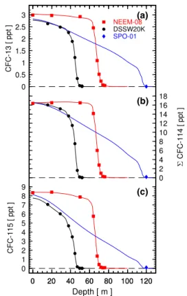
Similar to the study by Vollmer et al. (2016) for halons, the present analysis uses a firn air model to characterize the age of the CFCs in the firn air samples (Trudinger et al., 2016), the AGAGE 12-box model to relate atmospheric mole fractions to surface emissions (Rigby et al., 2013), two in-version approaches to estimate hemispheric emissions, and a Lagrangian transport model to study regional emissions of CFC-115 in northeastern Asia. NEEM-08 DSSW20K SPO-01 0 20 40 60 80 100 120 0 0.5 1 1.5 2 2.5 3 (a) CFC-13 [ ppt ] 0 20 40 60 80 100 120 Depth [ m ] 0 2 4 6 8 10 12 14 16 18 CFC-114 [ ppt ] (b) 0 1 2 3 4 5 6 7 8 9 CFC-115 [ ppt ] (c)
Figure 2. Depth profiles for the three chlorofluorocarbons CFC-13 (a), 6CFC-114 (b), and CFC-115 (c) in polar firn. Measured dry-air mole fractions are shown for the Greenland site NEEM-08 (red squares) and the Antarctic sites Law Dome (DSSW20K, black cir-cles) and South Pole (SPO-01, blue diamond). Generally the mea-surement precisions (1σ ) are smaller than the plotting symbols. The modeled mole fraction depth profiles (solid lines) correspond to the optimized emission history from the CSIRO inversion, derived from the combined observations of all three firn sites, archived air, and in situ measurements.
2.8.1 Firn model
The firn model used here was developed at CSIRO by Trudinger et al. (1997) and updated by Trudinger et al. (2013). It has previously been used for firn air measurement reconstructions of other greenhouse gases (Sturrock et al., 2002; Trudinger et al., 2002, 2016; Vollmer et al., 2016). Physical processes in the firn, foremostly vertical diffusion, cause the air samples to represent age spectra rather than an individual discrete age as is found in tank samples like the CGAA. Green’s functions are used to relate the measured mole fractions to the time range of the corresponding at-mospheric mole fractions. The update to the firn model de-scribed in Trudinger et al. (2013) included a process that had previously been neglected by Trudinger et al. (1997). This process was the upward flow of air due to compression of the pore space as new snow accumulates above, and it appears that this process is important. As discussed in Trudinger et al. (2013), including it in the model removed a discrepancy
be-Figure 3. Measurements of the chlorofluorocarbons CFC-13 (a), 6CFC-114 (b), and CFC-115 (c) from archived air samples and firn. Firn measurements are plotted against either effective or mean ages of the samples (see text). In situ measurement results from the AGAGE stations are not plotted for clarity. The inversion results are given for the Northern Hemisphere (upper solid lines) and Southern Hemisphere (lower solid lines). Growth rates (shown in orange us-ing the right axes) are globally averaged from model results. Note that zero growth, shown as dashed black lines, is offset relative to the left axes. With focus on the recent part of the record the growth rates deviate significantly from the growth rates that would be ob-tained if zero emissions were assumed (shown as maroon dashed lines, calculated by dividing the global mole fraction by the life-time).
tween DSSW20K firn and CGAA CFC-115 that was noted by Sturrock et al. (2002).
The diffusion coefficients used in this work for the three CFCs relative to CO2in air (for a temperature of 253 K) are
0.667 for CFC-13 (using Le Bas molecular volumes as de-scribed by Fuller et al., 1966), 0.495 for 6CFC-114 (Mat-sunaga et al., 1993), and 0.532 for CFC-115 (Mat(Mat-sunaga et al., 1993). Measurement results and reconstructed firn air depth profiles are shown in Fig. 2. These modeled depth profiles are not based on the observations at the individual sites but rather correspond to the optimized emission his-tory obtained using measurements from all firn sites as well as the atmospheric measurements used in this study. While 6CFC-114 was present in all samples of the three sites, CFC-13 was absent within the detection limits in the South Pole sample and in one of the deepest duplicate samples at DSSW20K. CFC-115 was also absent in two of the three deepest DSSW20K duplicate samples.
2.8.2 AGAGE 12-box model
The AGAGE box model was originally created by Cunnold et al. (1983) and has since been rewritten and modified (Cun-nold et al., 1994, 1997; Rigby et al., 2013; Vollmer et al., 2016). In the current version of the model, the atmosphere is divided into four zonal bands, separated at the Equator and at the 30◦ latitudes, thereby creating boxes of similar air masses. Boxes are also separated at altitudes represented by 500 and 200 hPa. Model transport parameters and strato-spheric photolytic loss vary seasonally and repeat interannu-ally (Rigby et al., 2013). For the CFCs analyzed here, loss in the atmosphere is dominated by photolytic destruction in the stratosphere. Here our local stratospheric loss rates are tuned to reflect the current best estimates of the global lifetimes of these compounds from SPARC (2013) as shown in Table 1.
Monthly transport parameters in the 12-box model were tuned to match the simulation of a uniformly distributed passive tracer in the Model for Ozone and Related Tracers (MOZART; Emmons et al., 2010), using Modern-Era Ret-rospective Analysis for Research and Application (MERRA) meteorology for the year 2000 (Rienecker et al., 2011). These transport parameters were repeated each year in our simula-tions. Whilst interannual variation in transport is known to impact the distribution of trace gases in the atmosphere, time-resolved atmospheric physical state estimates are not gener-ally available throughout the entire period of this investiga-tion. Furthermore, we anticipate that variations in emissions dominate atmospheric trends, particularly over the longer (multi-annual) timescales, which are our primary focus.
2.8.3 Global inversions
To estimate global emissions to the atmosphere we employ two different Bayesian inverse methods (Bristol and CSIRO). Both methods use the AGAGE 12-box model to relate ob-served tropospheric mole fractions to surface emissions of the CFCs. While past studies using the Bristol inversion have primarily targeted modern in situ observations from the AGAGE network (Rigby et al., 2011, 2014; Vollmer et al., 2011, 2015b; O’Doherty et al., 2014), the inversion method has also been extended to include firn air obser-vations (Vollmer et al., 2016). Green’s functions from the CSIRO firn model are used in both global inversions to re-late the firn air measurements to atmospheric mole fraction over the appropriate time range.
The Bristol approach is based on the methods outlined in Rigby et al. (2011) and extended in Rigby et al. (2014). Briefly, this method assumes a constraint (prior) on the rate of change of emissions, which is adjusted using the data in a Bayesian framework. The magnitude of the uncertainty in the prior yeto-year emission growth rate is somewhat ar-bitrarily chosen to be 20 % of the maximum emission rate for the entire period. In a minor modification to the approach in Rigby et al. (2014), we chose to solve for a change in
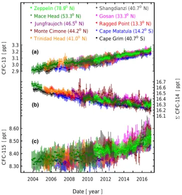
ab-Figure 4. Abundances of the chlorofluorocarbons CFC-13 (a), 6CFC-114 (b), and CFC-115 (c) at stations of the AGAGE (Ad-vanced Global Atmospheric Gases Experiment) network. These in situ data are binned into monthly means after applying a pollution filter to limit the records to samples under background conditions (O’Doherty et al., 2001; Cunnold et al., 2002). Vertical bars are standard deviations of the monthly means (1σ ). Occasional devi-ations of the Monte Cimone measurements from the other sites for 6CFC-114 and CFC-115 (CFC-13 not measured at this site) are explained by the significantly larger propagation uncertainties (par-tially caused by larger precisions) for this site compared to the other site.
solute emissions (kt yr−1), rather than use a scaling of the prior emissions. This approach was found to lead to more consistent posterior emission uncertainty estimates between the near-zero and relatively high emission periods.
The random component of the model–measurement mis-match uncertainties in the Bristol inversion is composed of measurement uncertainties and those of the atmospheric and firn air models. The atmospheric model uncertainty is as-sumed to be equal to the variability in the estimated baseline within each monthly mean. These uncertainties are propa-gated through the model to provide a posterior emission un-certainty estimate (Rigby et al., 2014). The posterior emis-sion uncertainty is then augmented with a term related to the calibration scale uncertainty and the uncertainty due to the lifetime (Rigby et al., 2014). The observations that are compared with the 12-box model in the Bristol inversion (see following section) are from all the firn air (firn model output) and CGAA archived air samples described here and the monthly mean background-filtered in situ measurements
from Mace Head, Trinidad Head, Ragged Point, Cape Matat-ula, and Cape Grim (Fig. 4).
The CSIRO inversion, also combined with the 12-box model and Green’s functions from the CSIRO firn model (Trudinger et al., 2016; Vollmer et al., 2016), was developed to focus on sparse observations from air archives and firn air and ice core samples that are associated with age spectra. The characteristics of these data necessitate the use of con-straints on the inversion to avoid unrealistic oscillations in the reconstructed mole fractions or negative values of mole frac-tion or emissions. The CSIRO inversion therefore uses non-negativity constraints and favors relatively small changes to annual emissions in adjacent years rather than large, unrealis-tic fluctuations. A prior emission history based on bottom-up estimates is used as a starting point, then a nonlinear con-strained optimization method is used to find the solution that minimizes a cost function consisting of the model–data mis-match plus the sum of the year-to-year changes in emissions (Trudinger et al., 2016). The observations used in the CSIRO inversion are the firn measurements and annual values of mole fraction from a smoothing spline fit to measurements at Cape Grim and the CGAA and another spline fit to Mace Head and the NH air archive. Uncertainties are estimated us-ing a bootstrap method that incorporates data uncertainties and uncertainties in the firn model through the use of an en-semble of firn Green’s functions.
We use the expanded AFEAS bottom-up inventory-based data for 6CFC-114 and CFC-115 as prior in the inversions as these were produced without any input from atmospheric observations. For CFC-13, emission inventories do not exist to the best of our knowledge. As prior for this compound, we use the expanded CFC-115 AFEAS data, which we scale with a factor of 1/7 based on an intercomparison of produc-tion estimates (see Supplement).
2.8.4 Regional-scale source allocation and atmospheric inversion
Pollution events of the three compounds are absent, to within detection limits, from the measurements at all AGAGE field stations with the exception of Gosan (South Korea) and Shangdianzi (China). This has prompted a more detailed analysis of these compounds in northeastern Asia to lo-cate and quantify potential sources. Only observations from Gosan were used since these are less locally influenced, and therefore less subject to sub-grid-scale model errors, than those from Shangdianzi, which are subject to pollution events originating in the nearby Beijing capital region.
We calculated qualitative emission distributions by com-bining model-derived source sensitivities with the baseline observations from Gosan above. A smooth statistical base-line fit (Ruckstuhl et al., 2012) was subtracted from the ob-servational data. Surface source sensitivities were computed with the Lagrangian particle dispersion model FLEXPART (Stohl et al., 2005) driven by operational analysis and
fore-Table 2. By-country emissions of CFC-13, 6CFC-114, and CFC-115, estimated by the regional inversion: prior and posterior estimates. Emissions from areas with HFC-125 factories are termed “hot spot”. All values are given in units of kt yr−1; uncertainties represent a 1σ range.
Compound Year China Hot spot South Korea Japan
Prior Posterior Prior Posterior Prior Posterior Prior Posterior CFC-13 2012 0.1 ± 0.045 0.14 ± 0.03 – – 0.004 ± 0.004 0.001 ± 0.002 0.01 ± 0.008 0.007 ± 0.006 CFC-13 2013 0.1 ± 0.043 0.20 ± 0.03 – – 0.004 ± 0.004 0.001 ± 0.002 0.01 ± 0.008 0.007 ± 0.005 CFC-13 2014 0.1 ± 0.043 0.15 ± 0.03 – – 0.004 ± 0.004 0.003 ± 0.002 0.01 ± 0.008 0.007 ± 0.006 CFC-13 2015 0.1 ± 0.045 0.10 ± 0.03 – – 0.004 ± 0.004 0.002 ± 0.002 0.01 ± 0.008 0.004 ± 0.006 CFC-13 2016 0.1 ± 0.045 0.10 ± 0.03 – – 0.004 ± 0.004 0.001 ± 0.002 0.01 ± 0.008 0.004 ± 0.005 [1.5ex] 6CFC-114 2012 0.4 ± 0.37 0.66 ± 0.23 – – 0.015 ± 0.033 0.007 ± 0.008 0.04 ± 0.065 0.019 ± 0.026 6CFC-114 2013 0.4 ± 0.35 1.00 ± 0.24 – – 0.015 ± 0.034 0.005 ± 0.005 0.04 ± 0.068 0.033 ± 0.029 6CFC-114 2014 0.4 ± 0.35 0.64 ± 0.21 – – 0.015 ± 0.034 0.003 ± 0.006 0.04 ± 0.067 0.017 ± 0.027 6CFC-114 2015 0.4 ± 0.37 0.61 ± 0.17 – – 0.015 ± 0.033 0.004 ± 0.007 0.04 ± 0.065 0.034 ± 0.036 6CFC-114 2016 0.4 ± 0.37 0.79 ± 0.23 – – 0.015 ± 0.033 0.003 ± 0.008 0.04 ± 0.065 0.019 ± 0.034 [1.5ex] CFC-115 2012 0.2 ± 0.68 0.25 ± 0.36 0.018 ± 0.13 0.046 ± 0.039 0.007 ± 0.051 0.004 ± 0.008 0.02 ± 0.13 0.020 ± 0.066 CFC-115 2013 0.2 ± 0.62 0.68 ± 0.25 0.018 ± 0.13 0.28 ± 0.03 0.007 ± 0.053 0.002 ± 0.005 0.02 ± 0.12 0.029 ± 0.035 CFC-115 2014 0.2 ± 0.62 0.59 ± 0.26 0.016 ± 0.13 0.18 ± 0.04 0.007 ± 0.053 0.002 ± 0.006 0.02 ± 0.12 0.048 ± 0.038 CFC-115 2015 0.2 ± 0.68 0.78 ± 0.35 0.018 ± 0.13 0.080 ± 0.041 0.007 ± 0.051 0.002 ± 0.009 0.02 ± 0.12 0.015 ± 0.032 CFC-115 2016 0.2 ± 0.62 0.47 ± 0.41 0.018 ± 0.13 0.12 ± 0.06 0.007 ± 0.053 0.005 ± 0.008 0.02 ± 0.12 0.009 ± 0.029
casts from the European Centre for Medium-Range Weather Forecasts (ECMWF) Integrated Forecasting System (IFS) modeling system. For each 3-hourly time interval 50 000 model particles were released and followed backward in time for 10 days. Surface source sensitivities (concentration foot-prints) were obtained by evaluating the residence times of the model particles along the backward trajectories (Seibert and Frank, 2004).
Qualitative emission distributions were then calculated as a spatially distributed, weighted concentration average using the source sensitivities as weights. This method is based on the one described by Stohl (1996) for simple air mass tra-jectories but was generalized for source sensitivities and pre-viously applied to halocarbon observations (Stemmler et al., 2007; Vollmer et al., 2015a). The method provides a general first impression of potential source locations but cannot be used to quantify individual sources and their uncertainty (lo-cation and length).
In addition, we applied a spatially resolved, regional-scale emission inversion using the same FLEXPART-derived source sensitivities and the Bayesian approach described in detail in Henne et al. (2016). In contrast to the method above, the Bayesian inversion provides a quantitative spatial distri-bution of posterior emissions and their uncertainties. Prior emissions were set proportional to the population density. The same emission factor per person was used for the en-tire inversion domain, which comprised most of China, North and South Korea, and the southwestern part of Japan. This emission factor was set in such a way that total Chinese emis-sions were in line with China’s share of the gross world prod-uct of approximately 15 % and the global emission estimates described in Sect. 3.2.1, 3.2.4, and 3.2.6.
Parameters describing the covariance uncertainty matrices were derived from a log-likelihood maximum search (Micha-lak et al., 2005; Henne et al., 2016). The prior emission
un-certainties obtained from this optimization were relatively large and amounted to 0.04, 0.4, and 0.6 kt yr−1 for China for CFC-13, 6CFC-114, and CFC-115, respectively (see Ta-ble 2). All analysis was performed separately for each year from 2012 to 2016. More details on the applied method and additional results can be found in the Supplement.
3 Results and discussion
3.1 Atmospheric histories and high-resolution records
We combine our measurement results from firn air samples, archived air in canisters, and in situ measurements to produce the full historic records for 13, 6114, and CFC-115 spanning nearly 8 decades (Figs. 3–4). The modeled records discussed in this section derive from the Bristol and CSIRO inversions using these observations and the AGAGE 12-box model. The firn air depth profiles show a steady de-cline of all three CFCs with increasing depth (Fig. 2). All three compounds are at or below detection limits in the deep-est samples of the Antarctic DSSW20K profile but clearly detectable in the deepest samples in the Greenland NEEM-2008 profile. These firn air results are plotted with the full historic record in Fig. 3 using dates based on the effective ages unless the mole fractions were near zero, when mean ages were used; note that these dates are used for graphi-cal purposes only and that the full Green’s functions (shown in the Supplement) were used in the inversions to represent the age of the compounds in firn air. On the temporal scale the firn air results overlap strongly with the results from the archived canisters. These canister samples span from the late 1970s to near present and overlap with the high-resolution in situ measurements shown in more detail in Fig. 4. The in situ data are binned into monthly means after applying a
Figure 5. Comparison of the atmospheric records of CFC-13 (a), 6CFC-114 (b), and CFC-115 (c) from this study with previous results. Cape Grim Air Archive (CGAA) samples and subsamples have been analyzed multiple times – here we show analysis results published by Oram (1999), Laube et al. (2016), and the present study (three separate analysis sets are averaged; see Supplement). Light grey bands denote the uncertainty on our SH model results including calibration uncertainty. Uncertainty bands for the NH, which are similar to the SH, are omitted from this plot for clarity. Results for 6CFC-114 are from combined measurements of the two analytically unseparated C2Cl2F4
isomers. Exceptions to this are the studies by Oram (1999) and Laube et al. (2016) in which the numerical sums of the two individual isomer measurements are shown. Also, results by Chen et al. (1994) (values approximated only from their graphical display) are of CFC-114 only. Assuming a 5–6 % contribution of CFC-114a in 6CFC-114, these results are still significantly lower compared to our study. All results are left on the calibration scales of the published data.
lution filter to limit the records to samples under background conditions (O’Doherty et al., 2001; Cunnold et al., 2002).
3.1.1 CFC-13
CFC-13 first appeared in the atmosphere in the late 1950s to early 1960s (Fig. 3). Its growth rates were highest in the 1980s with a significant decline thereafter, presumably as a consequence of reduced emissions due to restrictions on production and consumption by the Montreal Protocol in the non-Article 5 countries. Because of its very long lifetime, small emissions are sufficient to maintain the observed in-crease in its abundance, and consequently CFC-13 contin-ued to grow monotonically to a globally averaged mole
frac-tion of 3.18 ppt in 2016. Its global growth rate leveled off in the late 1990s but has remained at a surprisingly high mean growth rate of 0.02 ppt yr−1since 2000 with no indication of a further decline in the growth rate since then.
Cape Matatula and Cape Grim, which are the two stations most influenced by SH air masses, have shown a small and consistent offset of 0.04 ppt compared to the NH stations (SH lower), which points to predominantly NH emissions (Fig. 4). For the overlapping period of 1978–1997, our CFC-13 abundances are significantly lower (∼ 25 %) compared to earlier published data (Oram, 1999; Culbertson et al., 2004) (Fig. 5).
For most of the AGAGE field stations the high-resolution records show an absence of CFC-13 pollution events,
indicat-ing vanishindicat-ing emissions within the local footprints of these stations. However, Gosan and Shangdianzi feature sporadic pollution events with abundances that reach up to ∼ 6 ppt. Measurements from the urban sites Tacolneston (England), Dübendorf (Switzerland), and Aspendale (Australia, after re-moval of a nearby CFC-13 source in early 2010) show no pollution events, while those at La Jolla (USA) exhibit oc-casional pollution events, which, however, are smaller and less frequent than those at the two Asian field sites. High-resolution records are shown in the Supplement.
3.1.2 6CFC-114
6CFC-114 appeared in the atmosphere in the late 1950s to early 1960s at similar times to CFC-13 (Fig. 3). Its growth rate was highest in the 1970s and 1980s (0.5–0.8 ppt yr−1) and declined strongly in the 1990s. 6CFC-114 global mole fractions peaked in 1999–2002 at 16.6 ppt and have slightly declined since then to 16.3 ppt in 2016. Based on the data as-similated into the Bristol inversion framework, global growth rates have been negative since the early 2000s with a mini-mum at −0.04 ppt yr−1(mean 2004–2006) but no indication of a further decline since then. A small interhemispheric gra-dient has been persisting over the last decades as is shown by the lower mole fractions for Cape Matatula and Cape Grim compared to the NH sites (Fig. 4).
Our SH 6CFC-114 results exhibit lower mole fractions than those of Oram (1999) and those of Sturrock et al. (2002), who used a combination of the data from Oram (1999) and in situ AGAGE Cape Grim data from older instrumentation (Fig. 5). Also, our 6CFC-114 abundances are significantly lower than those of Martinerie et al. (2009) for the records before 1980. In contrast, our CGAA mole fractions agree closely with the sum of the CFC-114 and CFC-114a mole fractions from Laube et al. (2016) in the older part of the record but become progressively higher (up to 2.5 %) for the modern part of the record compared to that reported by Laube et al. (2016).
The high-resolution records at the AGAGE field sites gen-erally show no 6CFC-114 pollution events, indicating van-ishing emissions in the air mass footprints of these stations (see Supplement). The single exception is Gosan, which shows frequent pollution events reaching mole fractions of up to ∼ 20 ppt (Shangdianzi data are hampered by an instru-mental artifact and not further discussed here). The urban sites also exhibit a pattern as discussed for CFC-13 similar to Tacolneston, Dübendorf, and Aspendale featuring minor and infrequent pollution events, indicating that even in these urban areas emissions are small. However, the record at La Jolla shows very frequent pollution events with magnitudes of up to ∼ 25 ppt. This can be caused by either a rather local source or more widespread emissions in the air mass foot-print of this station. A more detailed analysis is beyond the scope of this study.
3.1.3 CFC-115
CFC-115 appeared in the atmosphere with a delay of nearly a decade compared to CFC-13 and 6CFC-114. Its growth peaked at times similar to CFC-13 and the second maximum of 6CFC-114, at rates of 0.4–0.5 ppt yr−1. Its growth then slowed during the mid-2000s to near zero, with CFC-115 abundances leveling off at ∼ 8.3 ppt in the late 1990s. How-ever, surprisingly, the CFC-115 growth rate has increased since its minimum at 0.007 ppt yr−1 (mean 2004–2009) to ∼0.026 ppt yr−1(mean 2014–2016). This has caused an en-hanced increase in the atmospheric abundances to 8.49 ppt in 2016, which is seen more clearly in the recent in situ mea-surements from the stations, with increases led by Northern Hemisphere sites (Fig. 4).
Our CFC-115 abundances agree well with earlier-published results by Culbertson et al. (2004), Oram (1999), Martinerie et al. (2009), and the younger part of the record by Sturrock et al. (2002), as is shown in Fig. 5. The latter study found somewhat larger mole fractions in the 1970s and 1980s, but this was mainly due to a process neglected in the old version of the CSIRO firn model (upward flow of air due to compression, as mentioned above). There are currently no other published data records covering the past 2 decades to which we could compare our results.
The high-resolution records at the AGAGE field sites show, similar to CFC-13 and 6CFC-114, no pollution events, with the exception of a few rare and small excursions for some of the sites. Again, Gosan and Shangdianzi exhibit pol-lution events (typically up to 13 ppt), which have become more frequent since 2013 for Gosan, and are evident in the Shangdianzi record only starting in 2016 because of missing data for 2013–2016. The urban sites La Jolla and Düben-dorf, particularly the former, exhibit pollution events with a more regular frequency. Aspendale showed CFC-115 pol-lution episodes mainly in 2006–2009 but to a much lesser degree in the most recent part of its record. CFC-115 pollu-tion events are mostly absent from Tacolneston (see Supple-ment). These observations demonstrate that CFC-115 has not completely been removed from installed equipment in these urban areas.
3.2 Emissions
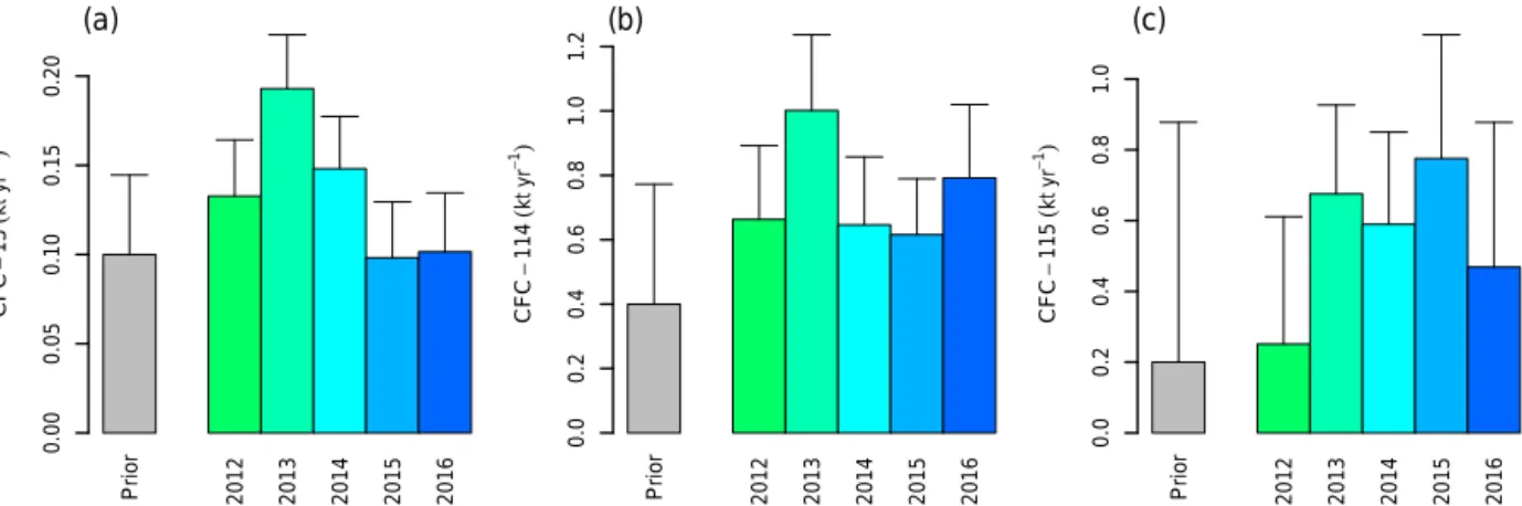
Global emissions of the three CFCs were calculated using the Bristol and CSIRO inversions covering nearly 8 decades and are shown in Fig. 6 for 1950 to 2016. For 6CFC-114 and CFC-115, industry-based bottom-up and other reported emissions are available for comparison. For all three CFCs we find persistent lingering emissions in the past decades. While the emissions for CFC-13 and CFC-114 have re-mained stable (within uncertainties), those for CFC-115 have increased in recent years. In our discussion of these recent emissions we assume that other effects that could artificially create these lingering emissions, i.e., a slowdown of vertical
Figure 6. Global emissions of the chlorofluorocarbons CFC-13 (a), 6CFC-114 (b), and CFC-115 (c) from atmospheric observations. Black lines and grey shaded areas are for the Bristol inversion and green lines and green shaded areas for the CSIRO inversion (see text). Emissions from Laube et al. (2016) are the sum of the emis-sions of both C2Cl2F4isomers. In the insets, our observation-based
global emissions and the expanded AFEAS bottom-up emissions are compared to the East Asian emissions (maroon diamonds).
air mass exchange between the troposphere and the strato-sphere and/or reduced removal fluxes, are absent. The global emission results are complemented with results for Asian re-gional emissions and with emissions found from specific pro-cesses (CFC-13) and compound impurities (CFC-115).
3.2.1 CFC-13 global emissions
Based on our inversions, CFC-13 emissions increased to a maximum of ∼2.6 ± 0.25 kt yr−1(1 SD) in the mid-1980s with a subsequent decline to relatively stable mean emis-sions of 0.48 ± 0.15 kt yr−1 during the last decade (2007– 2016, Fig. 6). Cumulative emissions until 2016 amount to 62 kt (both inversions), of which, due to its 640-year life-time (Table 1), ∼ 90 % is still in the atmosphere. The persis-tent emissions over the past 2 decades are surprisingly high (> 15 % of the peak emissions). The absence of a clear down-ward trend over this long period is inconsistent with a po-tential gradual replacement of CFC-13 in refrigeration units after the ban by the Montreal Protocol, which would lead to a decline of CFC-13 banks and emissions. Release functions
for the other two CFCs used in the AFEAS vintage model (see Supplement) indicate that emissions of the whole charge of individual refrigeration equipment after installation take 20 years for 6CFC-114 and 10 years for CFC-115. Assum-ing similar emission functions for CFC-13 in these applica-tions could potentially explain the decline in the emissions in the 1990s but not the tailing emissions thereafter, about which we can only speculate. One explanation could be dif-ferent release functions in the last 2 decades, for example a better containment for some time as a response to reduced availability of CFC-13 for refill, followed by a recent pe-riod of enhanced release perhaps due to intensified removal of old refrigeration equipment. Alternatively, CFC-13 could be emitted from sources other than refrigeration systems. It could be a by-product of fluorochemical manufacture and be released from the processes or as an impurity of the end prod-ucts. It is unlikely that CFC-13 is used as a process agent as it would need to be recorded and controlled under the regu-lations of the Montreal Protocol, which is, as far as we know, not the case. The many CFC-13 pollution events measured at Shangdianzi and Gosan, and the rare occurrence at other sites, point to emissions in the East Asian region (although emissions may also be taking place in regions not seen by our high-frequency network).
3.2.2 CFC-13 emissions from regional FLEXPART inversion
The transport analysis of CFC-13 pollution peaks that were observed at Gosan did not reveal consistent and localized sources for the years 2012 to 2016. The strongest indica-tion of sources was observed for 2013 and 2014 in China, whereas in 2015 and 2016 no specific source region could be identified (see Supplement). The Bayesian inversion showed relatively weak performance of the simulated prior time se-ries (see Supplement) and the use of the posterior emission field did not improve these simulations to a large extent, with the exception of the year 2013, for which a consider-able improvement of the simulation was achieved through the emission inversion. Consequently, the posterior emissions of CFC-13 stayed relatively close to the prior estimates, with the general tendency of lower posterior estimates for South Korea and Japan (Table 2, Fig. 7). Chinese emissions re-mained very close to the prior estimates except for the year 2013. In summary, these results do not indicate an over-proportionate share of CFC-13 emissions from northeast-ern Asia compared with the global estimate and, considering the relatively weak model performance, are connected with a considerably large uncertainty.
3.2.3 CFC-13 emissions from aluminum smelters
CFC-13 was previously found in the emissions from alu-minum plants (Harnisch, 1997; Penkett et al., 1981). Our present CFC-13 study has prompted us to reanalyze emission