Perfectly Matched Layers for time-harmonic transverse electric wave propagation in cylindrical and toroidal gyrotropic media

HAL Id: cea-02103360

https://hal-cea.archives-ouvertes.fr/cea-02103360

Submitted on 18 Apr 2019

HAL is a multi-disciplinary open access

archive for the deposit and dissemination of sci-entific research documents, whether they are pub-lished or not. The documents may come from teaching and research institutions in France or abroad, or from public or private research centers.

L’archive ouverte pluridisciplinaire HAL, est destinée au dépôt et à la diffusion de documents scientifiques de niveau recherche, publiés ou non, émanant des établissements d’enseignement et de recherche français ou étrangers, des laboratoires publics ou privés.

electric wave propagation in cylindrical and toroidal

gyrotropic media

Laurent Colas, J. Jacquot, J. Hillairet, W. Helou, W. Tierens, S. Heuraux, E.

Faudot, Lingfeng Lu, G. Urbanczyk

To cite this version:

Laurent Colas, J. Jacquot, J. Hillairet, W. Helou, W. Tierens, et al.. Perfectly Matched Layers for time-harmonic transverse electric wave propagation in cylindrical and toroidal gyrotropic media. Journal of Computational Physics, Elsevier, 2019, 389, pp.94-110. �10.1016/j.jcp.2019.02.017�. �cea-02103360�

Perfectly Matched Layers for time-harmonic transverse

electric wave propagation in cylindrical and toroidal

gyrotropic media

L. Colas1, J. Jacquot2, J. Hillairet1, W. Helou1+, W. Tierens2, S. Heuraux3, E. Faudot3, L. Lu1†, G. Urbanczyk1

1

CEA, IRFM, F-13108 Saint Paul Lez Durance, France.

2

Max-Planck-Institut für Plasmaphysik, Garching, Germany.

3

Université de Lorraine - CNRS Institut Jean Lamour F-54011 Nancy.

+

Present adress: ITER Organization, Route de Vinon sur Verdon, CS 90 046, 13067 St Paul Lez Durance, France.

† present address: TianQin Research Center for Gravitational Physics, School of Physics and Astronomy, Sun Yat-Sen University, Zhuhai 519082, P. R. China

Abstract:

In this paper we implement the stretched-coordinate Perfectly Matched Layer (PML) technique in [Texeira1998b] to emulate full power absorption outside the simulation domain for time-harmonic electromagnetic wave propagation in presence of gyrotropic dielectric tensor and curved geometry relevant for magnetized plasma devices. We recall the PML formulation as an artificial inhomogeneous lossy medium, following the stretching into the complex plane of a general system of three orthogonal curvilinear coordinates. We apply the general method in cylindrical and toroidal geometries. We then assess this technique in a simple case combining gyrotropy and coordinate curvature. Our test problem analytically quantifies the reflection of Transverse Electric (TE) cylindrical eigenmodes in a gyrotropic medium by a radial PML in cylindrical geometry. The obtained reflection coefficient involves wave, PML and geometric parameters at the PML location. The new coefficient generalizes the one obtained earlier with Cartesian coordinates, and becomes equivalent when the effects of the local cylindrical curvature at the PML (stretched) location can be neglected. These curvature effects are outlined and the limitations they impose on the properties of the PML are quantified as a function of the relevant parameters. Peculiarities related to the gyrotropy are also highlighted. Finite element calculations of the test problem in two-dimensional cylindrical geometry are exploited to verify these properties numerically. Indications are finally given on how to choose the PML parameters in order to obtain a minimal wave reflection at given numerical cost, taking into account errors associated with the numerical scheme.

I.

Introduction

This paper deals with the numerical simulation of time-harmonic electromagnetic (EM) wave propagation. In such problems the time-harmonic Maxwell’s equations in the medium are complemented with suitable boundary conditions. In finite difference or finite element calculations of EM wave propagation, Perfectly Matched Layers (PMLs) aim at emulating radiation at infinity inside a bounded simulation domain. For some applications, the EM waves are fully absorbed at finite distance from the wave launchers. But this distance is still too large to include the damping region in the simulation domain with reasonable computing resources, or the damping mechanism cannot be simulated easily. In these cases PMLs also apply, but they can be introduced at unusual locations, e.g. the inner part of the simulation domain instead of its outer boundary. This unusual setting will be met in the paper, but the results obtained also apply to more standard PMLs after minor adaptation.

In complex media such as cold magnetized plasmas, featuring a gyrotropic dielectric tensor, gyrotropy introduces two different wave propagation eigenmodes, referred to as Fast and Slow waves in the context of plasma physics [Swanson2003]. In the literature PMLs were already devised for the propagation of one eigenmode of gyrotropic media, generally in two dimensions (2D) transverse to the direction of anisotropy, and described by a scalar Helmholtz equation [Velasco2009]. This result was recently extended in 3D for the two eigenmodes, described by a vector time-harmonic wave equation [Gondarenko2004] [Jacquot2013]. Reference [Bécache2017] explored the transient EM pulse propagation in uniaxial media using the Finite Difference Time Domain (FDTD) method and PMLs adapted for each eigenmode. Reference [Jacquot2013] implemented PMLs adapted for cold magnetized plasmas at the edge of (flattened) toroidal magnetic fusion devices in the Radio-Frequency (RF) module of the COMSOL finite element solver [COMSOL]. As first proposed by [Texeira1998a] PMLs were defined as artificial inhomogeneous lossy dielectric and magnetic media, where the standard equations of electrodynamics could be applied. This was achieved by stretching the conventional Cartesian coordinates of a flattened tokamak along prescribed trajectories in the complex plane.

For many realistic applications however, using Cartesian coordinates appears to be a limitation. Flattening a toroidal tokamak is an approximation, historically intended to enable using spectral methods of EM wave simulation. The limits of this approximation have been explored both by modelling [Louche2011] [Jacquot2015] [Milanesio2017] and experiments in several frequency ranges [Bilato2004], [Ekedahl2015]. Cartesian PMLs can sometimes be kept in a curved geometry if the plasma-PML boundary remains flat. This is however not always possible, and in practice it might be inefficient: in uniaxial media for example, reference [Bécache2017] showed it necessary to stretch space along directions either parallel or perpendicular to the anisotropy. Otherwise propagative forward and backward waves might coexist, one of which cannot be damped by the PML. In view of simulating cylindrical RF plasma discharges (e.g. Capacitively coupled discharges [Faudot2015], helicon discharges [Crombé2015], [Furno2017], ion cyclotron-heated ones [Crombé2015], [Gekelman2016]), toroidal devices (tokamaks [Jacquot2015]) or even more complex geometries (stellarators) in a more realistic way, it is therefore tempting to stretch the spatial coordinates along the principal directions defined by the device geometry and/or the anisotropy of the medium.

Stretching curved coordinates reveals also useful in wave scattering problems. To reduce the computational cost, it is convenient to limit the simulation domain to the vicinity of the scattering object. The outer boundary of this domain then adopts a potentially complicated shape similar to that of the object. To cloak such boundary, so called “conformal PMLs” [Texeira2001], [Donderici2008] stretch space in a direction locally normal to the scattering surface. The “locally conformal PML” [Ozgun2007], [Smull2017] extends the

When moving from Cartesian to curved coordinates, the differential operators rot(.) and div(.) appearing in Maxwell’s equations modify their forms, due to the local curvature of the new coordinate systems [Angot1972]. To deal with these modifications, several PML reformulations have been proposed in [Texeira1998b] for a general system of three orthogonal curvilinear coordinates: (a) one with both complex stretching with original dielectric and magnetic tensors and (b) the second with real coordinates and modified (anisotropic) tensors. The latter “stretched-coordinate PML” amounts to replacing the wave propagation medium with an artificial anisotropic inhomogeneous one that can be easily implemented in standard full-wave solvers for Maxwell’s equations in the frequency-domain. In the adapted dielectric tensors and in the PML properties, not only the stretching functions but also the stretched coordinates appear, accounting for the local curvature of the coordinate system. Several Finite Difference and Finite Element implementations and analyses of the PML for isotropic media in orthogonal curvilinear coordinates can be found in references [Texeira2001], [Ozgun2007], [Donderici2008], [Smull2017].

One can anticipate that curvature effects might modify the wave-reflection properties of the PML, sometimes in an undesirable way. For example, reference [Texeira2001] showed that a conformal PML defined over a convex termination surface (as viewed from inside the computational domain) leads to dynamically unstable solutions when using the FDTD scheme. In Cartesian geometry a standard assessment of these PML properties is to quantify the reflection of propagative or evanescent plane waves in homogeneous media as a function of the relevant simulation parameters. This was done extensively in [Jacquot2013] for plane waves in gyrotropic media. Criteria of low reflection could be established for tuning the PML parameters. Limitations were also outlined when propagative forward and backward waves coexist in the PMLs, a peculiarity of anisotropic media. While plane waves are well suited for PML benchmark in Cartesian geometry, they are generally not adapted in curved coordinates, and alternative test-problems should be looked for.

The present paper aims at implementing the PML technique for time-harmonic EM wave propagation in gyrotropic media and in curved geometries relevant for magnetized plasma devices. A second goal is to assess this technique in a simple case exhibiting both non-diagonal dielectric tensor and coordinate curvature. Firstly we recall the stretched coordinate PML formulation proposed in [Texeira1998b], and apply it to cylindrical and various toroidal coordinates. Secondly, in the particular case of cylindrical geometry, we define analytical criteria for low reflection of waves by radial PMLs. We use for this purpose cylindrical waves that play in cylindrical geometry an equivalent role as plane waves in Cartesian coordinates. Cylindrical eigenmodes of gyrotropic media are recalled when the direction of anisotropy is along the axis of the cylinder. The PML reflection criteria for the Transverse Electric eigenmode involve wave, PML and geometric parameters at the PML location. The new results generalize those obtained earlier, and become equivalent when the effects of the local cylindrical curvature at the PML (stretched) location can be neglected. Curvature effects are outlined and the limitations they impose on the properties of the PML are quantified as a function of the relevant parameters. Peculiarities related to the gyrotropy are also highlighted. Finite Element calculations of the test problem in 2D cylindrical geometry are exploited to quantify these properties numerically. Indications are finally given on how to choose the PML parameters in order to obtain a minimal wave reflection at given computational cost, taking into account errors associated with the numerical scheme.

II.

PML formulation in curved coordinates as an artificial lossy dielectric

medium

Throughout this paper we consider time-harmonic EM fields oscillating in time as exp(+i

ω

0t) at pulsation

ω

0. In the 3-dimensional (3D) Euclidian space, the EM fields E and H

evolve according to Maxwell’s equations in the frequency domain

       = = + + = − = 0 div div i i 0 0 B D j D rotH B rotE ant ant

ρ

ω

ω

(II.1)

In equations (II.1) the oscillating current jant imposed on the antenna structures, as well as the oscillating antenna space charge

ρ

ant, were isolated from the self-consistent response of the medium to (E,H), incorporated in the linear local constitutive relations

D=εεεε(

ω

₀)E ; B=µµµµ(

ω

₀)H. (II.2)

Tensors εεεε(

ω

₀) and µµµµ(

ω

₀) can take very general forms. In references [Sachs1995], [Gedney1996], [Texeira1998], stretching the usual Cartesian coordinates into the complex plane was found beneficial to emulate radiating boundary conditions in a PML for problem (II.1). This section recalls the PML extension obtained in [Texeira1998b], by stretching the three principal directions defined by an orthogonal system of three curved coordinates. We focus on this method because it can be easily implemented in standard frequency-domain Maxwell’s equations solvers. Besides, for isotropic media and Cartesian coordinates, reference [Shin2012] showed that the stretched-coordinate PML results in significantly faster convergence than the alternative uniaxial PML for iterative Finite Difference Frequency Domain solvers. The formulation is subsequently applied to cylindrical and toroidal geometries.

A. Recall of PML formulation in orthogonal curved coordinates

In the 3D Euclidian space, we consider an orthogonal set of three curvilinear coordinates (u,v,w) such that ∇∇∇∇u.∇∇∇∇v=∇∇v.∇∇∇ ∇∇w=∇∇ ∇∇w.∇∇ ∇∇∇u=0 everywhere. The system is characterized locally by the elementary distance ds defined as:

(

)

2 2

(

)

2 2

(

)

2 2 2 , , , , , ,v wdu h u v wdv h u v wdw u h ds = u + v + w (II.3)

In the PML the spatial coordinates (u,v,w) are artificially stretched according to the rules

( )

= +

_∫

( )

→ u u u u u u S t dt t u 0 0 (II.4a)

( )

= +

_∫

( )

→ v v v v v v S t dt t v 0 0 (II.4b)

( )

= +

_∫

( )

→ w w w w w w S t dt t w 0 0 (II.4c) The triplet (u0, v0, w0) as well as the stretching functions (Su(u), Sv(v), Sw(w)) are arbitrary and can be chosen conveniently for the required application. In particular, the stretching can be extended to the complex plane. As for Cartesian frames it is essential that

“perpendicular to the other ones”: the stretched coordinate system remains orthogonal and a relation similar to (II.3) applies, with metric elements evaluated at stretched location, such as

hu(tu(u),tv(v),tw(w))=htu(u,v,w) (II.5) If the stretching extends to the complex plane, htu, htv and htw might become complex, whereas they should be real positive before the stretching. Stretching functions are equal to 1 in the main simulation domain, where the properties of the original medium are preserved. In the PML, on the contrary, we request that the new local EM fields (EPML, HPML) at location (u,v,w) be the solutions (E, H) of the original wave problem (II.1) evaluated at stretched location (tu(u), tv(v), tw(w)). To this end, problem (II.1) is replaced with a modified one

(

)

(

)

(

)

(

)

[

]

[

]

       = = + = − = 0 div div i , , i , , 0 0 PML PML ant PML PML PML PML µH εE j εE H rot µH E rot s ant s s s u v w u v w ρ ω ω (II.6)

where rots(.) and divs(.) denote the differential operators with respect to the stretched curved coordinates.

Let us introduce matrices ΣΣΣΣ(u,v,w) and ΛΛΛΛ(u,v,w) as

(

)

w v u w v u w v u w tw w v tv v u tu u h h S h h S h h S w v u           Σ Σ Σ =           ≡ 0 0 0 0 0 0 / 0 0 0 / 0 0 0 / , , Σ (II.7)

(

)

w v u v u u w w v w v u           Σ Σ Σ Σ Σ Σ ≡ 0 0 0 0 0 0 , , Λ (II.8)

Reference [Texeira1998b] showed that the modified EM problem (II.6) is equivalent to

(

)

(

)

(

(

)

)

(

)

(

)

(

)

(

)

(

)

[

]

( )

(

)

(

)

[

]

       = = + + = − = − − − − 0 div det div i , , i 1 1 1 0 0 PML PML ant PML PML PML 1 PML ΣH ΛµΣ Σ ΣE ΛεΣ Λj ΣE ΛεΣ ΣH rot ΣH ΛµΣ ΣE rot ant w v u ρ ω ω (II.9)

Relations (II.9) appear as the original electromagnetic problem (II.1), with the original differential operators rot(.) and div(.). However the original EM fields E(u,v,w) and H(u,v,w) were replaced respectively with the artificial EM fields (ΣΣΣΣEPML)(u,v,w) and (ΣΣΣΣHPML)(u,v,w). The original and artificial EM fields coincide inside the main simulation domain, where ΣΣΣΣ=1 (the identity tensor) and (EPML, HPML)=(E, H). Similarly the source terms

ρ

ant and jant were replaced respectively with det(ΣΣΣΣ)

ρ

ant and ΛΛΛΛjant. The original tensors εεεε and µµµµ were replaced respectively with the tensors εεεεPML≡(ΛεΛεΛεΛεΣΣΣΣ-1) and µµµµPML≡(ΛµΛµΛµΛµΣΣΣΣ-1) adapted to the stretched coordinates. Original and adapted tensors coincide in the main simulation domain, where ΣΣΣΣ=1 and ΛΛΛΛ=1. Also if tensor µµµµ is diagonal then the three matrices ΛΛΛΛ, µµµµ and ΣΣΣΣ-1 commute. For the general dielectric tensor εεεε one obtains.

w v u w v u ww u wv v wu u vw v u w vv w vu v uw w uv u w v uu           Σ Σ Σ Σ Σ Σ Σ Σ Σ Σ Σ Σ Σ Σ Σ = ≡ − / / /

ε

ε

ε

ε

ε

ε

ε

ε

ε

1 PML ΛεΣ ε (II.10)

and similarly for µµµµPML. Equation (II-9) shows that the problem can be implemented in any full-wave solver for Maxwell’s equations in the frequency-domain allowing full dielectric tensors of the type (II-10).

B. Implementation in cylindrical and toroidal geometries.

Implementation of the PML is formally similar in Cartesian and curved geometries. However the number of sub-cases is more important. For example in the case of isotropic media, one type of PML needs to be defined in Cartesian geometry, independent of the direction where waves need to be attenuated. In general 3 types of PMLs need to be defined in each direction. For anisotropic media the properties of the PML depend on both the type of coordinates and on the orientation of the direction of anisotropy. Some of these cases are investigated below. Equation (II.10) also shows that, in curved geometry, the implementation of a PML depends on its spatial location (u,v,w) via the stretched coordinates tu(u), tv(v) and

tw(w) appearing explicitly in εεεεPML. This reflects curvature effects in the new geometry.

We now treat more explicitly four concrete examples of coordinate systems of interest for magnetized plasma devices. For reference we recall the standard Cartesian set (x,y,z). One of the simplest systems exhibiting curvature is the cylindrical geometry. It is therefore useful for numerical tests, but also for simulating cylindrical plasma devices. The cylindrical coordinates (R,

ϕ

, Z) are defined as

     = = = Z z R y R x

ϕ

ϕ

sin cos (II.11)

For more realistic applications in tokamaks, we introduce a system of coordinates (r,

ϕ,θ

) associated to nested toroidal magnetic flux surfaces with concentric circular cross-sections.

[

]

[

]

     = + = + =

θ

ϕ

θ

ϕ

θ

sin sin cos cos cos 0 0 r z r R y r R x (II.12)

As a final example in axisymmetric toroidal geometry, suppose that we know a tokamak magnetic equilibrium under the form of nested shaped closed magnetic surfaces. In a poloidal cross section (plane R,Z at constant

ϕ

) these surfaces are labeled as

ψ

(R,Z)=constant, where

ψ

is a known smooth function, supposed to be monotonic from the innermost surface to the outermost one. Monotony ensures that ∇

ψ

is nowhere null in the definition domain.

In tokamak equilibria the innermost magnetic surface is reduced to a point. At this magnetic axis ∇

ψ

is ill-defined. Yet for PML implementation this magnetic axis is excluded. In this poloidal cross section we would like to define a second coordinate

θ

, such that:

- (P1)

θ

varies monotonically from 0 to 2π along each closed flux surface.

- (P2) ∇

θ

exists everywhere (except perhaps at the magnetic center, excluded from the discussion)

θ

can be seen as the generalization of the usual poloidal angle defined for concentric circular magnetic surfaces. The orthogonality condition (P3) writes

∇ . ∇ = 0 (II-13)

stating that

θ

is constant along the streamlines of ∇

ψ

. These streamlines, well-defined everywhere, intersect all the flux surfaces and do not cross one-another, except at the magnetic axis where they all converge. In equation (II-13) only the direction of ∇

ψ

matters. When

ψ

is replaced with any monotonic function of

ψ,

this direction is preserved. The streamlines therefore do not depend on the particular way to label the magnetic surfaces. Equation (II.13) therefore allows calculating

θ

on a given flux surface from its value on a neighboring flux surface. The problem is therefore completely determined once

θ

is defined on one flux surface. Besides, if property (P1) is fulfilled by the “boundary condition” then it is also verified on each flux surface. Several choices exist for defining this “boundary condition”, each of which determines a valid “generalized poloidal angle”. Some choices are however more convenient for practical use, because they lead to a more regular grid at some locations of interest. The coordinates (

ψ

,

ϕ, θ

) form a convenient system to locate the points in the shaped tokamak, using the squared elementary distance

= + + + + (II.14)

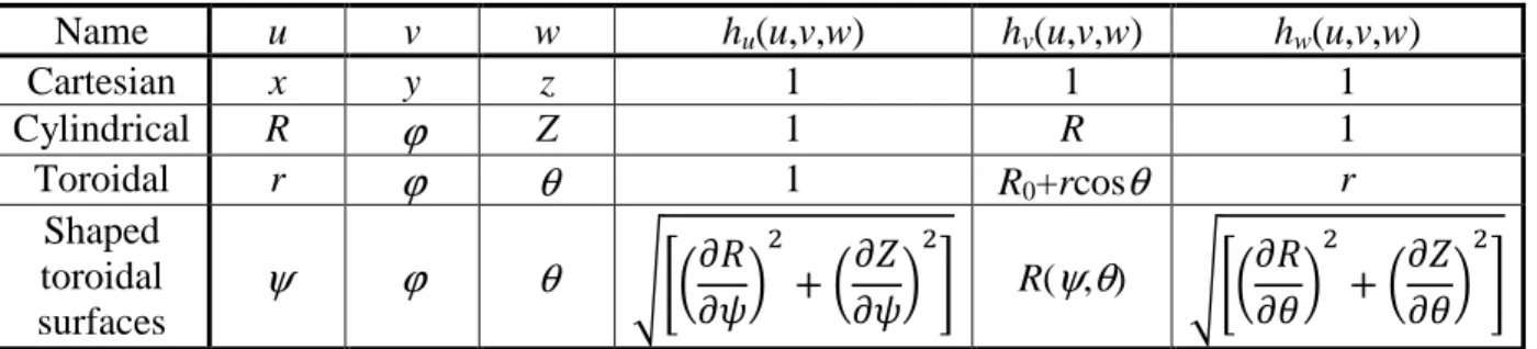
Table 1 summarizes the metric elements of the four coordinate systems. In the non-trivial cases, some of these elements can go to zero, leading to well-known singularities in the coordinate systems. Even when they lie outside the physical simulation domain, these singular points can be reached over the stretching process and therefore deserve special attention.

Name u v w hu(u,v,w) hv(u,v,w) hw(u,v,w)

Cartesian x y z 1 1 1 Cylindrical R

ϕ

Z 1 R 1 Toroidal r

ϕ

θ

1 R0+rcos

θ

r Shaped toroidal surfaces

ψ

ϕ

θ

₊ R(

ψ

,

θ

) +

Table 1: metric elements for four coordinate systems.

III.

Test problem to assess PML behaviour in cylindrical geometry.

Artificially stretching the Cartesian coordinates into the complex plane transforms propagative plane waves into evanescent ones in the PML [Sachs1995], [Gedney1996], [Texeira1998]. It therefore introduces artificial damping in this region, thus emulating radiation at infinity inside a finite simulation domain. In part II we stretched other sets of coordinates, assuming that this property might be preserved in curved geometries. However this remains to be assessed. Cylindrical geometry is a well suited test case.

A standard assessment of the PML formulation in Cartesian geometry is to quantify the reflection of propagative or evanescent plane waves in homogeneous media (see e.g. [Jacquot2013]). In cylindrical coordinates some equivalents of propagating or evanescent plane waves exist in terms of Bessel functions. In the context of plasma-filled waveguides, cylindrical eigenmodes of gyrotropic media were derived in details in [Bers1963]. These results are briefly summarized in section III.A in the case of longitudinal anisotropy. Using these tools we then propose a test problem to analytically quantify the reflection of cylindrical Transverse Electric (TE) waves by radial PMLs in cylindrical geometry, in presence of a

homogeneous gyrotropic medium. We investigate in particular how the radial curvature of the cylinder affects the PML properties compared to the Cartesian case.

A. Cylindrical eigenmodes of gyrotropic medium with longitudinal anisotropy.

From now on we seek particular solutions of the wave equations (II.1), without source term in volume, featuring a separable form in the cylindrical coordinates (R,

ϕ

, Z). The EM quantities are requested to oscillate as F(R)exp(+i

ω

0t-ikzZ-im

ϕ

), with kz a longitudinal wavevector, m (integer) an azimuthal mode number, and F(R) a radial structure function to be determined. For gyrotropic media these cylindrical waves can only be well defined when the direction of anisotropy is along Z or

ϕ

[Bers1963]. For convenience we summarize here Bers’ treatment in the homogeneous medium with longitudinal anisotropy (see also [Swanson2003]). This geometry is well suited for magnetized cylindrical plasma devices, in conditions when longitudinal invariance can be assumed. In this configuration µµµµ(

ω

0)=

µ

01 in

formula (II.2) while the dielectric tensor εεεε(

ω

0) takes the form [Swanson2003]

( )

( )

_{( )}

_{( )}

( )

( )

Z R ϕ

ω

ε

ω

ε

ω

ε

ω

ε

ω

ε

ε

ω

_        − + = _{× ⊥} × ⊥ 0 // 0 0 0 0 0 0 0 0 0 i 0 i ε (III.1)

In this configuration all the EM field components ET(R) and HT(R) transverse to Z can be expressed as a function of the longitudinal EM field components EZ(R) and HZ(R) using Maxwell-Ampère and Maxwell-Faraday equations ([Bers1963], eq. 9.21)

! = "#

$%

&⊥− ( − &_×× ⋯

−i( &⊥− (_{, #}&_× ( &_×

− _#$%_{( &× −i( &⊥− (, −i}

#$% &⊥ − &_×− (_,&_×

+i # &⊥− (_, ( &× . / / 0 _∇∇∇∇∇∇∇∇ ₂1 34× ∇∇∇∇ 1 34× ∇∇∇∇ 2 56 6 7 (III.2)

In the above expression we have introduced c=[

µ

0

ε

0]-1/2 the speed of light in vacuum,

k0≡

ω

0/c the wave-vector in vacuum, nZ≡kZ/k0 the longitudinal refractive index and

Z0=(

µ

0/

ε

0)1/2 the impedance of vacuum. In our cylindrical geometry the relevant 2D transverse

operator is ϕ R R R m _     − ∂ = ∇ / i . . T so that ϕ R R R m       ∂ = ∇ × . / i . T z

e . Substituting (III.2) into Maxwell’s equations, the two scalar fields EZ(R) and HZ(R) are then related to each other by two coupled second-order partial differential equations ([Bers1963], eq. 9.157 and 9.158)

0 2 0 =      +       ∆ Z Z Z Z T H E k H E K (III.3)

In this expression ∆_Τ. is the Laplace operator transverse to anisotropy while matrix K takes the form

8 ≡ &_{i( &}// 1 − ( /&⊥ −i #( &×/&⊥

×&/// #&⊥ &⊥− &_×/&⊥− (

Eigenmodes of the gyrotropic medium are the eigenvectors of matrix K, associated with eigenvalues n_⊥2, a squared refractive index transverse to Z. The dispersion relation for cylindrical waves writes

(

)

tr

( )

det 0

detK−n_⊥21 =n_⊥4 − K n_⊥2 + K= _(III.5)

Two separate roots n_⊥2 generally fulfil equation (III.5). Below we will investigate only media without losses in volume, for which the three dielectric constants in (III.1) are real, but without restriction of sign. In these conditions the eigenvalues n_⊥2 are also real. When

nz

ε

×/

ε

⊥=0 matrix K is diagonal and the EM fields can be explicitly split into

transverse-electric (TE) and transverse-magnetic (TM) eigenmodes with respect to direction Z

(

)

    − − = = − = = ⊥ × ⊥ ⊥ ⊥ ⊥ 2 2 22 2 2 // 11 2 / / 1 Z Z n K n n K n TE TM

ε

ε

ε

ε

ε

(III.6) In our numerical tests we will also investigate EM waves for magneto-plasmas in the Ion Cyclotron Range of Frequencies (ICRF) [Swanson2003]. Such waves satisfy the ordering |

ε

//|>>|

ε

⊥|, |

ε

×|, nZ2. A scale separation generally applies, allowing a perturbative resolution of (III.5). To leading order in the ordering the refractive indices are

(

)

[

]

(

)

(

)

    − = ≈ − − − = ≈ ⊥ ⊥ ⊥ × ⊥ ⊥ ε ε ε ε ε / 1 ) ( tr / ) /tr( ) det( 2 // 2 2 2 2 2 2 Z SW Z Z FW n n n n n K K K (III.7)

Scale separation fails close to nz2=ε⊥. Within the above ordering, the polarization of the first mode (Fast Wave or FW in ICRF) is quasi-TE.

<=,?@ A=,?@ = − BCD BCC$E⊥D_?≈ i # E=G× G//HG⊥$E₌DI (III.8)

The polarization of the alternative eigenmode (Slow Wave or SW) is to leading order A=,?@ <=,?@ = − BDC BDD$E⊥DJ≈ i E=G× KHG⊥$E₌DI (III.9)

For eigenmodes the two equations (III.3) simplify into two scalar Helmholtz equations

( )

( )

2 2 0 2 2 ; 0 _{⊥ ⊥} ⊥ = = + ∆THZ R k HZ R k k n (III.10)

and similarly for EZ(R). In our cylindrical coordinates, ∆Τ.=R-1∂RR∂R.-m2/R2 and (III.10) is a Bessel equation. When n_⊥2 is real positive, solutions of (III.10) with radiation conditions at infinity are found as Hankel functions Hm(1)(k⊥R) and Hm(2)(k⊥R) [Abramowitz]. For |k_⊥R|>>1, Hm(1)(k⊥R)~[2/(πk⊥R)]1/2exp(+ik⊥R-iπ/4-imπ/2), i.e. taking k⊥ real positive this wave behaves asymptotically as a plane wave propagating radially inwards. Similarly

Hm(2)(k⊥R)~[2/(πk⊥R)]1/2exp(-ik⊥R-iπ/4-imπ/2) propagates in the outward direction. Evanescent waves with real negative n⊥2 can be treated similarly by replacing Hm(1) and Hm(2)

with respectively the modified Bessel functions Im and Km of argument |k⊥|R [Abramowitz].

Once EZ(R) and HZ(R) are determined for each eigenmode, the transverse parts of their EM field polarizations are deduced from (III.2). Finally, the full solution of the initial EM problem (II.1) is a linear combination of the two eigenmodes determined by the source terms and boundary conditions. If a cylindrical Perfect Electric Conductor (PEC) is present at R=R1,

the two EM field components EZ(R1) and Eϕ(R1) tangent to this boundary should vanish

simultaneously. In the general case treated in [Bers1963], a mix of the two eigenmodes is needed to fulfil the PEC boundary conditions, leading to mode conversion upon wave reflection. However in the case of pure TE or TM modes, solutions exist involving only one

of the two eigenmodes. This is also approximately the case for the FW at leading order in the above ordering. For our test problem we will stick to these simple cases.

B. Reflection of propagative cylindrical TE Waves in a Radial PML.

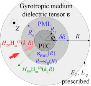
Figure 1: sketch of TE wave reflection problem to assess the radial PML.

To assess the behaviour of radial PMLs in cylindrical geometry, we study the artificial damping of an incoming propagative cylindrical TE wave in the central part of a homogeneous gyrotropic medium with longitudinal anisotropy. This situation mimics the complete absorption of a TE wave launched from the periphery of a cylindrical magnetized plasma device. The geometry of our test problem is summarized on figure 1. An incident cylindrical TE wave is launched from R→+∞ towards R=0. To attenuate artificially this incoming wave near the centre of the cylinder, a radial PML is placed in a cylindrical shell between R=R1

and R=R0=R1+

δ

R. Inside the PML the radial

coordinate R is stretched into tR(R). according to the rule

L = #+ M N_K , R1<R<R0 (III.11)

Let us assume that Im(SR(R)) adopts a given sign throughout the PML region

R1<R<R0. Due to its unusual location at the inner part of the cylinder for cloaking purposes,

Im(tR(R)) will have the opposite sign in the PML region. For a PML located in the outer part of the simulation domain, R>R0 in the PML and the two quantities would have the same signs.

The other two cylindrical coordinates (

ϕ

, Z) are not stretched. From the above calculations, and assuming here k⊥TE2>0, the radial structure of the incoming longitudinal EM magnetic field in the PML takes the form

HZiPML(R)=HZi0Hm(1)[k⊥TEtR(R)] (III.12) where the (complex) stretched radial coordinate tR(R) was substituted to the (real) radius R. The coordinate stretch preserves the TE polarization for the artificial EM electric field EPML. A PEC is placed in R=R1<R0. Alternative boundary conditions are possible there

and are briefly discussed below. For example Perfect Magnetic Conductor could be convenient for TM modes. At radius R=R1 the total tangential EM electric field should vanish.

In the case of the TE modes EZPML=0 and one should cancel only the azimuthal component

EϕPML(R1). This can be fulfilled with only incident and reflected TE waves sharing the same

(kz, m), so that the alternative eigenmode is absent from the problem. The reflected TE wave adopts a radial structure function of the form

HZrPML(R)=HZr0Hm(2)[k⊥TEtR(R)] (III.13)

E_ϕPML is obtained from HzPML using equation (III.2) with the modified operator

∇_OP = QR .

( )

[

]

(

)

( )

[

( )

]

( )

[

]

(

)

( )

[

( )

1

]

) 2 ( 1 2 1 ) 2 ( 1 ) 1 ( 1 2 1 ) 1 ( 0 0 R t k H R t k n R t k H m R t k H R t k n R t k H m H H R m R Z R m R m R Z R m theo Zi Zr ⊥ ⊥ ⊥ ⊥ × ⊥ ⊥ ⊥ ⊥ × ′ − + − ′ − + − − = =

ε

ε

ε

ε

η

(III.14)

In this expression the primes denote the derivative of the Hankel functions with respect to their arguments, and subscript TE was dropped. Equation (III.14) defines an amplitude reflection coefficient

η

theo for the TE modes, whose magnitude can be used as a figure of merit for assessing the inner PML. For a PML located in the outer part of the cylinder, the two kinds of Hankel functions would swap their roles and

η

theo should be replaced with its inverse. In the absence of coordinate stretching (tR(R)=R) the PML is replaced with an equivalent layer of gyrotropic material and |

η

theo|=1. The coordinate stretching in the PML aims at reducing |

η

theo| as much as possible.

η

theo depends on the wave characteristics (k0,nz, m), the dielectric tensor elements, the PML characteristics SR(R) as well as the PEC radial location R1. The situation is therefore

more complex than in Cartesian geometry. However only three independent non-dimensional parameters appear in formula (III.14): the complex argument k⊥tR(R1) in the Hankel functions,

the azimuthal mode number m and the ratio

ε

×/(

ε

⊥-nZ2). This latter parameter is specific of gyrotropic media. Formula (III.14) shows that this parameter introduces asymmetries in the reflection of waves with opposite m. Coordinate stretching only influences the first parameter. To shed light into the PML properties, we therefore investigate below the quantities |

η

1|=|Hm(1)[k⊥tR(R1)]/Hm(2)[k⊥tR(R1)]| and |

η

2|=|Hm‘(1)[k⊥tR(R1)]/Hm‘(2)[k⊥tR(R1)]|. They

correspond to |

η

theo| for respectively very large or very small values of m

ε

×/(

ε

⊥-nZ2). Reflection coefficient

η

1 should also replace

η

theo if [EZPML(R1)=0] and [HZPML(R1)=0] were

substituted to the PEC boundary conditions in R=R1. Reflection coefficient

η

2 would be

obtained with the boundary conditions [EZPML(R1)=0] and [∂RHZPML(R1)=0]. For increasing m,

figures 2 plot |

η

1| and |

η

2| versus the two non-dimensional real parameters (XPML, YPML) appearing in the Hankel functions:

UV_]WXY ≡ ReH"\L I

WXY ≡ ImH"\L I

(III.15)

Parameter YPML is similar to the one characterizing the efficiency of the Cartesian PML for propagating plane waves [Jacquot2013], where in this context subscript ⊥ means normal to the plasma/PML interface.

|

η

theo|=1 for YPML=0 and XPML>0. Since Hm(1)[XPML-iYPML]=Hm(2)[XPML+iYPML]* (where *

denotes complex conjugate),

η

theo is transformed into 1/

η

theo* when YPML→-YPML. Concretely this means that the PML cannot be tuned to attenuate simultaneously EM waves with real positive and real negative k⊥. As discussed in [Jacquot2013] [Bécache2017] this might be problematic in some anisotropic media where propagative forward and backward waves can coexist. Figures 2 plot only the half-plane YPML>0.

Taking YPML>0 generally reduces |

η

theo|, but not always: contrary to the equivalent Cartesian PML |

η

theo| can exceed 1 and reach very high values for positive YPML. This arises when EϕPML(R1)=0 for the reflected wave. |

η

1| reaches very high values near the complex

zeros of Hm(2), and similarly for |

η

2| near the complex zeros of H’m(2). For m=0 these zeros all

lie in the half-plane XPML<0. As m increases some zeros are progressively displaced towards

XPML>0. It is therefore important to tune Re(SR(R)) so that this zone of the complex space is avoided. Comparing the maps for |

η

1| and |

η

2| shows that the zeros can also be displaced in

a) b)

c) d)

e) f)

Figure 2: 2D Contour plots of |η1| (left panels) and |η2| (right panels) in logarithmic scale versus XPML and YPML, from formula (III.16), for increasing azimuthal mode number m. One contour line every 2.5dB. First solid

contour line corresponds to |η|=1.

Unlike the Cartesian case, the PML properties for propagative cylindrical waves depend on XPML. This parameter can be seen as a normalized radial position of the PEC boundary in the stretched coordinates. XPML can change either by moving physically the PEC radius R1 or by acting on the real part of the stretching function. The second method amounts

to artificially displacing the PEC radial position towards a region of different radius (even possibly negative!). The dependence of

η

theo on XPML can be interpreted in terms of local curvature effects at the stretched PML location.

In the limit of large |XPML+iYPML| with positive XPML one finds [Abramowitz] |Hm(1)[XPML+iYPML]/Hm(2)[XPML+iYPML]|~

|Hm’(1)[XPML+iYPML]/Hm’(2)[XPML+iYPML]|~exp(-2YPML)≡|

η

Cart| (III.16)

i.e.|

η

1|, and |

η

2|, and therefore |

η

theo| as well, converge to the same value |

η

Cart|, independent of (XPML, m) and characteristic of Cartesian PMLs [Jacquot2013]. However the minimal YPML to reach this asymptotic regime depends on (XPML, m): the higher m and the lower XPML, the higher YPML should be. In the Cartesian case, references [Bermudez2007], [Cimpeanu2015] highlighted the merits of unbounded stretching functions such that the imaginary part of YPML reaches infinity. In this case |

η

Cart| is expected to be 0 and the only residual wave reflection is that introduced by the numerical scheme for solving (II.9). Formula (III.16) shows that this favourable property is preserved in cylindrical coordinates.

The parametric region around XPML+iYPML=0 appears unfavourable for low wave reflection by the PML. At fixed PML extension

δ

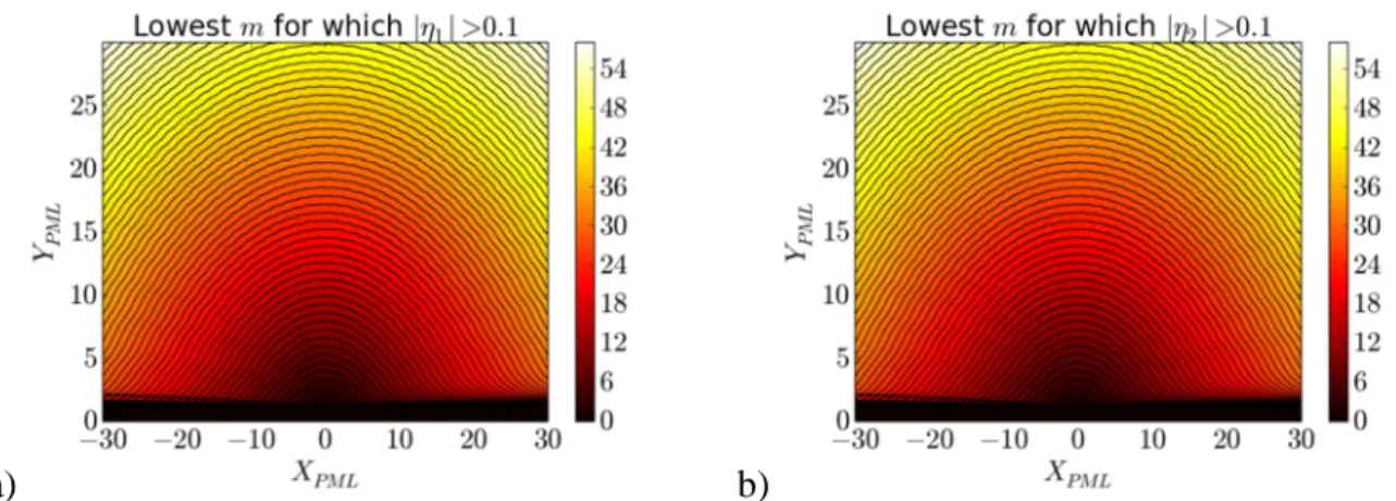
R, low values of XPML and YPML are reached for low k_⊥, i.e. for waves propagating nearly parallel to the plasma/PML interface, similar to the Cartesian case [Jacquot2013]. The size of the unfavourable region gets larger as m increases: for given (XPML,YPML), a critical value of m always exists above which the PML loses efficiency. Figures 3 map as a function of (XPML,YPML) the lowest value of m for which the amplitude ratio exceeds 0.1. In figures 3 this value is m=0 for YPML<1.2. The critical m value increases with both XPML and YPML. It can therefore be made arbitrarily high by proper PML tuning. In practical applications, only a finite number of azimuthal harmonics need to be resolved. The PML can always be tuned so that it remains efficient up to this maximum m. In particular stretching the real part of R can be beneficial if it moves artificially the PEC location towards regions of lower curvature. Larger coordinate stretching however produces larger radial variations of εεεεPML(R) and therefore can impose a finer discretization of the PML region.

a) b)

Figure 3: Lowest value of azimuthal mode number m for which the amplitude ratios exceeds 0.1, versus (XPML,YPML). a) |η1|>0.1, b) |η2|>0.1.

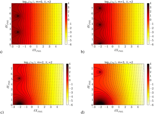
C. Reflection of evanescent cylindrical waves in a radial PML.

When k_⊥2 is real negative for the TE mode, a similar analysis as before can be made for waves that are evanescent inwards, i.e. waves growing radially as exp(+|k_⊥|R) for large R. In formula (III.14) the Hankel functions Hm(1) and Hm(2) should be respectively replaced with

the modified Bessel functions Im and Km [Abramowitz]. In the absence of coordinate

stretching, the equivalent of

η

1 writes Km(X1)/Im(X1), where X1=|k⊥|R1 is a real normalized

radius at PEC location. After the stretching, argument X1 should be transformed into

X1+

δ

XPML+i

δ

YPML where

U`VWXY<sub>`]</sub>≡ |"\|bRe L #' % c

WXY ≡ |"\|ImHL I (III.17)

Figures 4 therefore plot the ratio

|

η

3|=|Km(X1+

δ

XPML+i

δ

YPML)/Im(X1+

δ

XPML+i

δ

YPML)|*Im(X1)/Km(X1) versus (

δ

XPML,

δ

YPML). Only positive

δ

YPML are shown since negative

δ

YPML produce a similar result. |

η

3| is 1 for

(

δ

XPML,

δ

YPML)=(0,0) and should be ideally as low as possible. For given

δ

YPML,

δ

XPML>0 is always beneficial for attenuating the reflected wave compared to

δ

XPML=0, while

δ

XPML<0 might be very detrimental, especially close to

δ

XPML=-X1. For positive

δ

XPML, adding

δ

YPML is generally beneficial but not always. For large positive X, |Km(X+iY)/Im

a) b)

c) d)

Figure 4: 2D contour plots of amplitude ratio |η3| (in logarithmic scale) versus (δXPML,δYPML) from (III.18) for X1=2.0 and for the first four values of azimuthal mode number m. One contour line every 2.5dB. First solid

contour line corresponds to |η₃|=1.

IV.

Numerical tests of radial PML with gyrotropic media using 2D finite

elements.

The test problem for propagative cylindrical TE waves proposed in part III was implemented with finite elements in two dimensions (2D), and the wave reflection was quantified from the simulation output. This allows assessing numerically the analytical figure of merit

η

theo from (III-14). Simulations also illustrate specific features and limitations of the PML in cylindrical geometry. We finally investigate enhanced PML reflection associated with the finite element discretization of the simulation domain. We outline how to choose the PML parameters in order to obtain a minimal PML reflection at given numerical cost, taking into account the discretization.

A. Simulation and post-processing protocols

Using the COMSOL finite element solver [COMSOL], the test problem was simulated numerically in the 2D (radial, azimuthal) geometry (R,

ϕ

) sketched on figure 1, with EM fields assumed to vary as exp(-ikzZ) in the out-of-plane longitudinal direction Z. COMSOL includes a built-in module to simulate the standard EM problem (II.1) with standard boundary conditions and any user-defined material of type (II.2), possibly inhomogeneous in space. All over the main simulation domain, the homogeneous gyrotropic dielectric tensor (III.1) was applied. A PML was implemented in the inner part of the simulation domain. When not

precised, the artificial inhomogeneous tensors εεεεPML(R) and µµµµPML(R) from (II.10) were applied there, where εεεε is still from (III.1).

Although this choice is non-restrictive, we performed most of our numerical tests using polynomial stretching functions, for easier comparison with earlier work in Cartesian coordinates [Jacquot2013]. Specifically

SR(R)=1-(S’+iS’’)[|R0-R|/

δ

R]p, R1<R<R0 (IV.1)

From this one can define tR(R) explicitly as

( )

R R R R p S S R R t R p R

δ

δ

1 0 1 i +       − + ′′ + ′ + = → , R1<R<R0 (IV.2)

. From table 1, matrix ΣΣΣΣ(R) in formula (II.7) takes the following form

ΣΣΣΣ(R)=d N 0 0 0 L / 0 0 0 1e T (IV.3)

It differs from a Cartesian-like PML formulation by a non-trivial term

Σ

_ϕ(R)=tR(R)/R in the azimuthal direction. The PML medium features complex dielectric tensor elements, introducing artificial losses in PML volume. Besides, the three diagonal elements of εεεεPML(R) are different from each other and µµµµPML(R) becomes non-trivial. A PEC was implemented at the inner radial boundary of the simulation domain. From equation (II.9) this boundary condition applies to the EM field ΣΣΣΣEPML computed in the PML. Since matrix ΣΣΣΣ(R) is diagonal in (IV.3), this amounts to cancelling both E_ϕPML(R1,

ϕ

) and EZPML(R1,

ϕ

) all over the inner

radial boundary.

Several simulation series, summarized in table 2, scanned the plasma and PML parameters identified as important in section III. Only cases with propagative cylindrical waves were envisaged. The cases considered also feature

ε

×=0 or highly negative

ε

//, so that

the EM problem (II.10) involves only (or mainly) the TE mode. TE wave polarization is exact for all series except #12 and #14 highlighted in grey, where it is approximate since kz

ε

×≠ 0.

Consistent with this assumption the longitudinal EM electric field EZ was imposed null at the outer boundary of the simulation domain, except on series #12 and #14, where the approximate formula (III.8) was used for the FW polarization. The prescribed azimuthal EM electric field at this location was E_ϕ(R,

ϕ

)=E0exp(-im

ϕ

) to select the proper azimuthal mode

number. The outer boundary of the simulation domain was always located 1 m outside the PML outer radius. For the sake of comparison, series #1 of table 2 was also repeated using a Cartesian-like PML formulation, where

Σ

_ϕ(R)=1 was imposed in (IV.3), i.e. the effect of the cylindrical curvature was artificially suppressed.

As a first step the numerical tests tried to reproduce the analytical expectations from formula (II.14) as accurately as possible, without caring about their numerical cost. Both the main simulation domain and the PML were discretized using an unstructured mesh of quadratic Nedelec-type triangular finite elements, with typical size 1cm. The main simulation domain and the PML were meshed separately: no triangle does cross the interface between them. In simulation series #1, one finds 15 triangles over the length 1/k⊥. Up to 843474 elements were necessary to mesh the largest simulation domains, corresponding to 5908342 degrees of freedom. Calculations relied on the direct solver MUMPS.

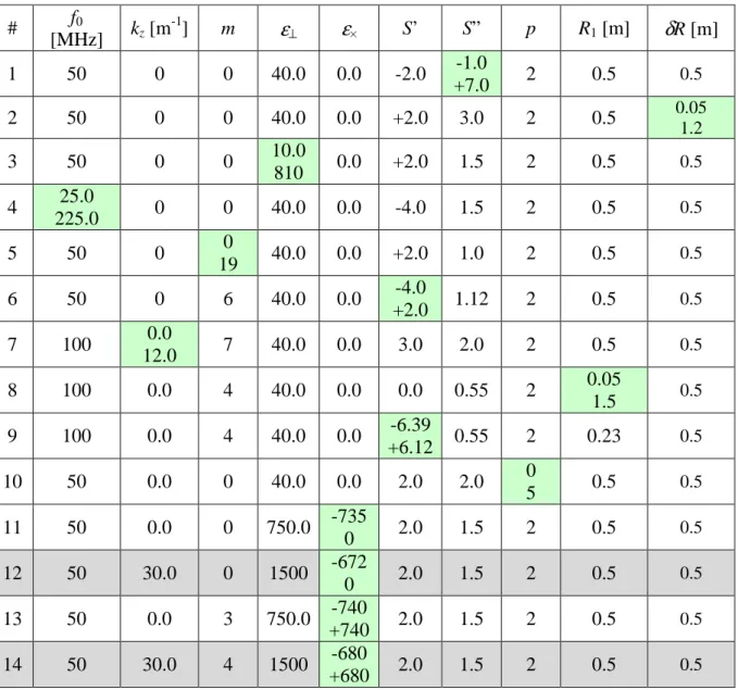
# f0 [MHz] kz [m -1 ] m

ε

_⊥

ε

× S’ S” p R1 [m]

δ

R [m] 1 50 0 0 40.0 0.0 -2.0 -1.0 +7.0 2 0.5 0.5 2 50 0 0 40.0 0.0 +2.0 3.0 2 0.5 0.05 1.2 3 50 0 0 10.0 810 0.0 +2.0 1.5 2 0.5 0.5 4 25.0 225.0 0 0 40.0 0.0 -4.0 1.5 2 0.5 0.5 5 50 0 0 19 40.0 0.0 +2.0 1.0 2 0.5 0.5 6 50 0 6 40.0 0.0 -4.0 +2.0 1.12 2 0.5 0.5 7 100 0.0 12.0 7 40.0 0.0 3.0 2.0 2 0.5 0.5 8 100 0.0 4 40.0 0.0 0.0 0.55 2 0.05 1.5 0.5 9 100 0.0 4 40.0 0.0 -6.39 +6.12 0.55 2 0.23 0.5 10 50 0.0 0 40.0 0.0 2.0 2.0 0 5 0.5 0.5 11 50 0.0 0 750.0 -735 0 2.0 1.5 2 0.5 0.5 12 50 30.0 0 1500 -672 0 2.0 1.5 2 0.5 0.5 13 50 0.0 3 750.0 -740 +740 2.0 1.5 2 0.5 0.5 14 50 30.0 4 1500 -680 +680 2.0 1.5 2 0.5 0.5

Table 2: Overview of parametric space explored over the simulations. Scanned parameters are highlighted in green. In series 1-11, ε//=-105 was used but should not play any role. In simulation series #12 and #14 highlighted in grey the TE polarization is only approximate. Series 12 was performed using ε//=-106 and ε//

=-107. Series 13 and 14 were performed with ε//=-106 and ε//=-108.

In order to numerically assess the reflection of propagating cylindrical waves by the PML, the azimuthal average of HZ(R,

ϕ

)exp(im

ϕ

) was evaluated numerically from the 2D simulation output using the FEM matrices. The

ϕ

-averaged 1D results were then sampled every millimeter in R over the main simulation domain. This corresponds to 1000 radial points, with a spatial resolution ~10 times finer than the typical finite element size. In simulation series #1, one finds 150 points over the length 1/k⊥. Using a least-square minimization procedure, the radial variation of this quantity over the main simulation domain was fitted with a linear combination of Hm(1)(k⊥R) and Hm(2)(k⊥R), with respective complex

weights HZi0_sim and HZr0_sim. In the argument of the Hankel functions, dispersion relations (III.6) or (III.7) were used to determine k_⊥ from the input parameters. Finally the magnitude of the simulated amplitude ratio

η

sim=HZr0_sim/HZi0_sim served as a figure of merit to quantify the PML reflection in the numerical tests. The fitting procedure implicitly assumes that only the TE mode with correct m is present in the simulation. In practice numerical noise is always superimposed to the ideal results, as well as the other eigenmode of the gyrotropic medium, especially in the cases where the TE polarization is only an approached input. Besides,

dispersion relation (III.7) is only approximate. All this introduces uncertainties in the numerical determination of

η

sim.

B. Comparison with analytical figure of merit.

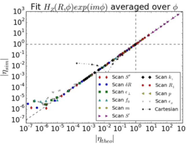
Over the simulation database, Figures 5 compare the numerical reflection coefficient

η

sim with theoretical expectation

η

theo from formula (III.14). Direct comparison of |

η

sim| with figures 2 is only possible for the simulations series #1-#12 with m

ε

×=0. Quantity

η

2 should be

used for this comparison. An important restriction to the allowed parametric space will be discussed on Figure 6 and is excluded here. |

η

sim| values well above 1 could be reached, indicating that the reflected wave can be amplified by the PML instead of being attenuated. This situation is met when the imaginary part S” of the stretching is negative, like in the Cartesian case. For positive S”, this might also be the case for some values of XPML in formula (III.15), a peculiarity of the cylindrical geometry producing the peaks on figures 2.

η

sim agrees well with

η

theo over eight orders of magnitude down to reflection levels of 2×10-6, when the precision of the simulation gets limited by either the mesh size or the fitting procedure (see section IV-D). The relative difference between

η

sim and

η

theo roughly scales as 1/min(|

η

theo|, |

η

theo|−1). This relative difference is significantly enhanced in simulation series #12 and #14 with kz

ε

×≠ 0. We speculate this is not due to the PML but because we used

approximated boundary conditions for the quasi-TE polarization: while the simulation points with

ε

//=-107 or

ε

//=-108 appear in the ballpark of the other series on figure 5.b, the runs with

ε

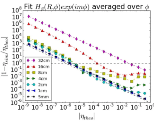
//=-106 are well above.

Figure 5.a): numerical amplitude reflection coefficient |ηsim| versus theoretical value |ηtheo| expected from formula (III.14), over simulation series #1-#14 from

table 2. Last series: same as series #1, using a Cartesian PML-like PML formulation,with Σϕ(R)=1

artificially imposed in formula (IV.3)

Figure 5.b): Same database as figure 5.a, relative difference |1-ηsim/ηtheo|, vs |ηtheo| from formula (III.14).

Tilted curves: y=10-6/x and y=10-6x

Figures 5 also show a repeat of series #1 in table 2, using a Cartesian-like formulation of the PML. In this series |

η

sim|=1 for S”=0, as it should for energetic reasons. For some values of S”, the Cartesian-like PML behaves better than the cylindrical one. This is however observed over a limited window in parametric space, and it is hardly predictable in advance. For large S”, the simulated amplitude reflection coefficient reaches an asymptotic value above 10-2, while the cylindrical PML achieves |

η

sim|<10-5. This illustrates the merits of the new PML formulation in curved coordinates.

C. Peculiarities of the cylindrical PML

Figures 6 to 8 illustrate specific properties of the cylindrical geometry that have hardly any equivalent with Cartesian coordinates.

Figure 6: Simulated amplitude reflection coefficient |ηsim| vs Re(tR(R1)). Numerical scan of R1 with S’=0, scan of S’ with R1=0.23m and predictions |ηtheo| from

formula (III.14). Horizontal dashed line: amplitude reflection coefficient|ηCart| from formula (III.14).

Simulation series #8 and #9 from table 2.

Figure 6 shows a scan of the radial position R1 for the inner PEC boundary of

the simulation domain, with S’=0. Unlike expression |

η

Cart| from (III.16), the cylindrical reflection coefficient |

η

theo| from (III.14) depends on R1. For given simulation

parameters, a minimum value of R1 exists

below which the PML becomes inefficient. The variation of |

η

sim| with R1 is

non-monotonic. This corresponds to the crossing of peaks in the 2D diagrams on Figures 2. The maximal value of the reflection coefficient can exceed 1. For large R1 the

cylindrical curvature decreases at the PML location and |

η

sim| reaches an asymptotic

value corresponding to |

η

Cart|.

Figure 6 also shows that an effect similar to the change of R1 is obtained by

stretching the real part of R, through a scan of S’ at fixed R1. From formula (III.15) the

relevant parameter to plot the results is Re(tR(R1))=R1+S’

δ

R/(p+1). Negative values of this

parameter can be reached, while R1 remains positive. However Figure 6 shows that in these

cases the PML fails to attenuate the incoming cylindrical wave, even when formula (III.14) predicts low |

η

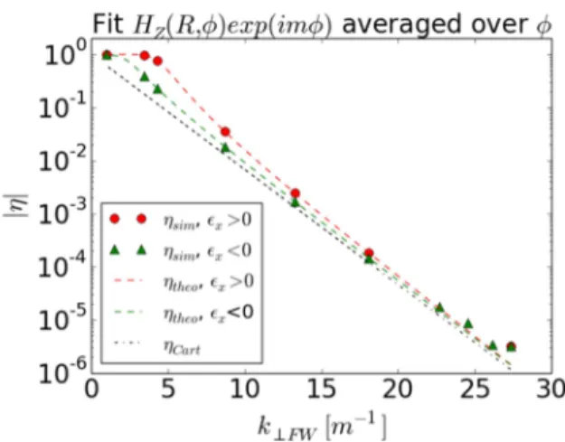
theo|. This behavior persists when the mesh is refined and cannot be ascribed to the discretization of problem (II.9). It may be linked with the crossing of a singular point of the coordinate system inside the PML. One should therefore avoid this parametric domain. The related simulation points were deliberately excluded from Figures 5.

Figure 7: reflection coefficient over a scan of ε×, vs normal wavevector k⊥,FW from equation (III.8). Data points with positive and negative ε× are plotted with different symbols. Also shown are expressions |ηtheo| from formula (III.14) and |ηCart| from formula (III.16).

Series #14 from table 2 with ε//=-108

Figure 7 plots the simulated reflection coefficients versus wavevector

k_⊥FW from dispersion relation (III.8), over a scan of

ε

× with m≠0 (series #14 of Table 2).

As for plane waves in Cartesian coordinates, low levels of reflection are observed for large k⊥FW while the PML loses efficiency for cylindrical waves propagating nearly parallel to the plasma/PML interface. However when m≠0 cylindrical waves with positive and negative

ε

× exhibit different

|

η

sim| despite equal k⊥FW. In the electrodynamics of magnetized plasmas, changing the sign of

ε

× amounts to reversing

the magnetic field direction. |

η

sim| values can differ by a factor of more than two. This peculiarity of gyrotropic media in cylindrical geometry was anticipated from

formula (III.14), and illustrates the role of parameter

ε

_×/(

ε

_⊥-nZ2). Largest ratios are obtained for medium values of k⊥FW. For low k⊥FW, |

η

sim| becomes 1 whatsoever. For large k⊥FW the reflection coefficients converge to |

η

Cart| from formula (III.16) that does not depend on the sign of

ε

×. In all cases |

η

theo| is larger than |

η

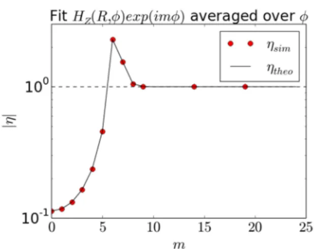
Cart|.

Figure 8: Numerical reflection coefficient ηsim, and prediction ηtheo from formula (III-14) vs azimuthal mode

number m. Simulation series #5 from table 2.

Figure 8 shows a scan of the azimuthal mode number m. Good agreement of |

η

sim| is

found with |

η

theo| from formula (III.14). The

variation of |

η

sim| with m is non-monotonic.

This corresponds to the crossing of peaks in the 2D diagrams on Figures 2. The maximal value of the reflection coefficient can exceed 1. For large m, |

η

sim| reaches an asymptotic

value of 1. A critical value of m is evidenced, above which the PML becomes inefficient.

D. Effect of finite element discretization and indications for PML tuning.

Formula (III.14) is valid in the continuous limit when the typical finite element size tends to zero. Yet a numerical computation always discretizes the simulation domain, which is expected to degrade the PML properties. The memory requirements and computation time of a 2D finite element simulation scale roughly as the inversed square of the typical element size. One therefore needs to find a compromise between these constraints and our initial request to keep the wave reflection low enough to play negligible role on the simulated phenomena. Using the simulation parameters of series #1 in table 2, this section investigates numerically the effect of finite element discretization on our test problem and provides some indications on how to find this compromise.

Figure 9.a plots |

η

sim| versus YPML over a scan of S’’ similar to series #1 for various finite element sizes in the PML. Figure 9.b is similar to figure 5.b for the scans figure 9.a. The element size in the main simulation domain was kept at 5mm. For the simulation parameters of series #1, k_⊥= 6.63m-1, i.e. in the main simulation domain one finds 30 elements over the length 1/k_⊥=15.1cm. For low values of S’’, |

η

sim| decreases with increasing YPML, following the expectations from formula (III.14). Then |

η

sim| reaches a minimal value above |

η

theo|, and

subsequently increases. As the mesh gets coarser, the saturation occurs for lower values of

S’’, and the minimal value of |

η

sim| gets larger. Therefore we attribute the saturation to the

discretization of the PML domain. Strangely enough the results slightly degrade when the mesh size in the PML is refined from 1 cm to 5 mm. We have probably reached limits due to either the discretization of the main domain or to the least-square fitting procedure to determine |

η

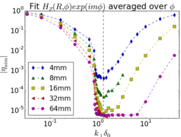
sim|. 2×10-6 is the lowest amplitude reflection coefficient that can be reliably

Figure 9.a: Numerical reflection coefficient ηsim, vs YPML from formula (III.15), over a scan of S’’ with the

parameters of series #1 in table 2, for several finite element sizes in the PML. Element size 5mm in main

simulation domain. Colored dash-dotted lines: ηsim, obtained with unbounded stretching function (IV.4),

k⊥δ0=1.5 and similar mesh.

Figure 9.b: Same database as figure 9.a, relative difference |1-ηsim/ηtheo| vs |ηtheo| from formula (III.14).

Tilted curve: y=10-6/x

For a given computational cost, figure 9.a shows an ‘optimal’ value of S’’ such that the PML reflection is minimal in presence of discretization. Either this reflection is considered low enough or one should reduce it by refining the mesh, at the expense of larger computational cost. This optimization procedure, similar to the Cartesian case, is however non-exhaustive: one could also play with the order p in formula (IV.1) or optimize all the coefficients in a polynomial expression of S(R). For the FDTD scheme in Cartesian coordinates, an example of more complete optimization was given in [Collino1998], as a function of the number of points over the PML depth and the number of points per wavelength. In the cylindrical case the PML reflection depends also on the stretched PML location (PML radius, real part of stretching function, PML depth) and the boundary conditions that can be tuned in many ways and also affect the numerical cost. When one looks for low reflection coefficients, formula (III.16) suggests that the PML behavior should be comparable to the Cartesian case in the continuous limit. But it tells nothing about discretization effects. Finally, for a realistic simulation, optimization should be undertaken not for one single cylindrical wave but for a relevant spectrum (i.e. many kz and m simultaneously, see below, and possibly several wave polarizations). We therefore expect that the optimization outcome should be quite model-dependent.

Formula (III.16) suggested the merits of unbounded stretching functions such that

YPML reaches infinity and |

η

sim| is only limited by the numerical scheme. Following

[Bermudez2007] and [Cimpeanu2015], we test below stretching functions of the form

N 1 ' fgK

$ C ; R1<R<R0 (IV.4)

Where length

δ

0 is a tunable parameter. This is not the only possible choice but it is

considered as “optimal” in Cartesian geometry [Cimpeanu2015]. The associated stretched radius is

L i`#log g_{$ C} ; R1<R<R0 (IV.5)

Over a scan of

δ

0 figure 10 plots |

η

sim| versus k⊥

δ

0 for various PML depths

δ

R and