Laboratory Experiments of Ice Scour Processes: Buoyant Ice Model

(1)

Publisher’s version / Version de l'éditeur: PERD/CHC Report 31-29, 2002-05

READ THESE TERMS AND CONDITIONS CAREFULLY BEFORE USING THIS WEBSITE.

https://nrc-publications.canada.ca/eng/copyright

Vous avez des questions? Nous pouvons vous aider. Pour communiquer directement avec un auteur, consultez la

première page de la revue dans laquelle son article a été publié afin de trouver ses coordonnées. Si vous n’arrivez pas à les repérer, communiquez avec nous à PublicationsArchive-ArchivesPublications@nrc-cnrc.gc.ca.

Questions? Contact the NRC Publications Archive team at

PublicationsArchive-ArchivesPublications@nrc-cnrc.gc.ca. If you wish to email the authors directly, please see the first page of the publication for their contact information.

Archives des publications du CNRC

For the publisher’s version, please access the DOI link below./ Pour consulter la version de l’éditeur, utilisez le lien DOI ci-dessous.

https://doi.org/10.4224/12328809

Access and use of this website and the material on it are subject to the Terms and Conditions set forth at

Laboratory Experiments of Ice Scour Processes: Buoyant Ice Model

Barker, Anne; Timco, Garry

https://publications-cnrc.canada.ca/fra/droits

L’accès à ce site Web et l’utilisation de son contenu sont assujettis aux conditions présentées dans le site LISEZ CES CONDITIONS ATTENTIVEMENT AVANT D’UTILISER CE SITE WEB.

NRC Publications Record / Notice d'Archives des publications de CNRC: https://nrc-publications.canada.ca/eng/view/object/?id=4813020e-b8ef-4a82-afa6-64e733ab6ba4 https://publications-cnrc.canada.ca/fra/voir/objet/?id=4813020e-b8ef-4a82-afa6-64e733ab6ba4

(2)

LABORATORY EXPERIMENTS OF ICE SCOUR PROCESSES:

BUOYANT ICE MODEL

Anne Barker and Garry Timco Canadian Hydraulics Centre National Research Council of Canada

Ottawa, Ont. K1A 0R6 Canada

Technical Report CHC-TR-006

PERD/CHC Report 31-29

(3)

(4)

ABSTRACT

A laboratory program was carried out to measure the loads and seabed response due to a buoyant ice block scouring a representative seabed. The results complement previous experimental data carried out at the Canadian Hydraulics Centre, which used a rigidly affixed ice block to scour seabed material representative of the Grand Banks region. The present study used the same seabed material; however in this test series, the model was towed along an ice tank, free to move throughout the water column. Seven tests were carried out. Freshwater ice, built up into a large block with an overall dimension of 0.76m x 0.76m x 0.71m, was used to scour the seabed at depths up to 0.2m. The scouring loads, displacement and angular movements and resulting trenches were measured. This report provides a description of the test arrangement and the experimental results.

(5)

(6)

3.3 Test Scour2_002 ...17 3.4 Test Scour2_003 ...20 3.5 Test Scour2_004 ...21 3.6 Test Scour2_005 ...21 3.7 Test Scour2_006 ...21 3.8 Test Scour2_007 ...21 4. ANALYSIS...23 4.1 Observational Data ...23 4.2 Scour Profiles ...24 4.3 Force Data ...26 4.4 MOTAN Data ...28 5. FINAL COMMENTS ...29 6. ACKNOWLEDGEMENTS ...30 7. REFERENCES...31 APPENDIX ... A-1

(7)

TABLE OF FIGURES

Figure 1 Photo of typical Grand Banks sand and gravel seabed (Sonnichsen,

2001)...3

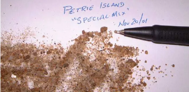
Figure 2 Sand chosen to represent Hibernia Sand Formation/Adolphus Sand (Davies, 2002)...4

Figure 3 Gravel chosen to represent the Hibernia Gravel Formation (Davies, 2002)...4

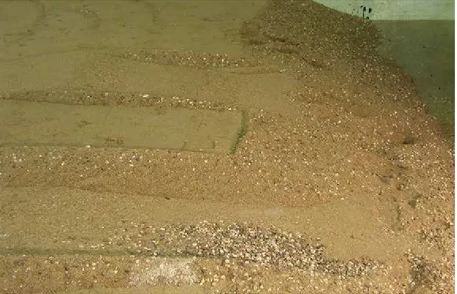
Figure 4 Photo showing the sand and gravel mixed seabed, after two tests. ...5

Figure 5 Freezing ice in mould...6

Figure 6 Front of model, with plywood bottom removed ...7

Figure 7 Back of model, with plywood bottom removed ...7

Figure 8 Photograph showing the connection between the ice block and the main carriage. ...8

Figure 9 Dynamometer mounted on main carriage, with the steel bracket that was used to support the chain ...9

Figure 10 Sketch of MOTAN set-up with respect to ice block...10

Figure 11 MOTAN mounted onto model ...10

Figure 12 Sketch of test set-up ...11

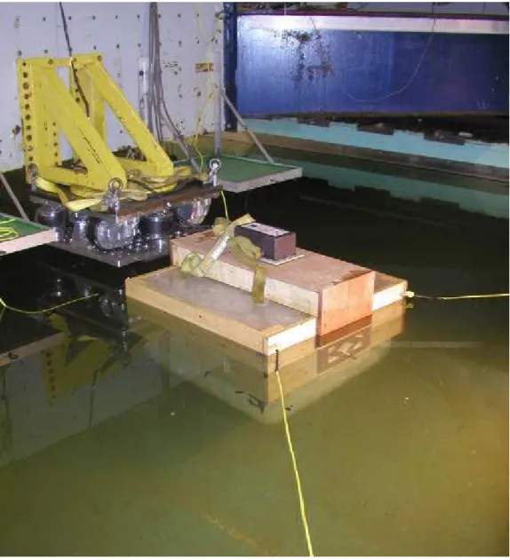
Figure 13 Test set-up showing the floating ice block with the MOTAN mounted on top. During a test, the ice block was towed approximately 1 m behind the dynamomter. ...12

Figure 14 Plot showing the free-vibration decay of the model. The “best fit” to the data indicated a natural frequency of 0.34 Hz and a damping coefficient of 1%...15

Figure 15 Photo of Scour2_002 profile. The ice block travelled from the top left of the photograph to the bottom right...16

Figure 16 Photograph a) shows the amount of freeboard immediately before the ice block begins to scour during test Scour2_002, roughly 6 cm to the top of the ice. Photograph b) shows the freeboard associated with the ice block as it slides along the surface of the seabed, now twice the initial freeboard. ...17

Figure 17 Sum of forces in the x-direction for test Scour2_002 ...18

Figure 18 MOTAN angle results for test Scour2_002 ...19

Figure 19 MOTAN motion results for test Scour2_002 ...20

Figure 20 Photo of Scour2_003 profile ...21

Figure 21 Side view of Scour2_007 profile. The direction of motion of the iceberg was from left to right in the photograph...22

Figure 22 Photo showing the chattering effect after the ice model rode up on top of the seabed material. ...23

Figure 23 Scour2_002 and Scour2_003 ...24

Figure 24 Average scour profiles ...25

Figure 25 Maximum and 98% peak forces for scour section ...27

(8)

LABORATORY EXPERIMENTS OF ICE SCOUR PROCESSES:

BUOYANT ICE MODEL

1. INTRODUCTION

The presence of icebergs is one of the main challenges facing the full development of the petroleum resources in the Grand Banks regions of Canada. In addition to being a threat to fixed (GBS) and floating (FPSO) structures, they also have a profound influence on seabed facilities and pipeline transportation systems for offshore natural gas. Icebergs have been observed to interact with the sea floor creating scour features. The nature, depth, width and zone of influence of these scours are the major factors affecting feasibility of sub-sea facilities and seabed pipelines. Although there is knowledge of the depth of existing scours (Sonnichsen and King, 2001), there is limited knowledge of the factors that control the depth and the loads associated with the scouring process.

To understand better the processes and loads of iceberg scouring, a test program was carried out at the Canadian Hydraulics Centre of the NRC in Ottawa. The first phase of the test program (Barker and Timco, 2002) consisted of physical tests using blocks of ice that were rigidly clamped and pushed through seabed material representative of the Grand Banks. These tests provided information on the ice scouring loads for a range of ice block widths and scouring depths. The present study, the second phase, used a single large block of ice that was free floating. The ice block was tethered to an instrumented bracket that provided a means of applying a constant displacement to the ice block. The test conditions were set such that the ice block would scour the seabed at a pre-set scour depth. Since the ice block was neutrally buoyant, it had free movement to respond to its interaction with the seabed. The data was intended to supplement information obtained in the first phase of the study, by comparing differences in the scouring methods and measured forces.

(9)

2. TEST PROCEDURES

2.1 General Concepts

The basic concept behind these tests was quite simple. The tests were intended to investigate the behavior of a free-floating ice block “iceberg” interacting with a seabed. To do this, it was necessary to have a large tank that was filled with a seabed that was representative of the seabed of the Grand Banks region. A large ice block had to be made that could be used for scouring the seabed. The tank had to have the capability of having different water levels to set the amount of scouring to different depths. A mechanism was required to apply a means of moving the ice block so that it could interact with the seabed, and proper instrumentation was required to record and measure the interaction process. Each of these aspects is discussed in the following sections.

2.2 Test Facility

The tests were performed in the ice tank at the NRC Canadian Hydraulics Centre in Ottawa (Pratte and Timco, 1981). The tank is 21 m long by 7 m wide and 1.2 m deep, and is housed in a large insulated room that can be cooled down to an air temperature of -20°C. The ice tank has a large removable steel door that allows access to the tank by a small front-end loader. Thus the seabed material could be brought easily into the facility and placed in the desired location. A carriage that can travel the length of the tank spans the tank. The carriage is driven through two helical-cut rack and pinion gears, and is designed for loads up to 50 kN with a speed range from 0.003 to 0.65 m/s. For these tests, the carriage was used to apply a constant displacement force on the ice block. Also the carriage supported the load measuring instrumentation. After the seabed material was placed, the tank was sealed and filled with water to the desired depth for the tests. To minimize the melting process of the ice block, the room was chilled until the water reached an average temperature of approximately +2°. A small service carriage also spans the tank and this was used to allow loose tethering of the ice block. During a test, the output from the instrumentation was sampled, digitized and stored for subsequent analysis and computation.

2.3 Seabed

2.3.1 Soil Selection

As part of this project, Sonnichsen and King (2001) investigated the seabed conditions on the Grand Banks. Figure 1 shows a photograph of a typical Grand Banks sand and gravel seabed. The photo was taken in shallower water (between 100 m and 110 m water depth) where a gravel lag is present. Sonnichsen and King (2001) provided details of the seabed characteristics and these characteristics were matched as much as possible for the test program. Soil selection was contracted to Dr. Michael Davies, of Pacific International Engineering. His report recommended using a coarse, well-graded sand and a

(10)

fine, well-graded gravel for the test program (Davies, 2002). The sand that was selected is a well-graded, medium-coarse sand, with characteristic sizes, from sieve analysis performed at CHC, of: D90=1.8mm, D50=0.65mm, D10=0.25mm.

The gravel that was chosen is a 9.5 mm, well-graded, fine gravel, with characteristic sizes of: D90=14mm, D50=7mm, D10=2mm, Cu=D60/D10=8.5/2=4.25.

These two materials are shown in Figure 2 and Figure 3. Figure 4 shows the combined sand and gravel seabed in the ice tank.

Direct simple shear tests of the sand were performed by Jacques Whitford and Associates (Davies, 2002). The samples were tested at three dry densities and sheared at two strain rates. The confining stress was 5 kPa, which would correspond “to the confining stress which would exist under about 0.3m of soil” (ibid.), in order to approximate the test conditions in the ice tank at CHC. The resultant peak shearing resistance angles ranged from 44° to 62°, with residual angles of shearing resistance ranging between 34° and 42°(ibid.). In addition, three in situ bulk density tests were performed after the second series of tests, after the test basin was drained. Tests were performed using a thin-walled sampling tube (ring) with a 0.05 m diameter, that was driven into the seabed to a set depth. The collected material was weighed, dried and re-weighed. These tests gave an average dry density value of approximately 1816 kg/m³.

Figure 1 Photo of typical Grand Banks sand and gravel seabed (Sonnichsen, 2001)

(11)

Figure 2 Sand chosen to represent Hibernia Sand Formation/Adolphus Sand (Davies, 2002)

Figure 3 Gravel chosen to represent the Hibernia Gravel Formation (Davies, 2002)

(12)

Figure 4 Photo showing the sand and gravel mixed seabed, after two tests. 2.3.2 Preparation

The sand and gravel selected for the test series were placed in the ice tank by a loader in the dry. The seabed material was placed in approximately 0.15 m lifts. As each lift was placed, some water was added to facilitate packing. Packing was performed on each lift using a vibratory plate compactor. The sand and gravel mix was built up to 0.4 m from the bottom of the ice tank. The maximum available test length was approximately 10 m.

Once the material had been sufficiently compacted to achieve a consistent, high placement density, the ice tank was filled with water to a height of 0.9 m above the bottom of the tank. The depth of scouring could be adjusted by lowering the water level in the ice tank. The bracket attached to the main carriage would also be lowered, so that the ice was being towed along the horizontal as much as possible. The chamber was then cooled to a temperature of 0°C. As only two tests could be run in compacted bed material, after each series of two tests, the water was drained from the tank and the seabed materials were raked back into place and re-compacted, before filling the tank again for the next series of tests. 2.4 Ice Block Preparation

The ice block was built up in a 2-part plywood mould (Figure 5) in the CHC cold room. The ice used in the model was initially frozen in plastic tubs. Once frozen, this ice was broken up using a sledgehammer into pieces that had a diameter generally less than 0.1m. The ice was added to the mould in 0.05m layers, as a slurry, using chilled water. Midway up the block, strapping (shown in

(13)

Figure 6) was frozen in place in order to facilitate lifting the ice block with a forklift and a jib crane. After the final layer had frozen, the top of the ice was smoothed using a palm sander. As mentioned previously, the mould was designed as two separate pieces. The bottom section of the mould was removed so that the ice could scour the seabed. Plywood was kept on the top part of the ice block to provide a means of securing the MOTAN system and tethering lines. The MOTAN system has previously been used primarily to measure the motions of ships induced by wave or ice interaction. The system uses a computed program to calculate surge, sway, heave, roll, pitch and yaw motions. Further details are described in the instrumentation section of this report. The wooden mould’s final outside dimensions were 0.8m x 0.8m x 0.45m (i.e. with the base removed). The dimensions of the exposed ice at the bottom of the model were 0.76m x 0.76m x 0.26m. The completed ice block model is shown in Figure 6. The method of applying the driving force on the ice block was not trivial. In nature, an iceberg is exposed to driving forces of currents, winds and waves. These forces are not uniform on the iceberg in both a spatial and temporal sense. A complicated driving mechanism such as this is not possible in a laboratory environment. In these tests, it was decided to provide a constant displacement driving force along the back of the iceberg. To do this, a hole was drilled through the ice block at its center of buoyancy. A rod with a smaller diameter than the hole was pushed through the ice block and connected to an aluminum lattice frame that covered part of the back of the ice block (see Figure 7). The front end of the rod had an eyebolt that was connected to a chain. This chain was connected to the bracket on the dynamometer (see Figure 8). This system provided a means of providing a driving force on the backside of the ice block to simulate the driving force of ocean currents.

(14)

Figure 6 Front of model, with plywood bottom removed

(15)

Figure 8 Photograph showing the connection between the ice block and the main carriage.

2.5 Instrumentation and Testing Procedures

Two different types of instrumentation were used in this test program.

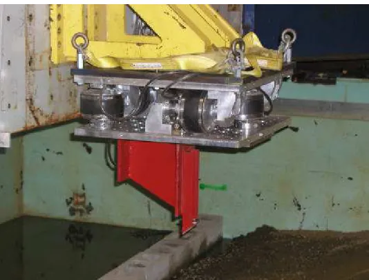
The loads on the ice block were measured using a 6-component dynamometer. Although only loads in one direction are required for this study, a dynamometer was used since it was already in place from the Phase 1 test series. The dynamometer is composed of six Interface load cells mounted in different configurations (Figure 9). This dynamometer consists of three load cells mounted to measure forces in the z-direction, two in the x-direction and one in the y-direction. For the present study, only the load output from the x-direction load cells were used. A steel bracket was mounted onto the bottom of the dynamometer to support one end of a chain that was connected to the ice block (see Figure 8).

The motions of the ice block were measured using the CHC-designed and manufactured MOTAN system (Figure 10 and Figure 11). The physical unit is made up of three accelerometers and three angular rate sensors housed in a unit that, in this case, was mounted onto a plywood base that sat on top of the ice model (Figure 11). The MOTAN system also includes a GEDAP computer

(16)

program that computes the angle and motion data from the input data (Miles, 2000).

The instrumentation was calibrated at the beginning of the test program to ensure reliable and accurate performance prior to installation in the model. Factory calibration constants were used for the dynamometers since in situ calibration was not possible. However, these factory constants were verified by a number of static tests. The data acquisition system (DAS) recorded the analog signals from all of the instrumentation. The signals were sampled and digitized by a NEFF Instruments System 100 data acquisition system. The data was sampled at a rate of 100 Hz. During sampling, an analog low-pass filter with a cut-off frequency of 33 Hz was applied to prevent aliasing. The digitized signals were recorded on a Digital VAX AlphaStation computer as GEDAP data files (Miles, 1990). GEDAP is a software package developed at the CHC to facilitate experiment control, data acquisition, data analysis and the graphical presentation of time series data.

Figure 9 Dynamometer mounted on main carriage, with the steel bracket that was used to support the chain

(17)

13 cm 1.25 cm 20.7 cm 39 cm 10.2 cm X ab Exposed Ice Plywood mold Centre of buoyancy

MOTAN reference point

MOTAN

Mounting unit for MOTAN

Direction of Motion

38 cm

Figure 10 Sketch of MOTAN set-up with respect to ice block.

(18)

The ice block was stored in a small cold room between tests and moved into the environmental chamber using a forklift for each test. Once in the chamber, the ice was lifted using a crane into the ice tank, where it was floated into position. The chain to attach the model to the main carriage was then clipped onto the model, and the model was loosely tethered to the main carriage and the service carriage as a safety precaution to prevent it from rolling so far as to submerge the MOTAN.

All of the instrumentation was re-zeroed before each test with everything held stationary. When this was completed, the data acquisition system (DAS) was started, and the ice block was pulled along the ice tank at the set speed. After the carriage had travelled the length of the channel for the test, it was stopped along with the DAS system. Figure 12 and Figure 13 show the overall set-up for the test series.

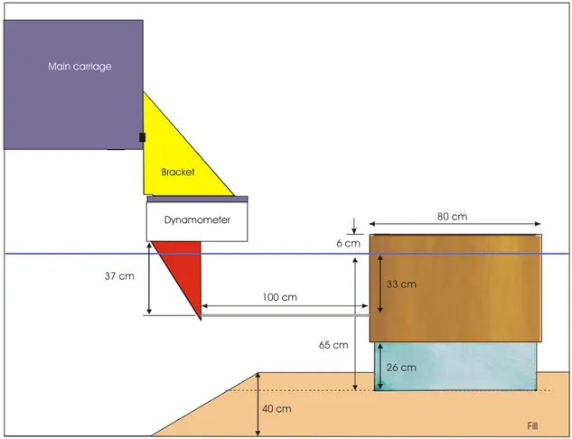
40 cm Fill Dynamometer 65 cm Bracket Main carriage 6 cm 100 cm 26 cm 33 cm 80 cm 37 cm

(19)

Figure 13 Test set-up showing the floating ice block with the MOTAN mounted on top. During a test, the ice block was towed approximately 1 m

behind the dynamomter. 2.6 Still Photographs and Video Clips

A video camera was housed in a waterproof casing and hand held throughout each test. This provided information on the scouring process occurring at the seabed. Also, a digital video camera was used to record the motions of the iceberg as seen above the water. The underwater video files were converted to .avi files. Between each series of tests, after the water was drained from the ice tank, photos were taken of each of the scour tracks. All of the video clips and still photographs (in .jpg format) are available on a CD-ROM.

(20)

2.7 Analysis of Measured Data 2.7.1 Scour Profiles

Certain measurements of the scour profile were taken after the tank was drained between tests. Profiles were taken in roughly the same location every time. The measurements were:

• Scour length taken along centerline of scour

• Scour depth (initial)

• Tongue length (length of ride-up out of trough, taken along centerline)

• Crest-to-crest width (average)

• Trough width (average)

• Outside-to-outside width (average)

• Inside crest height (average)

• Outside crest height (average)

Scour profile data were recorded on paper and then entered into an Excel worksheet. The data were then plotted as an average profile height versus distance across the scour track.

2.7.2 Force Data

Force data collected from the data acquisition system were transferred from the VAX unit to PC, where they were analyzed as follows:

• The measured data file was de-multiplexed to separate it into individual discrete data files. All data from a test are stored as voltages in a single multiplexed file. De-multiplexing creates a separate time-series data file for each channel and converts the voltages to physical units according to the predefined calibration equations and calibration constants for each channel.

• The data was time-selected to analyse two different situations that were observed in the tests, viz, (1) when the iceberg was scouring the seabed, and (2) when the iceberg was sliding along the seabed.

• The forces in the x-direction were summed from the two load cells measuring force in that direction.

• A statistical analysis was done on the time-selected portion of the force time-series and on the MOTAN data (see below) to provide information on the average, minimum and maximum values. In addition, for the situation were the iceberg was sliding on the seabed, the force data were fit to a probability distribution curve allowing probability values to be determined. Information is supplied on the 98% and 99% values. These values represent estimates of the “peak” value, and in general, are more reliable than the maximum measured value (since they use the whole time series). The probability density histogram and the cumulative distribution were computed from the data. The histogram was fit to 21 bins. The cell width was set according to the theoretical probability density function with a Gaussian distribution. The following symbols are used to define the quantities:

(21)

µ – the average value of the time-series. σ – the standard deviation of the time series. Min – the minimum measured value.

98%– the value of the parameter at the 98 percentile fit to a distribution curve

99%– the value of the parameter at the 99 percentile fit to a distribution curve

max– the maximum measured value.

It should be noted that when the iceberg was scouring this approach is not completely applicable, since this analysis assumes a Gaussian distribution of the loads. This was not the situation for the scouring process. However in the analysis, the maximum scour loads were compared with the 98% load for interest’s sake.

• The force results were plotted in a standard format. 2.7.3 MOTAN Data

The data collected using the MOTAN were analysed using the MOTAN’s accompanying GEDAP analysis package. The program computes the surge, sway, heave, roll, pitch and yaw motions obtained from the data (Miles, 2000). The input data required for the program, aside from the collected data, included the yaw angle at with the MOTAN unit was attached to the ice block, and the x, y and z co-ordinates of the vector that defines the position of the location where the motions were to be computed with respect to a reference point on the MOTAN base-plate. For these tests, the location about which the motions were to be computed was the centre of buoyancy of the model.

The output data for the test program consists of two plots per test, one detailing the time-series trace of the angles (roll, pitch and yaw) and the other of the motions (surge, sway and heave) of the ice block. As previously mentioned, statistical analysis of the time-series data traces was also performed. When the data acquisition system was re-zeroed at the beginning of every test, the ice block floating roughly in the same location, free to move with any small disturbances from the water in the ice tank. In order to accommodate these small movements, the time interval for re-zeroing the data was set to one or two minutes. Due to discrepancies between the position the ice block was floating in while the data acquisition system was being re-zeroed and the position the block was in as the test was underway, not all of the motion data were centred about zero on the y-axis. The data was therefore reset to have a zero-offset for ease of comparison between tests.

After the first test, it was noted that the ice block, after coming free of the seabed material, oscillated in a pitch mode for a number of seconds. A damped sine curve was fit to this section of the time record. The best-fit curve gave a damping ratio of 1% and a natural frequency of 0.34Hz (Figure 14).

(22)

Figure 14 Plot showing the free-vibration decay of the model. The “best fit” to the data indicated a natural frequency of 0.34 Hz and a damping

(23)

3. RESULTS

3.1 General Observation

All of the tests behaved in the same manner. Initially, the ice block was free-floating. When the ice block initially interacted with the edge of the seabed in the tank, it began to scour the seabed in a “bulldozing” manner. As the ice block continued to move, the scouring process continued but the ice block began to slowly heave and pitch. In this case the ice block pitched such that the front edge of the ice block was lower than the back edge. This behaviour continued for a while with the time depending upon the depth of the scour. At some point, as the seabed pileup became larger, the ice block began to pitch in the opposite direction. This caused the front of the iceberg to lift and ride-up onto the seabed. After this, the iceberg began to slide along the seabed. This remained the stable mode of the interaction process for the duration of the test. In this case, once the ice block was sliding along the seabed, there was no indication that it would begin to scour again.

The scour characteristics of this behaviour can be seen in Figure 15. It was evident that the preferred mode of motion of the iceberg was by sliding on the seabed and not be scouring. In some tests with the initial deep scours, the ice block was sliding along the seabed with approximately 17% of its total depth as freeboard (see Figure 16). The individual descriptions of each test are given in the following section.

Figure 15 Photo of Scour2_002 profile. The ice block travelled from the top left of the photograph to the bottom right.

(24)

a) b)

Figure 16 Photograph a) shows the amount of freeboard immediately before the ice block begins to scour during test Scour2_002, roughly 6 cm

to the top of the ice. Photograph b) shows the freeboard associated with the ice block as it slides along the surface of the seabed, now twice the

initial freeboard. 3.2 Description of the Tests

Seven tests were performed in this test series. The complete test matrix is shown in Table 1. The width of the exposed ice block changed due to a combination of melting and erosion.

Table 1 Test matrix File Name Ice Block Width

(m) Velocity (m/s) Cutting Depth (m) Angle of ice Block (°) scour2_002 0.76 0.05 0.05 0 scour2_003 0.76 0.05 0.1 0 scour2_004 0.72 0.15 0.1 0 scour2_005 0.72 0.05 0.2 0 scour2_006 0.68 0.05 0.15 45 scour2_007 0.68 0.05 0.15 0 3.3 Test Scour2_002

The water was set in the test basin to give a nominal scouring depth of 0.05 m. The velocity of the ice block was 0.05 m/s. A photo of the scour profile is shown in Figure 15. The 98% forces were 0.52 kN and 0.14 kN in the scouring and sliding sections respectively (Figure 17). Figure 18 and Figure 19 show the angle and motion data obtained from the MOTAN. Similar plots for the remaining tests may be found in the Appendix. All of the data were plotted using the same scale, for ease of comparison between tests.

(25)

Figure 17 Sum of forces in the x-direction for test Scour2_002

(26)

Figure 18 MOTAN angle results for test Scour2_002 Initial contact with seabed Beginning of sliding section

(27)

Figure 19 MOTAN motion results for test Scour2_002 3.4 Test Scour2_003

For the next test, the velocity of the ice model was again 0.05 m/s but the water depth was lowered to achieve a cutting depth of 0.1 m. The 98% force was 1.55 kN for the scour section, and 0.37 kN for the sliding section. Figure 20 shows the scour profile for this test.

Initial contact with seabed

Beginning of sliding section

(28)

Figure 20 Photo of Scour2_003 profile 3.5 Test Scour2_004

In this test, the ice block was again set to a 0.1 m scouring depth, but at a higher velocity – 0.15 m/s. The 98% force was 0.51 kN for scouring, and 0.33 kN for sliding.

3.6 Test Scour2_005

For this test, the model was run at 0.05 m/s at the deepest scouring depth of 0.2 m. The maximum 98% forces were 2.08 kN and 0.52 kN for the scour and sliding sections respectively.

3.7 Test Scour2_006

In order to assess if a different cutting face would affect how the model behaved, the model was turned 45° about the z-axis for the sixth test. In this case, the ice block was pulled with 2 ropes from the front edge. Unfortunately, when the model came into contact with the seabed material, scouring at a depth of 0.15 m, it dug in to such an extent that the MOTAN was in danger of becoming submerged in the water. The test in this configuration had to be abandoned. The rope configuration could have contributed to this behaviour. The forces that were observed during the brief test period indicated 98% forces of 1.76 kN and 1.34 kN for scour and sliding respectively.

3.8 Test Scour2_007

For the final test, the model was run at 0.05 m/s, with a cutting depth of 0.15m, through the same channel as the sixth test. The 98% forces were 0.62 kN for the scour section and 0.88 kN for the sliding section. A photo of the scour profile is shown in Figure 21.

(29)

Figure 21 Side view of Scour2_007 profile. The direction of motion of the iceberg was from left to right in the photograph.

(30)

4. ANALYSIS

4.1 Observational Data

As previously discussed, it was observed that after the model initially dug into the seabed, it gradually rode up the material and ended up skimming the top of the seabed for the majority of the test. This “chattering” was evident when the tank was drained after each test. An example of this is shown in Figure 22 and Figure 23 shows how the models rode up out of the seabed material.

Figure 22 Photo showing the chattering effect after the ice model rode up on top of the seabed material.

(31)

Figure 23 Scour2_002 and Scour2_003 4.2 Scour Profiles

Profile measurements were taken after most of the tests. These results are shown in Table 2. From the measurements, a rough sketch of the average scour profile for each test could be created. These profiles are shown in Figure 24. The crest heights for the tests run at 0.05 m/s were similar, while the crest height for the test run at 0.15 m/s was much smaller than the other tests. The distance traveled before the model rode up onto the seabed also varied between tests, however, there did not appear to be a consistent trend to the length of the scour path.

(32)

Table 2 Profile Measurements

Test Scour2_002 Scour2_003 Scour2_004 Scour length (cm) 183 341 82

Tongue length (cm) 75 106

Crest to crest (cm) 83 90 80

Trough width (cm) 63 50 76

Outside crest height (cm) 4 7.25 1.7

Inside crest height (cm) 5.6 9.25 2.5

Outside to outside (cm) 94 110.5 88

Slope 0.11 0.18 0.02

Trapezoidal Area (m²) 0.6862 0.7735 0.6864

Test Scour2_005 Scour2_006 Scour2_007 Scour length (cm) 285 n/a 215

Tongue length (cm) 77 n/a 93

Crest to crest (cm) 86 n/a 84

Trough width (cm) 52 n/a 55

Outside crest height (cm) 5 n/a 5

Inside crest height (cm) 8.8 n/a 6

Outside to outside (cm) 101 n/a 102

Slope 0.17 n/a 0.14

Trapezoidal Area (m²) 0.6969 n/a 0.7089

0 5 10 15 20 25 30 35 40 45 50 0 20 40 60 80 100 120 140

Width Across Scour (cm)

Depth of Scour (cm)

Scour2_002 Scour2_003 Scour2_004 Scour2_005 Scour2_007

(33)

4.3 Force Data

The force data showed that the highest forces for each test occurred after the model’s initial contact with the seabed material. Had the model not rode up onto the seabed each time, it is likely that the measured forces would have been much higher. Table 3 shows a summary of the measured force statistics. As it was, the maximum measured force was 2.25 kN, which occurred when the model was scouring at a depth of 0.2 m. The peak measured forces were much lower than the forces observed in the first phase of the study, by as much as a factor of six (Barker and Timco, 2002). Maximum and 98% forces are shown in Figure 25 and Figure 26.

Table 3 Summary of measured loads

Test Max.Force (kN) 98% Force (kN) Scour depth (m) Velocity (m/s) Scour2_002 scour 0.59 0.52 0.05 0.05 slide 0.26 0.14 0.05 Scour2_003 scour 1.68 1.55 0.1 0.05 slide 0.48 0.37 0.05 Scour2_004 scour 1.16 0.51 0.1 0.15 slide 0.42 0.33 0.15 Scour2_005 scour 2.25 2.08 0.2 0.05 slide 0.72 0.52 0.05 Scour2_006 scour 1.93 1.76 0.15 0.05 slide 1.4 1.34 0.05 Scour2_007 scour 0.89 0.62 0.15 0.05 slide 1.11 0.88 0.05

(34)

0.0 0.5 1.0 1.5 2.0 2.5 0.00 0.05 0.10 0.15 0.20 0.25 Scour Depth (m) Force (kN) 98% Force (kN) Max.Force (kN) Scouring

Figure 25 Maximum and 98% peak forces for scour section

0.0 0.5 1.0 1.5 2.0 2.5 0.00 0.05 0.10 0.15 0.20 0.25 Scour Depth (m) Force (kN) 98% Force (kN) Max.Force (kN) Sliding

(35)

4.4 MOTAN Data

For most of the tests, the MOTAN data analysis indicated that heave displacements were the largest of the three displacement measurements that were taken as the ice was pulled through the seabed material. This is consistent with the visual observations, especially as the model rode up out of the scour trough. Once on top of the seabed, the model bobbed up and down slightly as it was being towed. Surge movements were also observed as the chain connecting the ice model to the bracket below the dynamometer slackened and became taught over the length of the test.

With respect to angles, pitch and yaw motions dominated in all of the tests. As expected, pitch was especially prevalent at the initial contact of the ice with the seabed. For the tests at a higher velocity or at a deeper scouring depth, the model pitched a great deal at the contact point; from 5° to 10° past the model’s neutral position.

(36)

5. FINAL COMMENTS

A laboratory program has been performed to examine the ice scouring process of a floating ice model, through representative Grand Banks materials. This data is a supplement to a previous study that examined similar processes, but used ice models that were rigidly pushed through the material.

These free-floating tests provided some surprising results. In all cases it was evident that the ice block would move in such a manner so as to reduce the overall scouring forces on it. In this case, this led to the ice block sliding along the seabed. If this process occurs often in nature, it has serious implications with respect to sub-sea facilities and pipelines. First of all, although there was evidence of the sliding process on the seabed, the depth of the resulting “scour” was very small and would probably be difficult to detect using present-day profiling equipment. This non-detection could affect a probabilistic analysis of relic scours since these sliding scours would not be included. Secondly, the sliding iceberg loses some of its buoyancy and this loss of buoyancy is directly transferred to the seabed. This would result in significant additional vertical loading on the seabed.

The data sets from the CHC test program will be analyzed in more detail in the future. The analysis will be done in conjunction with the Geological Survey of Canada – Atlantic to investigate and review the full-scale scour signatures. This research may shed more insight into the scouring processes and the implications for sub-sea facilities on the Grand Banks of Canada.

(37)

6. ACKNOWLEDGEMENTS

The support of the Program on Energy Research and Development (PERD) through the Ice-Structure Interaction Program Activity is gratefully acknowledged. The research was carried out with the collaboration of Gary Sonnichsen and Ned King of the Geological Survey of Canada and discussions with them were extremely instructive. The assistance of two work term students from Memorial University of Newfoundland is acknowledged and appreciated. Stuart Gill designed and constructed the profiler and wooden moulds. Denise Sudom helped in collecting and analyzing the data. The 6-component dynamometer was designed by Ed Funke of COMDOR Engineering and fabricated in house at NRC.

(38)

7. REFERENCES

Barker, A. and Timco, G. (2002) Laboratory Experiments of Ice Scour Processes. PERD Report 32-28/CHC Report CHC-TR-004. Ottawa, Canada.

Davies, M.H. (2002) Iceberg Scour Study Final Report. Ottawa, Canada.

Miles, M.D. (1990) The GEDAP Data Analysis Software Package. NRC Report TR-HY-030, Ottawa, Canada.

Miles, M.D. (2000) Ship Motion Analysis Software for use with the MOTAN Inertial Motion Sensor Unit in the Icebreaking Research Ship USCGC Healy. NRC Confidential Report TR-HY-030. Ottawa, Canada.

Pratte, B. and Timco, G. (1981) A New Model Basin for the Testing of Ice-Structure Interactions. Proceedings POAC’81, Vol.2, pp 857-866, Quebec City, Canada.

Sonnichsen, G. and King, E. (2001) Surficial Sediments, Grand Bank, Offshore Newfoundland. PERD/CHC Report 31-27. Geological Survey of Canada, Dartmouth, Canada.

(39)

(40)

(41)

(42)

(43)

(44)

(45)

(46)

(47)

(48)

(49)

(50)

(51)

(52)

(53)

(54)

(55)

(56)

(57)

(58)

(59)

(60)

REPORT No./N°. DU RAPPORT CHC-TR-006 PROJECT No./No. DU PROJET 59581 SECURITY CLASSIFICATION/ CLASSIFICATION DE SÉCURITÉ

___ Top Secret/Très sécret ___ Secret ___ Confidential/Confidentiel ___ Protected/Protégée _x_ Unclassified/Non classifiée DISTRIBUTION/DIFFUSION ___ Controlled/Contrôlée _x_ Unlimited/Illimitée

DECLASSIFICATION: DATE OR REASON/DÉCLASSEMENT: DATE OU RAISON

TITLE, SUBTITLE/TITRE, SOUS-TITRE

Laboratory Experiments of Ice Scour Processes: Buoyant Ice Model AUTHOR(S)/AUTEUR(S)

Anne Barker and Garry Timco SERIES/SÉRIE

CORPORATE AUTHOR/PERFORMING ORGANIZATION/ AUTEUR D'ENTREPRISE/AGENCE D'EXÉCUTION

SPONSORING OR PARTICIPATING AGENCY/AGENCE DE SUBVENTION OU PARTICIPATION

Program on Energy Research and Development (PERD) DATE

May 2002

FILE/DOSSIER SPECIAL CODE/CODE

SPÉCIALE PAGES 59 FIGURES 26+ REFERENCES 6 NOTES

DESCRIPTORS (KEY WORDS)/MOTS-CLÉS

Ice scour processes, modelling, iceberg, Grand Banks, buoyant model SUMMARY/SOMMAIRE