Publisher’s version / Version de l'éditeur:
Vous avez des questions? Nous pouvons vous aider. Pour communiquer directement avec un auteur, consultez la première page de la revue dans laquelle son article a été publié afin de trouver ses coordonnées. Si vous n’arrivez pas à les repérer, communiquez avec nous à [email protected].
Questions? Contact the NRC Publications Archive team at
[email protected]. If you wish to email the authors directly, please see the first page of the publication for their contact information.
https://publications-cnrc.canada.ca/fra/droits
L’accès à ce site Web et l’utilisation de son contenu sont assujettis aux conditions présentées dans le site LISEZ CES CONDITIONS ATTENTIVEMENT AVANT D’UTILISER CE SITE WEB.
Proceedings of the Sixth Workshop on NLP for Similar Languages, Varieties and
Dialects, pp. 17-25, 2019
READ THESE TERMS AND CONDITIONS CAREFULLY BEFORE USING THIS WEBSITE. https://nrc-publications.canada.ca/eng/copyright
NRC Publications Archive Record / Notice des Archives des publications du CNRC : https://nrc-publications.canada.ca/eng/view/object/?id=e6334b65-1734-4c0e-86da-7fb23d5cf6be https://publications-cnrc.canada.ca/fra/voir/objet/?id=e6334b65-1734-4c0e-86da-7fb23d5cf6be
NRC Publications Archive
Archives des publications du CNRC
This publication could be one of several versions: author’s original, accepted manuscript or the publisher’s version. / La version de cette publication peut être l’une des suivantes : la version prépublication de l’auteur, la version acceptée du manuscrit ou la version de l’éditeur.
For the publisher’s version, please access the DOI link below./ Pour consulter la version de l’éditeur, utilisez le lien DOI ci-dessous.
https://doi.org/10.18653/v1/W19-1402
Access and use of this website and the material on it are subject to the Terms and Conditions set forth at
Improving cuneiform language identification with BERT
Bernier-Colborne, Gabriel; Goutte, Cyril; Léger, Serge
17
Improving Cuneiform Language Identification with BERT
Gabriel Bernier-Colborne, Cyril Goutte, Serge L´eger National Research Council Canada
{Gabriel.Bernier-Colborne, Cyril.Goutte, Serge.Leger}@nrc-cnrc.gc.ca
Abstract
We describe the systems developed by the National Research Council Canada for the Cuneiform Language Identification (CLI) shared task at the 2019 VarDial evaluation campaign. We compare a state-of-the-art base-line relying on character n-grams and a tradi-tional statistical classifier, a voting ensemble of classifiers, and a deep learning approach us-ing a Transformer network. We describe how these systems were trained, and analyze the impact of some preprocessing and model es-timation decisions. The deep neural network achieved 77% accuracy on the test data, which turned out to be the best performance at the CLI evaluation, establishing a new state-of-the-art for cuneiform language identification.
1 Introduction
The goal of the Cuneiform Language Identifica-tion (CLI) shared task (Zampieri et al.,2019) was to predict the language or language variety of a short segment of text written using cuneiform symbols. These language varieties include Sume-rian (SUX) and 6 different dialects of Akkadian: Old Babylonian (OLB), Middle Babylonian pe-ripheral (MPB), Standard Babylonian (STB), Neo Babylonian (NEB), Late Babylonian (LTB), and Neo Assyrian (NEA). The dataset for the shared task was built from the Open Richly Annotated Cuneiform Corpus,1 as described by Jauhiainen et al.(2019).
The NRC-CNRC team submitted 3 systems to the CLI shared task. The first one is a standard approach using Support Vector Machines (SVM) trained on character n-grams. The second one is an ensemble using plurality voting among several classifiers trained on different feature sets. This is essentially the approach that reached state-of-the-art on previous discriminating similar languages
1[http://oracc.museum.upenn.edu]
(DSL) shared tasks (Goutte et al., 2014, 2016). Our last submission is a deep learning approach based on character embeddings and a Transformer network, similar to BERT (Devlin et al.,2018).
The following section quickly reviews related work. We then describe the dataset and data pro-cessing (Section 3) and the systems we built for the shared task (Section4), before presenting the experimental results in Section5.
2 Related Work
Jauhiainen et al. (2018c) provide a thorough sur-vey of research on language identification. Re-garding the state-of-the-art, they point out that ”generally speaking, linear-kernel SVMs have been widely used for [language identification], with great success across a range of shared tasks” (Jauhiainen et al., 2018c). These SVMs usually exploit character n-grams as features.
Given that text segments in the CLI dataset (see Section3) are often very short, it is worth noting that the character-level language model-based sys-tem ofJauhiainen et al.(2016) achieved state-of-the-art results on texts longer than 25 characters, according to an empirical comparison of 7 meth-ods on 285 different language varieties ( Jauhi-ainen et al., 2017). On shorter texts containing less than 20 characters, the method of Vatanen et al.(2010), using a naive Bayes classifier based on smoothed character n-gram probabilities, per-formed better.
Jauhiainen et al. (2018c) point out that the use of neural networks for language identifica-tion has increased since 2016, with varying suc-cess. Medvedeva et al.(2017) compared SVMs to a feed-forward neural network that takes as input the average embedding of the character n-grams in the text, trained using multi-task learning, and found that ”traditional models, such as SVMs,
per-18 form better on this task than deep learning tech-niques” (Medvedeva et al.,2017, p. 161). On the other hand,Ali(2018) used character-level CNNs and RNNs and obtained strong results at VarDial 2018 (Zampieri et al., 2018), including second place on 2 dialect identification tasks (for Arabic and German). To our knowledge, we are the first to apply the recently proposed BERT method (Devlin et al., 2018) to the language identification prob-lem.
3 Data
As this was a closed task, the only data we used is the Cuneiform Language Identification dataset created for this task (Jauhiainen et al.,2019). The training set provided is unbalanced, the number of cases per class ranging from 3803 (OLB) to 53,673 (SUX). On the contrary, the development set is balanced, containing 668 cases for each class. See Table1for full statistics.
One challenging aspect of the data is that most of the text segments are very short. The segments in the training set contain only 7 characters on av-erage. More than half of the segments contain 5 characters or less, and more than 10% contain a single character. On the tail end of the distribution, a dozen segments contain more than 64 characters, and only one contains more than 128 characters. Again, the dev set is significantly different, as all segments with less than 3 characters were filtered out.
Another challenging aspect of this data is the low frequency of many of the cuneiform symbols. The training data contains 550 unique characters. 39 of these only appear once, and 128 appear 10 times or less. If we look at the development set, we find that it contains 365 unique characters, and 3 of these are not found in the training data.
One other important property of the training data is that it contains many duplicates, both within classes and between classes. The training set contains 139,421 segments, but only 86,454 are unique. The most frequent segment appears 3223 times, in 6 of the 7 classes. The second most fre-quent appears 1460 times, always in the same class (LTB).2
We processed the training and development sets provided to create our own cross-validation folds. Before creating the folds, we applied a
dedupli-2Note that this means that almost 10% of the examples in
the LTB class are the same text.
# segments Class raw dedup SUX 54,341 22,240 OLB 4,471 3,901 MPB 6,176 5,578 STB 18,485 16,327 NEB 10,375 8,595 LTB 16,615 8,665 NEA 33,634 26,614 Total 144,097 91,920
Table 1: Number of segments per class (train+dev), be-fore (raw) and after (dedup) deduplication.
cation step to the combined training and develop-ment data using the following strategy: we kept only one instance of every (segment, label) pair; for segments belonging to all 7 classes, however, we only kept one labeled instance, where the label is the most frequent label for that segment. The resulting per-class statistics are provided in Table
1.
We then folded the deduplicated data (contain-ing both the train(contain-ing and dev sets). Since the of-ficial development set was balanced, and we sus-pected the test set would be likewise, we created our folds such that the test set (and dev set) of each fold were balanced, containing mk (rounded to the nearest whole number) examples in each class, where m is the minimum class frequency in the combined training and development data, and k is the number of folds. With k = 5 and m = 3901, we obtained dev and test sets contain-ing either 780 or 781 examples for each class. This is larger than the official development set, and thus the training sets are smaller than the official train-ing set.
Note that during development of our deep learn-ing approach, we decided to fully deduplicate the training data, keeping only the most frequent label for each segment.
The cross-validation folds were used as follows to train the models: parameters were estimated on the training part of each fold, the dev part was used for setting extra parameters, e.g. for classi-fier calibration (see Section 4), and the test part was used to provide an unbiased estimate of the resulting performance. Note that, as specifically encouraged by the shared task organizers, the final systems were retrained on the combined training and development sets.
4 Methods
In this section, we describe the systems that we developed for the CLI task.
4.1 SVM-based models
Our SVM-based models exploit a straightforward pipeline that provides a strong baseline for lan-guage identification. This pipeline has three stages:
1. n-gram extraction and counting 2. feature weighting
3. estimation of calibrated statistical classifiers Extracting and counting character n-grams from cuneiform text is straightforward as there is no whitespace or punctuation requiring special pre-processing, e.g., tokenization. This is done for un-igrams, bun-igrams, trun-igrams, 4-grams and 5-grams. Note that for segments smaller than the n-gram size, the full segment is retained regardless of its size: the trigram corresponding to a segment of length 3 will therefore appear in the 4-gram and 5-gram feature spaces. We apply a feature weighting scheme combining log term frequency, inverse document frequency and cosine normal-ization, a.k.a. ltc in the SMART weighting scheme.3
One binary SVM classifier is trained for each of the seven classes in one-vs-all manner, weight-ing the minority class examples accordweight-ing to the ratio of class sizes. We then calibrate each classi-fier in order to produce proper probabilities. This is done using isotonic regression (Zadrozny and Elkan,2002), estimated on a left-out dev set. This allows the output of the 7 classifiers to be well-behaved probabilities that we can compare in or-der to predict the most probable class, or use in further post-processing in combination with other classifier’s outputs. The best model, as estimated by cross-validation, used n-grams of length 1 to 4, which we denote later by char[1-4].
Note that we also tried a two-stage approach similar to that ofGoutte et al. (2014) using vari-ous class groupings (eg. Sumerian vs. Akkadian dialects), but this did not prove particularly help-ful.
3[https://en.wikipedia.org/wiki/SMART_ Information_Retrieval_System]
4.1.1 Voting ensemble
Ensemble methods have proven quite successful on language identification (Malmasi and Dras,
2018) and other language classification tasks (Goutte and L´eger, 2017). We therefore submit-ted a system that performs plurality voting among several classifiers. The base classifiers are ob-tained by training calibrated SVM classifiers, as described above, on various feature spaces com-bining n-grams of various lengths. We also trained probabilistic classifiers (similar to Naive Bayes) on the same feature spaces. Although the over-all performance of the probabilistic classifiers was consistently lower than that of the SVMs, they provide a valuable addition to the ensemble be-cause their prediction patterns are different from those of the SVMs.
The ensemble was built by adding base classi-fiers to the ensemble, in decreasing order of over-all performance, as long as the estimated voting performance, using a cross-validation estimator, increases. For our submission, the resulting vot-ing ensemble contains 15 base classifiers, among which 10 are SVM-based and 5 are probabilistic classifiers. That submission is referred to below as ‘voting ensemble’ or simply ‘Ensemble’ in ta-bles.
4.2 BERT approach
Our second approach is a slightly modified version of the BERT model (Devlin et al.,2018).
We train a deep neural network which takes se-quences of characters as input, using (partially) unsupervised pre-training, followed by supervised fine-tuning on the CLI training data. The network is composed of a stack of bidirectional Trans-former modules (Vaswani et al.,2017) which code the input sequence. The output of the en-coder is fed to an output layer, which varies from one stage of training to the next.
First, we pre-train the model on unlabeled text using 2 pre-training tasks: a masked language model (MLM) and sentence pair classification (SPC).
The MLM pre-training task is exactly as de-scribed by Devlin et al.(2018). The goal of this task is to predict symbols chosen at random based on all the other symbols in the segment. Note that for this language identification task, the MLM pre-training task might be viewed as learning a multi-language model, that is a single model that can
20 predict characters based on context for all 7 of the cuneiform language varieties, and must therefore learn the specific markers of each variety.
As for the SPC pre-training task proposed by
Devlin et al.(2018), we adapted it to account for the fact that the segments in the training data are not in sequential order and are not divided into documents. We therefore split the training data into 7 pseudo-documents corresponding to the 7 classes (different cuneiform language varieties), and the task is to predict whether 2 segments be-long to the same class. This is a very simple adap-tation, but it introduces a supervised signal into the pre-training task, as we use the CLI labels to split the data into pseudo-documents. Learning to pre-dict whether 2 segments belong to the same lan-guage should be helpful to predict the lanlan-guage variety used in a specific text, when we fine-tune the model on this task later on.
Thus, the first phase of pre-training uses an out-put layer (or head) for both the MLM and SPC tasks. The first is a softmax over characters, which takes as input the encoding of a segment, where the characters to predict have been masked. The second is a binary softmax, which takes as input the joint encoding of 2 sentences, which we join together using a special symbol that indicates the boundary between 2 sentences.
This is followed by a second phase of pre-training where we include the unlabeled test data in the training data. Since we don’t know the la-bels of the test data, it would not make sense to use the (modified) SPC task for pre-training, so we only use MLM, which is fully unsupervised with respect to the CLI task. We re-train the weights of the feature extractor (i.e. encoder) using a single head for MLM.
Once the model is fully pre-trained, we fine-tune it on the target task, i.e. to predict the lan-guage variety of each text, using the labeled train-ing and dev data. For this, we use the feature ex-tractor learned during the 2 phases of pre-training, and add a new head for language identification, which is simply a softmax over the 7 language va-rieties.
The vocabulary (or alphabet) is composed of ev-ery character in the Unicode range for cuneiform characters. Note that characters in the test data which were not in the training data can still be modeled to some extent because of the inclusion of the unlabeled test data during the second phase
of pre-training.
Our hyperparameter settings largely resemble those used byDevlin et al.(2018) (for their smaller model):
• Nb Transformer layers: 12 • Nb attention heads: 12 • Hidden layer size: 768 • Feed forward/filter size: 3072 • Hidden activation: gelu • Dropout probability: 0.1 • Max sequence length: 128 • Optimizer: Adam
• Learning rate for pre-training: 1e-4 • Batch size for pre-training: 64
• Training steps: 500K and 100K for pre-training (phases 1 and 2 respectively), and 20K for fine-tuning
• Warmup steps: 10K for both pre-training (phase 1 only) and fine-tuning
As for the fine-tuning stage, we do a small grid search, over the following hyperparameter set-tings:
• Batch size: {16, 32}
• Learning rate: {1e-5, 2e-5, 3e-5, 5e-5} We did a few ad hoc tests on our own devel-opment set (using one of the folds we created for cross-validation) to assess the impact of dedupli-cation and the various pre-training strategies (us-ing SPC or not, do(us-ing a second phase where we in-clude the test data), which is how we arrived at our final model. We also tuned the number of train-ing steps for fine-tuntrain-ing on this dev set. We will not present the results of these tests here, but will show the results of ablation tests we conducted on the official dev set in Section5.3.
Note that our final model was fine-tuned on the combined training and dev set, which we fully deduplicated, by keeping only one instance of each text, along with its most frequent label. The unlabeled test set examples were also used during the second phase of pre-training.
Our code is available at https://github. com/gbcolborne/lang_id.
5 Results
We discuss the results of our official submissions in the following section. We also analyze the impact of various high-level modelling decisions, look at potential sources of errors, and conduct some ablation tests.
5.1 Test results
The scores of our 3 official submissions on the test set are shown in Table 2. Our best scores were achieved by the deep learning approach. This run was ranked first overall. Our voting ensemble would have been ranked 2nd, and our single SVM would have been ranked 3rd.
System F1 (macro) Accuracy Jauhiainen (2019) 0.7206
-char[1-4] 0.7414 0.7453
Ensemble 0.7449 0.7494
BERT 0.7695 0.7711
Table 2: Results of our 3 official runs on the CLI test set. For comparison, best F-score from (Jauhiainen et al.,2019)
The BERT model achieves an absolute gain of almost 2.5 F-score points over the voting ensem-ble. As for the voting ensemble, it produced an absolute gain of 0.35 F-score points over the best single SVM.
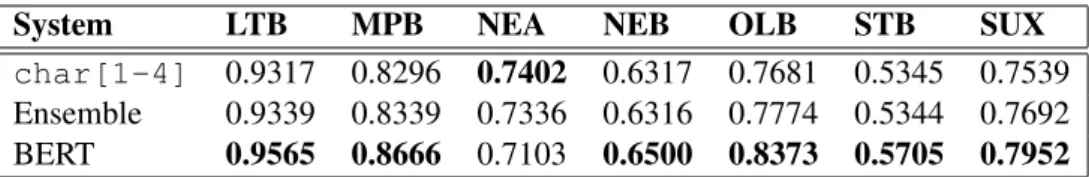
A detailed breakdown of our results on each of the 7 classes (languages) is presented in Ta-ble 3. These results show that the deep learning approach produces the best results on all but one of the classes, sometimes by quite a margin (e.g. OLB).
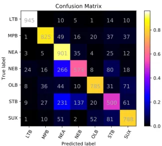
The 3 classes on which our scores are lowest are Standard Babylonian (STB), Neo Babylonian (NEB), and Neo Assyrian (NEA). As we can see in the confusion matrix for our best run, illustrated in Figure1, the BERT model often confuses both NEB and STB texts as NEA, which may be partly due to the fact that NEA is the most frequent class in the deduplicated training data.
5.2 SVM performance anaysis
We relied on a cross-validation estimate described in Section3in order to guide several high-level de-cisions, as described in Section4. Official shared task results (see Table2), however, turned out to be significantly lower than the cross-validation es-timate we based our decisions on. This raises the
LTB MPB NEA NEB OLB STB SUX Predicted label LTB MPB NEA NEB OLB STB SUX True label 945 10 5 1 14 10 1 825 49 16 20 37 37 3 5 901 35 4 25 12 24 16 266 573 8 80 18 8 36 44 10 785 31 71 9 27 231 137 20 500 61 1 10 51 2 52 81 788 Confusion Matrix 0.0 0.2 0.4 0.6 0.8
Figure 1: Confusion matrix for our best run (BERT) on the CLI test set.
question of how different the estimate would have been had we relied on the official dev set instead of full cross-validation, and whether this may have changed our decisions, for example with respect to which model to submit.
Another issue is the segment duplication men-tioned in Section3as well as byJauhiainen et al.
(2019). Removing duplicated segments makes the training data more similar to the dev and test sets, however, it also greatly reduces the amount of seg-ments available for training our models. We inves-tigate this trade-off by re-training a few key mod-els on the original training data, without perform-ing any deduplication. For these comparisons, we use our best single model, char[1-4], the next best single model, char[1-3], and the voting ensemble.
Table 4 shows the results of these experi-ments. It turns out that the performance estimated by cross-validation is consistently 12–13 points higher than the performance estimated on the dev set. Note also that contrary to Jauhiainen et al.
(2019), who report marginally better F-scores on the dev than on the test set, we obtained 3–4 points higher F-score on the final test set than on the dev set.
Comparing the results obtained on raw vs. deduplicated training data, we see that the cross-validation estimate is about 1 point higher when models are trained on the deduplicated data, but the difference on the dev is much smaller (0.06– 0.22 points). For the voting ensemble, it turns out that dev performance is actually slightly better
22
System LTB MPB NEA NEB OLB STB SUX
char[1-4] 0.9317 0.8296 0.7402 0.6317 0.7681 0.5345 0.7539 Ensemble 0.9339 0.8339 0.7336 0.6316 0.7774 0.5344 0.7692 BERT 0.9565 0.8666 0.7103 0.6500 0.8373 0.5705 0.7952
Table 3: Class-wise F-score of our 3 official runs on the CLI test set.
CV Dev
System raw dedup raw dedup
Ensemble 0.8345 0.8431 0.7114 0.7092 char[1-3] 0.8226 0.8337 0.7055 0.7061 char[1-4] 0.8241 0.8347 0.7006 0.7026
Table 4: Impact of estimating model performance (macro F1) on the cross-validation (CV) estimator vs. dev set, and impact of deduplicating the training data on the resulting performance. char[1-N] are single SVM models trained on n-grams of length 1 to N .
when duplicates are not removed from the training data.
Finally, one concern is whether these differ-ences would have an impact on model selection or high-level modelling choices. It turns out that ac-cording to dev set performance, the char[1-3] model is better than the char[1-4] model we submitted, by about half a point. It will be interest-ing to check whether this difference is matched on test performance, once reference labels are avail-able.
5.3 BERT ablation tests
We carried out a few simple ablation tests on the BERT model, using the official development set for validation and testing. We split this dev set into two random subsets of equal size, which we will call dev-A and dev-B. One half was used to optimize the number of training epochs (i.e. to do early stopping), and the other half was used as a held out test set, to get an unbiased estimate of the accuracy of the model.
These tests were meant to assess the impact of: • Using both MLM and SPC for pre-training
(phase 1)
• Doing a second phase of pre-training (MLM only) on both the training and dev data • Deduplicating the training data
We pre-trained 4 models on the official training set, one in the same manner as our official run, one
without SPC, one without deduplication, and one without SPC nor deduplication.
We then re-trained these 4 models on the com-bined training and dev sets (both halves). Only MLM was used (as we are using the dev set for evaluation, so we assume we don’t have the dev labels). Deduplication was applied only for the models that were initially pre-trained on dedupli-cated data.
We then fine-tuned the 8 resulting models (4 with re-training, 4 without) on the labeled training set. Again, we use deduplicated training data for the models that were pre-trained on deduplicated data.
For each of the 8 fine-tuning configurations, we did 5 replications of the fine-tuning phase using different seeds for the random number generators, to assess the impact of random initialization (note that the random initialization only affects the out-put head since the models were pre-trained). This is estimated by computing the 95% confidence in-terval on the scores obtained on the 5 runs.
We did these 5 replications twice, first with dev-A as dev set and dev-B as test set, then the other way around. This would allow us to evaluate the stability of the evaluation metrics over different sets of validation and test instances, as well as the stability of the optimal number of training epochs. This procedure is sometimes referred to as esti-mating “split-half reliability”. Note that our re-sults on either half of the dev set are not exactly comparable to results on the full dev set.
For these ablation tests, we reduced the batch size for pre-training from 64 to 48, due to time constraints and limited access to GPUs. For fine-tuning, we used a learning rate of 1e-5 and a batch size of 32.
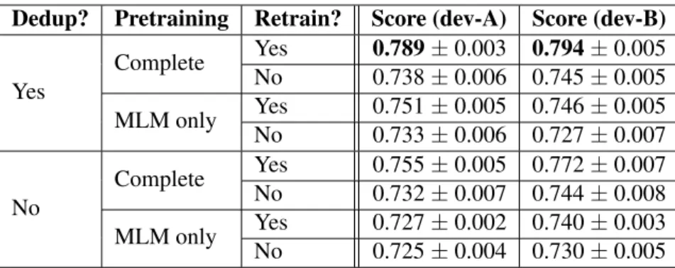
The results are shown in Table5. These results show that the biggest gains were obtained by doing a second phase of pre-training (with MLM only) on both the training and test data. If we only do the first pre-training phase, we lose about 5 points of F-score (absolute). If we drop SPC for pre-training (and use only MLM for both pre-pre-training
Dedup? Pretraining Retrain? Score (dev-A) Score (dev-B) Yes Complete Yes 0.789± 0.003 0.794± 0.005 No 0.738± 0.006 0.745± 0.005 MLM only Yes 0.751± 0.005 0.746± 0.005 No 0.733± 0.006 0.727± 0.007 No Complete Yes 0.755± 0.005 0.772± 0.007 No 0.732± 0.007 0.744± 0.008 MLM only Yes 0.727± 0.002 0.740± 0.003 No 0.725± 0.004 0.730± 0.005
Table 5: BERT ablation test results: mean F1 (macro) with 95% confidence interval. Retrain means the 2nd phase of pre-training (MLM only), which includes the unlabeled dev and test data.
phases), we lose 4-5 points as well. And if we don’t deduplicate the training data (and use both MLM and SPC for the initial pre-training), we lose 2-3 points.
It is important to note that if we optimized the other hyperparameters (notably the learning rate), the results we would achieve with these various training strategies would be different.
As for the number of training epochs, under the optimal training conditions (with dedup and full pre-training), the dev score peaked after only 1 or 2 epochs,4 and this result was stable across both test sets (i.e. dev-A and dev-B), the optimal num-ber of epochs being 1.2± 0.555 in one case and exactly 1.0± 0.0 in the other.
It would be interesting to see if the SVM-based model can reach the same accuracy as BERT if we adapt it to the test data, e.g. using self-training. The team ranked second on this CLI task used a form of self-training to adapt an SVM to the test data, and their F-score on the test set (0.7632) was not very far behind the score we achieved with BERT (0.7695). Furthermore, results of the German Dialect Identification and Indo-Aryan Language Identification tasks at Var-Dial 2018 (Zampieri et al., 2018) showed that the best results were obtained by systems that were adapted to the test data (Jauhiainen et al.,
2018a,b).
5.4 Error analysis
Using the predictions of the BERT model on dev-A,5 we analyzed the impact of text length on the error rate, as we suspected that the short length of the texts would be a major source of errors. This analysis showed that the error rate is around 32%
4
This suggests we should try an even smaller learning rate.
5Results on dev-B are similar.
for the shortest texts in dev-A (length 3), and falls to 12% for texts containing 10 characters. 83% of all errors were made on texts containing 9 charac-ters or less, 9.1 characcharac-ters being the average length of the texts in dev-A.
We also looked at the impact of OOV charac-ters, but this is not a significant source of errors, as only 3 texts in the official dev set contain a char-acter that was not seen during training.
Finally, we checked if any of the texts in the official dev set were seen during training, and this was the case for 574 of 4676 texts. Of these 574 cases, we find 49 cases where the label in the dev set was not seen during training, and 6 additional cases where the training labels of a text contained not only the dev label, but others as well. Thus, we could say that label ambiguity (in other words, multiple class membership) was a source of errors for a little over 1% of texts in the dev set.
6 Conclusion
In this paper, we described the systems built by the NRC-CNRC team for the Cuneiform Language Identification shared task at the 2019 VarDial eval-uation campaign. We adapted the BERT model to the language identification task, and compared this deep learning approach to statistical classifiers trained on character n-grams, which have long provided a strong baseline for language identifi-cation tasks. Our results using the BERT model surpass those obtained with an ensemble of clas-sifiers trained on different feature sets comprising n-grams of varying lengths, achieving an absolute gain of about 2.5 F-score points on the test set, and establishing the state-of-the-art for cuneiform language identification. This is largely due to the ability to conduct unsupervised learning on the test set before making predictions, as well as the
mod-24 ified sentence pair classification task we use for pre-training.
For future work, it would be interesting to model the shape of cuneiform symbols, or their transliterations, in order to better capture similar-ities between symbols. We also plan on testing BERT on other language identification datasets. Finally, we plan on casting this problem as a multi-label classification problem, as we believe this could be a better approach for the CLI task, and related tasks on discriminating similar languages.
References
Mohamed Ali. 2018. Character level convolutional neural network for arabic dialect identification. In Proceedings of the Fifth Workshop on NLP for Sim-ilar Languages, Varieties and Dialects (VarDial 2018), pages 122–127.
Jacob Devlin, Ming-Wei Chang, Kenton Lee, and Kristina Toutanova. 2018. BERT: pre-training of deep bidirectional transformers for language
under-standing. CoRR, abs/1810.04805.
Cyril Goutte and Serge L´eger. 2017. Exploring optimal
voting in native language identification. In
Proceed-ings of the 12th Workshop on Innovative Use of NLP for Building Educational Applications, pages 367– 373, Copenhagen, Denmark. Association for Com-putational Linguistics.
Cyril Goutte, Serge L´eger, and Marine Carpuat. 2014. The NRC system for discriminating similar lan-guages. In Proceedings of the First Workshop on Applying NLP Tools to Similar Languages, Varieties and Dialects (VarDial), pages 139–145, Dublin, Ire-land.
Cyril Goutte, Serge L´eger, Shervin Malmasi, and Mar-cos Zampieri. 2016. Discriminating Similar Lan-guages: Evaluations and Explorations. In Pro-ceedings of the Language Resources and Evaluation (LREC), Portoroz, Slovenia.
Tommi Jauhiainen, Heidi Jauhiainen, Tero Alstola, and Krister Lind´en. 2019. Language and Dialect Identi-fication of Cuneiform Texts. In Proceedings of the Sixth Workshop on NLP for Similar Languages, Va-rieties and Dialects (VarDial).
Tommi Jauhiainen, Heidi Jauhiainen, and Krister Lind´en. 2018a. HeLI-based experiments in Swiss German dialect identification. In Proceedings of the Fifth Workshop on NLP for Similar Languages, Va-rieties and Dialects (VarDial 2018), pages 254–262. Tommi Jauhiainen, Heidi Jauhiainen, and Krister Lind´en. 2018b. Iterative language model adapta-tion for indo-aryan language identificaadapta-tion. In Pro-ceedings of the Fifth Workshop on NLP for Similar Languages, Varieties and Dialects (VarDial 2018), pages 66–75.
Tommi Jauhiainen, Krister Lind´en, and Heidi Jauhi-ainen. 2016. HeLI, a Word-Based Backoff Method for Language Identification. In Proceedings of the Third Workshop on NLP for Similar Languages, Va-rieties and Dialects (VarDial3), pages 153–162, Os-aka, Japan.
Tommi Jauhiainen, Krister Lind´en, and Heidi Jauhi-ainen. 2017. Evaluation of language identification
methods using 285 languages. In Proceedings of the
21st Nordic Conference on Computational Linguis-tics, pages 183–191. Association for Computational Linguistics.
Tommi Jauhiainen, Marco Lui, Marcos Zampieri, Tim-othy Baldwin, and Krister Lind´en. 2018c. Auto-matic language identification in texts: A survey. arXiv preprint arXiv:1804.08186.
Shervin Malmasi and Mark Dras. 2018. Native lan-guage identification with classifier stacking and
en-sembles. Computational Linguistics, 44(3):403–
446.
Maria Medvedeva, Martin Kroon, and Barbara Plank. 2017. When sparse traditional models outperform dense neural networks: the curious case of discrimi-nating between similar languages. In Proceedings of the Fourth Workshop on NLP for Similar Languages, Varieties and Dialects (VarDial), pages 156–163. Ashish Vaswani, Noam Shazeer, Niki Parmar, Jakob
Uszkoreit, Llion Jones, Aidan N Gomez, Łukasz Kaiser, and Illia Polosukhin. 2017. Attention is all you need. In Advances in Neural Information Pro-cessing Systems, pages 5998–6008.
Tommi Vatanen, Jaakko J V¨ayrynen, and Sami Vir-pioja. 2010. Language identification of short text segments with n-gram models. In Proceedings of LREC.
B. Zadrozny and C. Elkan. 2002. Transforming clas-sifier scores into accurate multiclass probability es-timates. In Proceedings of the Eighth International Conference on Knowledge Discovery and Data Min-ing (KDD’02).
Marcos Zampieri, Shervin Malmasi, Preslav Nakov, Ahmed Ali, Suwon Shuon, James Glass, Yves Scherrer, Tanja Samardˇzi´c, Nikola Ljubeˇsi´c, J¨org Tiedemann, Chris van der Lee, Stefan Grondelaers, Nelleke Oostdijk, Antal van den Bosch, Ritesh Ku-mar, Bornini Lahiri, and Mayank Jain. 2018. Lan-guage Identification and Morphosyntactic Tagging: The Second VarDial Evaluation Campaign. In Pro-ceedings of the Fifth Workshop on NLP for Similar Languages, Varieties and Dialects (VarDial), Santa Fe, USA.
Marcos Zampieri, Shervin Malmasi, Yves Scherrer, Tanja Samardˇzi´c, Francis Tyers, Miikka Silfverberg, Natalia Klyueva, Tung-Le Pan, Chu-Ren Huang, Radu Tudor Ionescu, Andrei Butnaru, and Tommi Jauhiainen. 2019. A Report on the Third VarDial
Evaluation Campaign. In Proceedings of the Sixth Workshop on NLP for Similar Languages, Varieties and Dialects (VarDial). Association for Computa-tional Linguistics.