An Intermodel comparison of DDS and Daysim daylight coefficient models

Publisher’s version / Version de l'éditeur:

Vous avez des questions? Nous pouvons vous aider. Pour communiquer directement avec un auteur, consultez la première page de la revue dans laquelle son article a été publié afin de trouver ses coordonnées. Si vous n’arrivez pas à les repérer, communiquez avec nous à PublicationsArchive-ArchivesPublications@nrc-cnrc.gc.ca.

Questions? Contact the NRC Publications Archive team at

PublicationsArchive-ArchivesPublications@nrc-cnrc.gc.ca. If you wish to email the authors directly, please see the first page of the publication for their contact information.

https://publications-cnrc.canada.ca/fra/droits

L’accès à ce site Web et l’utilisation de son contenu sont assujettis aux conditions présentées dans le site LISEZ CES CONDITIONS ATTENTIVEMENT AVANT D’UTILISER CE SITE WEB.

EPIC 2006 AIVC, the 4th European Conference on Energy Performance & Indoor Climate in Buildings [Proceedings], pp. 1-6, 2006-11-01

READ THESE TERMS AND CONDITIONS CAREFULLY BEFORE USING THIS WEBSITE.

https://nrc-publications.canada.ca/eng/copyright

NRC Publications Archive Record / Notice des Archives des publications du CNRC :

https://nrc-publications.canada.ca/eng/view/object/?id=2137a94d-13fe-4bcd-be49-3ddbac0de37c https://publications-cnrc.canada.ca/fra/voir/objet/?id=2137a94d-13fe-4bcd-be49-3ddbac0de37c

NRC Publications Archive

Archives des publications du CNRC

This publication could be one of several versions: author’s original, accepted manuscript or the publisher’s version. / La version de cette publication peut être l’une des suivantes : la version prépublication de l’auteur, la version acceptée du manuscrit ou la version de l’éditeur.

Access and use of this website and the material on it are subject to the Terms and Conditions set forth at An Intermodel comparison of DDS and Daysim daylight coefficient models

http://irc.nrc-cnrc.gc.ca

An I nt e r m ode l c om pa rison of DDS a nd

Da ysim da ylight c oe ffic ie nt m ode ls

N R C C - 4 9 2 2 5

B o u r g e o i s , D . ; R e i n h a r t , C . F .

A v e r s i o n o f t h i s d o c u m e n t i s p u b l i s h e d i n

/ U n e v e r s i o n d e c e d o c u m e n t s e t r o u v e

d a n s : E P I C 2 0 0 6 A I V C , t h e 4

E u r o p e a n

C o n f e r e n c e o n E n e r g y P e r f o r m a n c e &

I n d o o r C l i m a t e i n B u i l d i n g s , L y o n , F r a n c e ,

N o v . 2 0 - 2 2 , 2 0 0 6 , p p . 1 - 6

An Intermodel Comparison of DDS and Daysim Daylight

Coefficient Models

D. Bourgeois

, C.F. Reinhart

National Research Council Canada

1200 Montreal Road, Ottawa (Ontario), K1A 0R6, CANADA denis.bourgeois@nrc-cnrc.gc.ca christoph.reinhart@nrc-cnrc.gc.ca

ABSTRACT

This paper presents the results of a Radiance-based intermodel comparison between the validated Daysim daylight coefficient model and a new standard model for dynamic daylighting simulations (DDS). The new model offers independence from site location and orientation, estimation techniques and simulation applications. The standard data can be used for dedicated daylighting analysis or for integrated building energy/daylighting simulation. Results show that DDS outperforms Daysim, notably in cases where sensors are subjected to sudden changes in solar exposure, e.g. for sensors far from a window.

INTRODUCTION

Daylight coefficients rely on dividing the celestial hemisphere into discrete sky segments and on calculating the contribution of each segment to the illuminance at a given sensor (Tregenza and Waters 1983). For sensor x, a daylight coefficient DCα (x) related to a sky segment Sα is defined as the illuminance, E, at x caused by the sky segment, Sα, divided

by its luminance, Lα, and its angular size, ΔSα. The total sensor illuminance, E(x), is obtained by linear superposition of each daylight coefficient coupled with the time-varying luminance of its matching segment (Equation 1). Time-time-varying solar and sky segment luminances can be calculated using meteorological data, luminous efficacy models (Perez et al. 1990), and luminous distribution models (Perez et al. 1993).

∑

Daylight coefficients can provide fast and accurate estimations of dynamic daylighting performance metrics (Reinhart et al. 2006), and energy savings from reduced electric lighting use, as well as heating and cooling (Janak and Macdonald 1999, Ajmat et al. 2005, Bourgeois et al. 2006). A number of packages today provide run-time coupling of daylighting simulation, yet these tools often manage daylighting and energy data under a single building model. Geometrical parameters for daylighting are often directly inherited from low-resolution descriptions of thermal zones, which can lead to incorrect solutions. Conversely, an architect or a lighting designer may come up with a novel solution with daylighting software, yet is unable to share the resulting high-quality

daylighting predictions with building energy simulationists. Regardless of the objective, a common mechanism for sharing dynamic daylighting simulation data would be beneficial. A new standard model of using daylight coefficients has been developed to address this impediment. The accuracy of the new model, DDS, is compared to Daysim1, another Radiance-based daylight coefficient model upon which DDS is based, as well Radiance2.

DEFINITION OF A STANDARD DAYLIGHT COEFFICIENT FORMAT

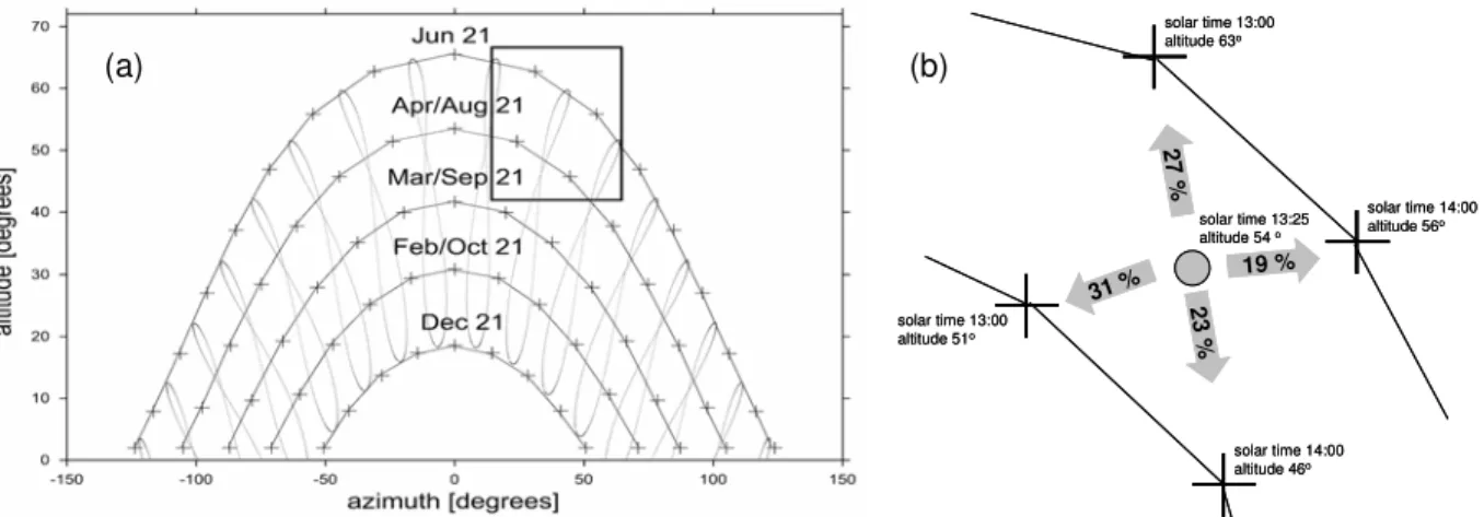
DDS daylight coefficients can be coupled with a sky model, e.g. the All Weather Perez model (1993), as described in Equation 2:

∑

∑

∑

The first part of Equation 2 is the diffuse contribution from the sky, necessitating a one-to-one mapping of 145 daylight coefficients to diffuse sky segments. DDS adopts the Daysim scheme of rectangular segments that completely cover the celestial hemisphere. The second daylight coefficient in Equation 2 represents the total diffuse ground contributions. Daylight coefficient models differ mainly in how solar contributions are considered. Daysim defines a set of around 65 latitude-dependent solar positions that form a grid among all solar positions throughout the year, as shown in Figure 1(a).

31 % solar time 13:00 altitude 63o solar time 14:00 altitude 56o solar time 13:00 altitude 51o solar time 14:00 altitude 46o solar time 13:25 altitude 54 o 2 7 % 19 % 2 3 % 31 % solar time 13:00 altitude 63o solar time 14:00 altitude 56o solar time 13:00 altitude 51o solar time 14:00 altitude 46o solar time 13:25 altitude 54 o 2 7 % 19 % 2 3 % (a) (b)

Figure 1: Daysim solar positions for Freiburg, Germany (47.979°N) (a): hourly mean solar positions with the crosses marking 65 solar positions. The box delineates the solar positions at 13:00 and 14:00 solar time on June and April/August 21st. (b): the interpolation algorithm to assign solar luminances to the four

positions on May 7th at 13:25. The crosses correspond to those within the box marked in (a).

At any given time, 4 of the 65 solar positions effectively circumscribe the sun. Daysim uses an interpolation algorithm whereby the calculated luminance from the sun is

1

irc.nrc-cnrc.gc.ca/ie/lighting/daylight/Daysim

2

distributed among these 4 solar positions, as a function of time and altitude differences (Figure 1 (b)). DDS considers indirect and direct solar contributions separately, as presented in Equation 23. DDS evenly distributes 145 indirect solar positions across the hemisphere, precisely at the centres of diffuse sky segments. As with Daysim, the 4 nearest indirect solar positions to the sun are chosen to determine the indirect solar contribution, with interpolation weights, wisun, based on their angular distances to the sun. Direct solar positions are also evenly distributed across the hemisphere, yet with greater resolution to increase simulation accuracy (Mardaljevic 2000). DDS comprises a default number of 2305 evenly-distributed direct solar positions, as indicated in Equation 24. Interpolation based on the solar angular distances of the 4 neighbouring direct solar positions is also used to calculate the direct solar contribution. The 2305 positions are obtained by quadrupling the original number of Tregenza horizontal rows of sky segments, then quadrupling the original number of Tregenza segments per row, while keeping a single zenith position5.

INTERMODEL COMPARISON

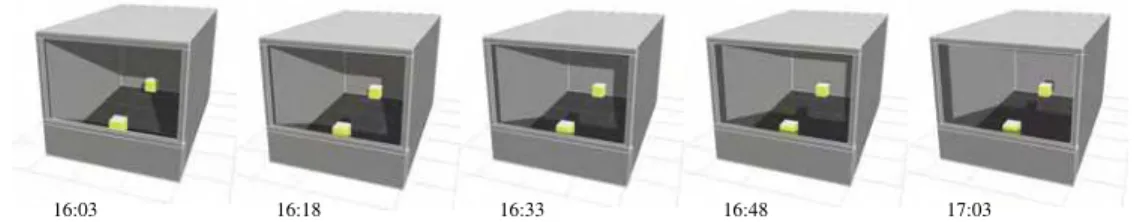
As both Radiance-based DDS and Daysim models differ only in direct solar position resolution, one would expect to find prediction discrepancies only in cases where sensors are subjected to sudden changes in solar exposure. Figure 2 illustrates the shifting solar patterns in an example office space between 16:03 and 17:03 on September 12th. The office has a depth of 4.7m, a width of 3.0m and a height of 2.8m. Floor, wall and ceiling reflectances are 20%, 50% and 80%, respectively. The west-facing façade is glazed above work plane height and has a glazing visual transmittance of 80%. The chosen site location is Vancouver, Canada (49.2°N, 123.2°W)6.

16:03 16:18 16:33 16:48 17:03

Figure 2: Shifting solar patterns in the west facing example office space between 16:03 and 17:03 on September 12, at 15 minute intervals. Two floating cubes, upon which two sensors (#1 and #10) are

centred, are illustrated for visual reference (images from Ecotect7)

The Daysim program gen_dc generated daylight coefficients for 14 upward-facing indoor sensors located along the room centreline, as well as an unobstructed upward-facing outdoor sensor, using both DDS and the original Daysim sky division schemes. Indoor

3

The indirect contribution comprises only solar rays that are reflected off surfaces, while the direct contribution consists only of the direct beam of sunlight that sees a sensor, excluding all reflected contributions.

4

A mechanism is provided to increase this number to take into account very detailed solar obstructions.

5 ( 144 x 4 x 4 ) + 1 = 2305 6 www.eere.energy.gov/buildings/energyplus/cfm/weather_data.cfm 7 www.squ1.com

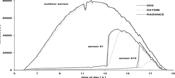
sensors are spaced apart by 0.3m, at a height of 0.85m. Illuminance time series using DDS and Daysim schemes, as well as conventional Radiance, during sunlit hours on September 12th are plotted in Figure 3 for sensors #1 (nearest to the window) and #10, as well as the unobstructed outdoor sensor8.

0 20000 40000 60000 80000 5 7 9 11 13 15 17 19 time of day [ h ] illu mi nanc e [ lux ] DDS DAYSIM RADIANCE outdoor sensor sensor #1 sensor #10

Figure 3: Predicted illuminances on September 12 for sensor #1 and #10 and an unobstructed outdoor sensor, for example office space (at 5 minute intervals)

Generally, results are identical for all sensors. Both DDS and Radiance predict a sudden spike in illuminance when the sun hits sensor #10 a few minutes after 16:00, peaking at around 30 000 lux. Daysim fails to predict this spike, going up to around 10 000 lux. This discrepancy is attributable to each model's prediction of cast shadows from architectural features, such as the window frame in the example application. If a sensor is sunlit yet one or more of the four neighbouring positions is not in direct line of sight with the sensor, than the interpolation algorithm will systematically introduce prediction errors, as positions that do see a sensor have direct solar contributions of 0. Solar positions at 16:00 and 17:00 on August and September 21st comprise the four nearest Daysim positions on September 12th during that hour, yet two of these do not actually see sensor #10 at 16:00 (on September and August) given the resolution of solar positions. As a result, Daysim yields lower results than DDS and Radiance during this time interval.

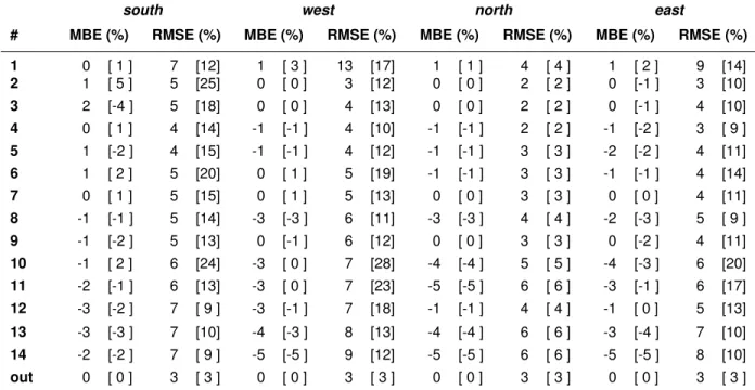
For more insight, DDS and Daysim daylight coefficients for all 15 sensors were calculated for south, east and north facing variants of the initial example office space9. Annual illuminance time series for all sensors were subsequently calculated using the resulting DDS and Daysim daylight coefficient data. Relative mean bias errors (MBEs) and relative root mean squared errors (RMSEs), calculated for DDS-predicted illuminances in reference to Daysim values when outdoor illuminances were above 1000 lux, are provided in Table 1. For times when indoor illuminances are below 10 000 lux

8

"Daysim" time series were produced with the Daysim program ds_illum, while "DDS" values were produced using a new program,

dds. The Radiance program gendaylit was used to produce the "Radiance" time series, i.e. without the use of daylight coefficients,

which serve as a benchmark against which "Daysim" and "DDS" results are compared.

9

(i.e. the sensitive range of conditions for daylighting performance metric calculations), RMSEs for all sensors fall under 13%, indicating that both Daysim and DDS are very similar in terms of accuracy. MBEs are under 5% on average for all sensors, showing very good agreement between DDS and Daysim time series, although results do show that DDS predicts on average slightly higher illuminances than Daysim near the window and lower values near the back of the room. Compared to the findings in Figure 3 where DDS instead predicts higher illuminances when sensor #10 is directly sunlit, it can be hypothesized that DDS can better predict sudden shifts in solar exposure, and thus yield more accurate results.

Table 1: Relative mean bias errors (MBEs) and relative root mean squared errors (RMSEs) of annual DDS and Daysim illuminance time series for all sensors, when outdoor values exceed 1000 lux. MBEs and

RMSEs in brackets consider time series when indoor illuminances exceed 10 000 lux.

south west north east

# MBE (%) RMSE (%) MBE (%) RMSE (%) MBE (%) RMSE (%) MBE (%) RMSE (%) 1 0 [ 1 ] 7 [12] 1 [ 3 ] 13 [17] 1 [ 1 ] 4 [ 4 ] 1 [ 2 ] 9 [14] 2 1 [ 5 ] 5 [25] 0 [ 0 ] 3 [12] 0 [ 0 ] 2 [ 2 ] 0 [-1 ] 3 [10] 3 2 [-4 ] 5 [18] 0 [ 0 ] 4 [13] 0 [ 0 ] 2 [ 2 ] 0 [-1 ] 4 [10] 4 0 [ 1 ] 4 [14] -1 [-1 ] 4 [10] -1 [-1 ] 2 [ 2 ] -1 [-2 ] 3 [ 9 ] 5 1 [-2 ] 4 [15] -1 [-1 ] 4 [12] -1 [-1 ] 3 [ 3 ] -2 [-2 ] 4 [11] 6 1 [ 2 ] 5 [20] 0 [ 1 ] 5 [19] -1 [-1 ] 3 [ 3 ] -1 [-1 ] 4 [14] 7 0 [ 1 ] 5 [15] 0 [ 1 ] 5 [13] 0 [ 0 ] 3 [ 3 ] 0 [ 0 ] 4 [11] 8 -1 [-1 ] 5 [14] -3 [-3 ] 6 [11] -3 [-3 ] 4 [ 4 ] -2 [-3 ] 5 [ 9 ] 9 -1 [-2 ] 5 [13] 0 [-1 ] 6 [12] 0 [ 0 ] 3 [ 3 ] 0 [-2 ] 4 [11] 10 -1 [ 2 ] 6 [24] -3 [ 0 ] 7 [28] -4 [-4 ] 5 [ 5 ] -4 [-3 ] 6 [20] 11 -2 [-1 ] 6 [13] -3 [ 0 ] 7 [23] -5 [-5 ] 6 [ 6 ] -3 [-1 ] 6 [17] 12 -3 [-2 ] 7 [ 9 ] -3 [-1 ] 7 [18] -1 [-1 ] 4 [ 4 ] -1 [ 0 ] 5 [13] 13 -3 [-3 ] 7 [10] -4 [-3 ] 8 [13] -4 [-4 ] 6 [ 6 ] -3 [-4 ] 7 [10] 14 -2 [-2 ] 7 [ 9 ] -5 [-5 ] 9 [12] -5 [-5 ] 6 [ 6 ] -5 [-5 ] 8 [10] out 0 [ 0 ] 3 [ 3 ] 0 [ 0 ] 3 [ 3 ] 0 [ 0 ] 3 [ 3 ] 0 [ 0 ] 3 [ 3 ]

For times when outdoor illuminances exceed 10 000 lux, MBEs [in brackets] for all sensors remain under 5%, showing good agreement between time series on average. On the other hand, RMSEs [in brackets] show much larger discrepancies, as high as 28%, which suggest that DDS tends to yield more accurate results in simulation cases where high illuminances – or corresponding irradiances – are likely to occur. Several daylighting performance metrics track the percentage of the year a given sensor receives excessive amounts of daylight, e.g. above 2000 lux, such as useful daylight

illuminance (UDI) and maximum daylight autonomy (DAmax) (Reinhart et al. 2006).

However, as all three simulation approaches in the above example are capable of predicting illuminances in excess of 10 000 lux, well above the usual maximum thresholds, and at relatively the same time for approximately the same duration, it is unlikely that either approaches would yield significantly different performances. In fact, DDS and Daysim predict equal annual UDI values for sensor #10. In applications where maximum thresholds do not apply, e.g. impinging irradiances on surfaces (Ajmat et al. 2005), such prediction discrepancies may be more significant.

CONCLUSION AND ACKNOWLEDGEMENT

This paper presents a new standard daylight coefficient model (DDS), which offers independence from site location and orientation, estimation techniques and simulation applications. An intermodel comparison suggests that DDS outperforms Daysim, notably in cases where sensors are subjected to sudden changes in solar exposure. The file format and software concepts presented in this paper have been tested within the current version of the Lightswitch Wizard10, a design tool to assess the impact of architectural and system variables on daylighting distribution in offices and classrooms and on the total annual energy impact of daylighting using ESP-r11. The authors wish to thank John Mardaljevic and Greg Ward for their helpful insight, as well as the National Research Council Canada, Natural Resources Canada, and the Panel for Energy Research and Development for their financial support (contract 082).

REFERENCES

Ajmat, R., Mardaljevic, J. and Hanby, V.I. (2005) Evaluation of shading devices using a hybrid dynamic lighting thermal model. Proceedings of BS2005, the 9th IBPSA

Conference, Montreal.

Bourgeois, D., Reinhart, C.F. and Macdonald, I. (2006) Adding advanced behavioural models in whole building energy simulation: a study on the total energy impact of manual and automated lighting control. Energy and Buildings 38:7, 814-823.

Janak, M. and Macdonald, I. (1999) Current state-of-the-art of integrated thermal and lighting simulation and future issues. Proceedings of Building Simulation '99, an IBPSA

Conference, Kyoto, 1173-1180.

Mardaljevic, J. (2000) Daylight simulations: validation, sky models and daylight

coefficients, Ph.D., De Monfort University.

Perez, R., Ineichen, P., Seals, R., Michalsky, J. and Stewart, R. (1990) Modeling daylight availability and irradiance components from direct and global irradiance. Solar

Energy 44:5, 271-289.

Perez, R., Seals, R. and Michalsky, J. (1993) All-weather model for sky luminance distribution - preliminary configuration and validation. Solar Energy 50:3, 235-245.

Reinhart, C.F., Mardaljevic, J. and Rogers, Z. (2006) Dynamic daylight performance metrics for sustainable building design. Leukos, (submitted April 2006).

Tregenza, P.R. and Waters, I.M. (1983) Daylight coefficients. Lighting Research &

Technology 15:2, 65-71. 10 lightswitch.irc.nrc.ca 11 www.esru.strath.ac.uk