Analyse d'images Terahertz

(1)

ANALYSE D’IMAGES TERAHERTZ

par

Mohamed Walid Ayech

Thèse présentée au Département d’informatique

en vue de l’obtention du grade de philosophiæ doctor (Ph.D.)

FACULTÉ DES SCIENCES

UNIVERSITÉ DE SHERBROOKE

Sherbrooke, Québec, Canada, Mai 2019

(2)

Le 7 mai 2019

le jury a accepté la thèse de Monsieur Mohamed Walid Ayech dans sa version finale.

Membres du jury

Professeur Djemel Ziou Directeur de recherche Département d’informatique

Professeur Taoufik Bouezmarni Membre interne

Département de Mathématique

Professeur Wassim Bouachir Membre externe

Département Science et Technologie Université TÉLUQ

Professeur Richard Egli Président-rapporteur Département d’informatique

(3)

Sommaire

Cette thèse à publications présente toutes nos contributions qui se rapportent à la segmentation d’images Térahertz. La thèse comprend quatre chapitres. Les deux premiers chapitres introduisent deux nouvelles approches de segmentation basées sur des techniques d’échantillonnage. Dans la première approche, nous formulons la tech-nique de classification K-means dans le cadre de l’échantillon d’ensembles ordonnés pour surmonter le problème d’initialisation des centres. Le deuxième chapitre aborde la sélection des données à travers la pondération de caractéristiques et l’échantillon-nage aléatoire simple pour la classification des pixels en vue d’une segmentation des images Térahertz. Une estimation automatique de la taille de l’échantillon aléatoire et du nombre de caractéristiques sélectionnées sont également proposés. Les deux cha-pitres suivants introduisent une autre famille de techniques de classification des séries chronologiques basées sur la régression et qui sont adaptées aux séries chronologiques. Nous supposons que les valeurs associées à chaque pixel d’une image Térahertz sont échantillonnées à partir d’un modèle autorégressif. La segmentation de l’image est alors vue comme un problème de classification de séries chronologiques. Ainsi, dans le troisième chapitre, la classification est formulée comme un problème d’optimisa-tion non-linéaire. L’ordre du modèle et le nombre de classes sont estimés en utilisant un critère généralisé d’information. Finalement, le quatrième chapitre est une géné-ralisation des résultats obtenus dans le troisième chapitre. Au lieu de considérer un problème de moindres carrés, nous proposons une approche de classification proba-biliste basée sur le mélange de modèles autorégressifs. Les paramètres de l’approche proposée sont automatiquement estimés en utilisant un critère généralisé d’informa-tion.

(4)

Remerciements

Durant mon doctorat, j’ai eu la chance de rencontrer plusieurs personnes. Il est arrivé le moment de les remercier de m’avoir aider lors de ce parcours. Je tiens d’abord à exprimer ma reconnaissance à mon directeur de thèse Djemel Ziou qui m’a accueilli dans son groupe, qui m’a encadré durant ces années et qui m’a donné les conseils et les moyens pour mener ce travail à bien. Son encadrement et sa disponibilité furent des facteurs importants pour la bonne conduite de mon sujet de recherche. Je voudrais également remercier les membres du jury Richard Egli, Taouﬁk Bouezmarni et Wassim Bouachir qui ont accepté d’évaluer ce travail.

Je suis ravi des bons moments passés avec mes collègues du laboratoire MOIVRE (MOdelisationen Imagerie, Vision et REseaux de neurones) pour leur aide précieuse. Je leur souhaite toute la réussite pour leur travail et leur recherche. J’adresse un remerciement particulier pour le professeur Béchir Ayeb, qui m’a soutenu et encouragé durant mes études.

Merci à mes parents Abdel Karim et Nabiha d’avoir cru en moi. Merci à mes frères Marouane et Zied, mes soeurs Haifa, Syrine et Safa et mes beaux-frères Ayhem et Amine pour leur appui et leur encouragement tout au long de mon doctorat. Je souhaite remercier tout spécialement Hanen qui m’a soutenu moralement dans les mo-ments les plus diﬃciles. Je me sens très privilégié d’avoir une femme si exceptionnelle dans ma vie.

(5)

Abréviations

SRS Simple random sampling RSS Ranked set sampling

SRS-K-Means K-Means based SRS sampling Ranked-K-Means K-Means based RSS sampling W-K-Means K-Means based feature weighting

SS-K-Means K-Means based feature selection and random pixel sampling GMM Gaussian mixture model

KHM K-Harmonic means AR Autoregressive model

K-AR K-Autoregressive models

(6)

Table des matières

Sommaire ii

Remerciements iii

Abréviations iv

Table des matières v

Table des ﬁgures 1

Liste des tableaux 14

Introduction 16

1 Radiation et imagerie Térahertz . . . 16

2 Formation d’images Térahertz . . . 19

3 Problématique de la thèse . . . 21

4 Contributions . . . 22

1 État de l’art 24 1 Introduction . . . 24

2 Travaux connexes sur la segmentation d’images Térahertz . . . 25

2 Segmentation d’images THz utilisant K-means basée sur l’échan-tillonnage ordonné 28 1 Introduction . . . 30

(7)

Table des matières

3 SRS-k-means clustering. . . 34

4 Ranked-k-means clustering . . . 38

5 Experimental results . . . 44

5.1 Artiﬁcial and standard datasets . . . 46

5.2 Terahertz datasets . . . 58

6 Conclusion . . . 63

3 Segmentation d’images THz utilisant K-means basée sur la pondé-ration d’attributs et l’échantillonnage aléatoire 67 1 Introduction . . . 70

2 Background . . . 72

2.1 Terahertz imaging. . . 72

2.2 Clustering based k-means algorithms . . . 73

3 The proposed approach . . . 79

3.1 SS-k-means clustering . . . 79

3.2 Sample size and feature number estimation . . . 83

4.1 Experiments on synthetic datasets. . . 85

4.2 Experiments on Terahertz images segmentation . . . 91

4 Classiﬁcation K-AR pour la segmentation d’images THz 112 1 Introduction . . . 114 2 Background . . . 116 2.1 Terahertz imaging. . . 116 2.2 Autoregressive Modeling . . . 117 3 K-Autoregressive Clustering . . . 118 4 Parameter Selection. . . 121 5 Experimental results . . . 122

5.1 Experiments on artiﬁcial data sets. . . 122

(8)

Table des matières

5 Mélange ﬁni de modèles AR et ses applications pour la classiﬁcation

des séries chronologiques 145

1 Introduction . . . 147

2 Autoregressive modeling . . . 149

3 The proposed MoAR models . . . 150

4 Model selection . . . 152

5.1 Experiments on synthetic datasets. . . 154

5.2 Recognition of transient events . . . 161

5.3 Surface detection of AIBO robot . . . 163

Conclusion 178

(9)

Table des ﬁgures

1 Spectre des ondes électromagnétiques. Les ondes Térahertz sont déﬁ-nies entre les micro-ondes et les ondes infrarouge. . . 17

2 Schéma typique d’un système de formation d’images Térahertz en mode transmission (figure extraite de [54]). Les signaux THz sont projetés sur l’objet, interagis avec celui-ci, puis détectés pour constituer un cube de données THz. Les signaux projetés sont similaires, tandis que les signaux détectés sont modifiés qui illustrent les différentes régions de l’objet. . . 20

3 (a) Cube 3D de données Térahertz représenté par R× C pixels et ca-ractérisé par des P attributs brutes. Deux pixels colorés en bleu et en orangé appartiennent respectivement à une région typique de la ﬁbre de carbone et à une région endommagée. (b) contient deux réponses THz diﬀérentes colorées en bleu et en orangé qui correspondent res-pectivement aux deux pixels de l’image Térahertz en (a) pour la même couleur. . . 21

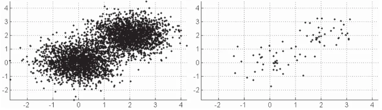
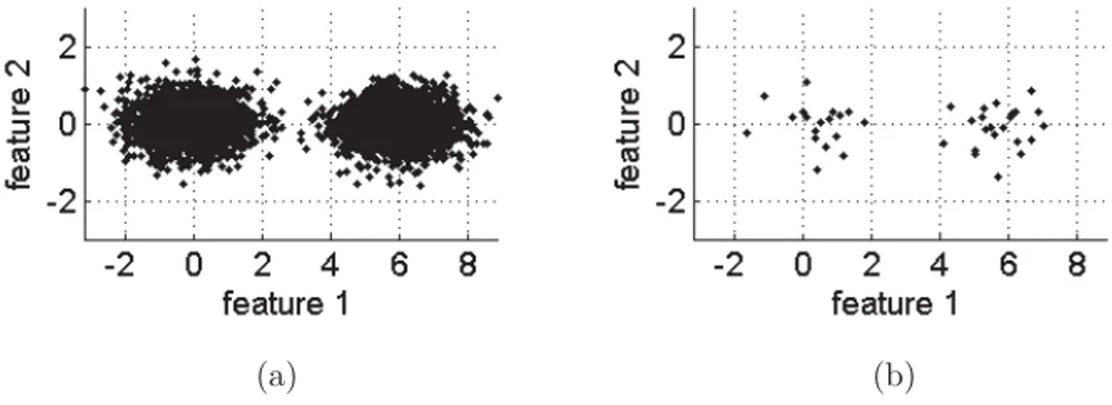
2.1 Example of data point observations distributed in bi-dimensional sub-space : the full dataset (N =4000) in the left versus a small simple random sample points (n=40) in the right. . . . 35

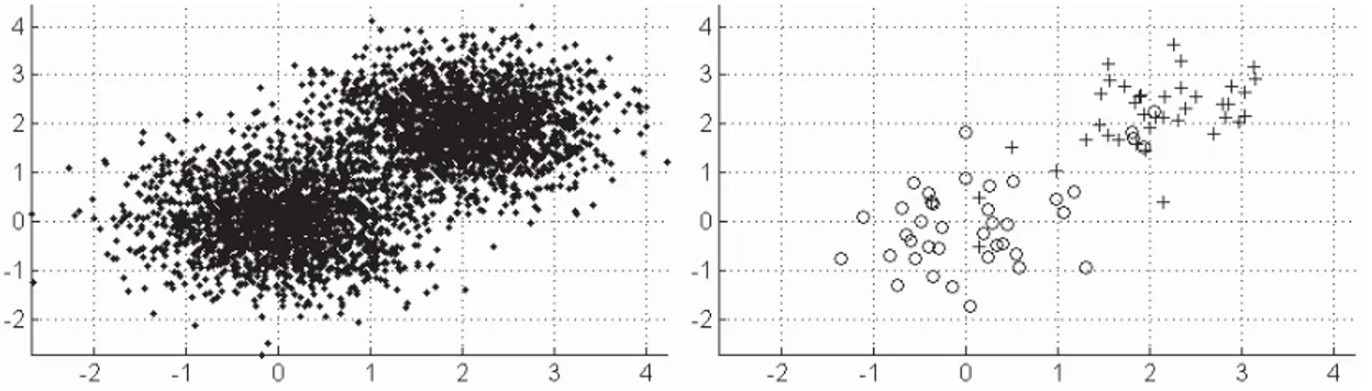
2.2 Example of data point observations distributed in bi-dimensional sub-space : the full dataset (N =4000) in the left versus a small ranked set sample points (n=40 and K=2) in the right. . . . 41

(10)

Table des figures

2.3 Dataset 1 constituted by three Gaussian distributions. First and second rows represent respectively SRS and RSS samples with its histograms. Ranked-k-means is used with α=0.2 and K=3. Red vertical lines re-present the centers of each cluster obtained by the E-step of SRS and ranked k-means.. . . 44

2.4 Dataset 2 constituted by ﬁve Gaussian distributions. First and second rows represent respectively SRS and RSS samples with its histograms. Ranked-k-means is used with α=0.4 and K=5. Red vertical lines re-present the centers of each cluster obtained by the E-step of SRS and ranked k-means.. . . 44

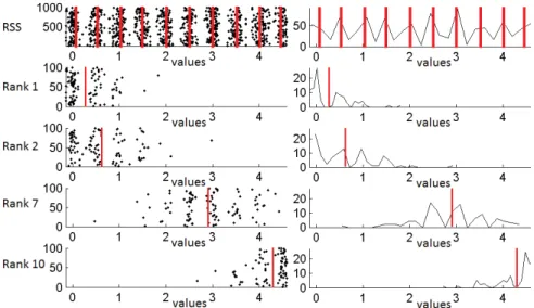
2.5 Dataset 3 constituted by ten Gaussian distributions. First and second rows represent respectively SRS and RSS samples with its histograms. Ranked-k-means is used with α=0.2 and K=10. Red vertical lines re-present the centers of each cluster obtained by the E-step of SRS and ranked k-means.. . . 45

2.6 First row represents RSS sample of dataset 1 and its histogram, and the red vertical lines represent the estimated centers ml. Below the ﬁrst row, each row represents one subpopulation of RSS and its histogram, and the red vertical lines represent the subpopulation means wk. . . . 45

2.7 First row represents RSS sample of dataset 2 and its histogram, and the red vertical lines represent the estimated centers ml. Below the ﬁrst row, each row represents one subpopulation of RSS and its his-togram (for ranks 1, 2 and 5), and the red vertical lines represent the subpopulation means wk. . . . 46

2.8 First row represents RSS sample of dataset 3 and its histogram, and the red vertical lines represent the estimated centers ml. Below the ﬁrst row, each row represents one subpopulation of RSS and its histogram (for ranks 1, 2, 7 and 10), and the red vertical lines represent the subpopulation means wk. . . . 47

2.9 Center positions obtained by our estimation approach in dataset 1 for

(11)

Table des figures

2.10 Variation of the obtained centers for each value of α (from 0 to 2) for the three datasets. The parameter K is equal respectively to 3, 5 and 10 in the left and 6, 10 and 20 in the right. The sample size n is ﬁxed to the whole dataset size N . . . . 49

2.11 Center positions obtained by our estimation approach in dataset 1 for

K = 1, K = 3 and K = 6. . . . 50

2.12 Variation of the obtained centers for each value of K (from 1 to 20). The sample size n is ﬁxed to the whole dataset size N . . . . 51

2.13 Center positions obtained by our estimation approach in dataset 1 for diﬀerent sample sizes : n=48, n=150, and n=1500. . . . 52

2.14 Variation of the obtained centers for each value of the sample size n (from 1 to N ). The subpopulation number K is ﬁxed to the center number L. . . . 53

2.15 Visible (first row) and THz (second row) images respectively of carbon fiber (first column), flexure spring (second column) and grape (third column). THz images are shown using the maximal amplitude feature. 59

2.16 Standard k-means segmentation of the three THz images : carbon fi-ber image (first column), flexure spring image (second column) and grape image (third column). The approach was used respectively with L equal to 3, 3 and 5 clusters for the three images. The AR(p)/PCA(q) extracted features were used with p=2 and q=1 for the carbon and the spring images and p=3 and q=1 for the grape image. . . . 59

2.17 Bradley segmentation of the three THz images : carbon fiber image (first row), grape image (second row) and flexure spring image (third row). The Bradley approach was used respectively with L = 3, L = 3 and L = 5, and the sample size n equal to 30 (first column), 300 (se-cond column) and 3000 (third column). The AR(p)/PCA(q) extracted features were used with p=2 and q=1 for the carbon and the spring images and p=3 and q=1 for the grape image. . . . 60

(12)

Table des figures

2.18 SRS-k-means segmentation of THz images of carbon fiber (first row), flexure spring (second row) and grape (third row). For the three images, SRS-k-means has used respectively L = 3, L = 3 and L = 5, and the sample size n equal to 30 (first colomn), 300 (second column) and 3000 (third column). The AR(p)/PCA(q) extracted features were used with p=2 and q=1 for the carbon and spring images and p=3 and q=1 for the grape image. . . 61

2.19 Ranked-k-means segmentation of THz images of carbon fiber (first row), flexure spring (second row) and grape (third row). For the three images, ranked-k-means has used respectively L = 3, L = 3 and L = 5, and the sample size n equal to 30 (first colomn), 300 (second column) and 3000 (third column). The AR(p)/PCA(q) extracted features were used with p=2 and q=1 for the carbon and spring images and p=3 and

q=1 for the grape image. . . . 62

3.1 Schematic of Terahertz imaging formation in transmission mode. (a) shows an interaction of T-rays with a sample of carbon fiber. The THz signals are projected to the sample, interacted with it and then detected to constitute the THz data cube in (b). The detected T-rays form the different regions in the sample. The obtained THz data in (b) is represented by R×C pixels and characterized by P raw features. Two pixels are colored in blue and orange which belong respectively to a typical region of the carbon fiber and a damaged zone. (c) contains two different THz responses colored in blue and orange which correspond respectively to the two pixels in the Terahertz image in (b) with the same color. . . 71

3.2 Example of data point observations distributed in bi-dimensional sub-space : (a) the full dataset X (N = 4000) versus (b) a small simple random sample points XSRS (n = 40). . . . 78

(13)

Table des figures

3.3 (a) The within-cluster dispersion ϕp and (b) the ﬁnal feature weights wp obtained as output of W-k-means clustering on the dataset X shown in ﬁgure 3.2 (a). The ϕp and the wp are shown inversely proportional for the two features of the dataset X. . . . 78

3.4 (a) SRS sample (XSRS) of n = 40 points. The SS-k-means clustering of XSRS gives the within-cluster dispersion ϕp and the global-data disper-sion ψp shown respectively in (b) and (c). (d), (e), (f) and (g) represent the ﬁnal feature weights for c equal to 0, 0.5, 1 and 2. . . . 82

3.5 The ﬁnal feature weights of SS-k-means on the synthetic dataset 1 for

c equal to (a) 0, (b) 0.5, (c) 1, (d) 1.5, (e) 2, (f) 2.5, and (g) 3. . . . . 85

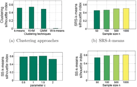
3.8 Variation of the clustering performance provided by SS-k-means for diﬀerent values of c on (a) synthetic dataset 1, (b) synthetic dataset 2 and (c) synthetic dataset 3. . . 88

3.9 Variation of the Silhouette cluster validity index provided by SS-k-means for diﬀerent values of c on (a) synthetic dataset 1, (b) synthetic dataset 2 and (c) synthetic dataset 3. . . 88

3.10 An image of four chemical compounds acquired in visible spectrum in the left and the ground truth of the Terahertz image in the right. The false colors red, blue, green and yellow correspond respectively to the chemical compounds L-Tryptophan (0.200g), L-Tryptophan (0.100g), L-Valine (0.200g) and Proline (0.200g). . . 89

3.11 An image of a moth acquired in visible spectrum in the left and the 570th _{band of the THz image in the right.} _{. . . .} ₈₉ 3.12 An aluminum substrate with diﬀerent thickness is acquired in the

vi-sible light. The image contains a letter "H" primed in the left and pain-ted in the middle. The 680th _{band of the paint THz image is shown in} the right.. . . 90

(14)

Table des figures

3.13 Three curves of the silhouette index measurements of SS-k-means on the chemical THz image. The ﬁrst curve is a function of a (b = 2 and c = 1.2), the second curve is a function of b (a = 2 and c = 1.2), and the third curve is a function of c (a = 2 and b = 2). . . . 90

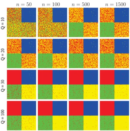
3.14 SRS-k-means segmentation of the chemical THz image for diﬀerent values of the sample size n.. . . 91

3.15 Chemical THz image segmentation for k-means (a), KHM (b), GMM (c), W-k-means (d) and SS-k-means for c equal to 0.5 (e), 1 (f), 1.2 (g), 1.5 (h), 2 (i), and 2.5 (j). . . 91

3.16 (a) Initial random feature weights. Final feature weights of W-k-means (b) and SS-k-means on the chemical THz image for c equal to 0.5 (c), 1 (d), 1.2 (e), 1.5 (f), 2 (g), and 2.5 (h).. . . 92

3.17 Clustering performances on the chemical THz image for (a) k-means, KHM, GMM, W-k-means, (b) SRS-k-means, (c) SS-k-means for c = 0.5, 1, 1.2, 1.5, 2, and 2.5 (n = N and Q = P ) and (d) SS-k-means for

n = 50, 100, 500, 1000 and 1500 (c = 1.2 and Q = 30). . . . 93

3.18 Silhouette index of the chemical THz image segmentation obtained by (a) k-means, KHM, GMM, W-k-means, (b) SRS-k-means, (c) SS-k-means for c = 0.5, 1, 1.2, 1.5, 2, and 2.5 (n = N and Q = P ) and (d) SS-k-means for n = 50, 100, 500, 1000 and 1500 (c = 1.2 and Q = 30). 94

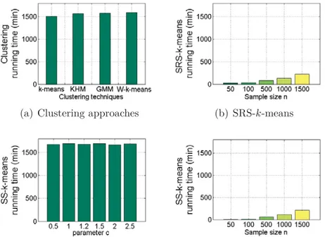
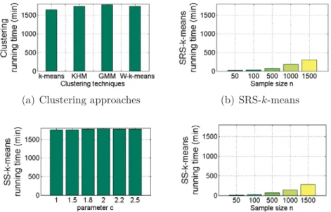
3.19 Running time of the chemical THz image segmentation using (a) k-means, KHM, GMM, W-k-k-means, (b) SRS-k-k-means, (c) SS-k-means for c = 0.5, 1, 1.2, 1.5, 2, and 2.5 (n = N and Q = P ) and (d) SS-k-means for n = 50, 100, 500, 1000 and 1500 (c = 1.2 and Q = 30). . . 95

3.20 SRS-k-means segmentation of the moth THz image for diﬀerent values of the sample size n. . . . 96

3.21 Moth THz image segmentation for k-means (a), KHM (b), GMM (c), W-k-means (d) and SS-k-means for c equal to 1 (e), 1.5 (f), 2 (g), and 2.5 (h).. . . 96

3.22 (a) Initial random feature weights. Final feature weights of W-k-means (b) and SS-k-means on the moth THz image for c equal to 1 (c), 1.5 (d), 2 (e), and 2.5 (f).. . . 97

(15)

Table des figures

3.23 Silhouette index of the moth THz image segmentation obtained by (a) k-means, KHM, GMM, W-k-means, (b) SRS-k-means, (c) SS-k-means for c = 1, 1.5, 1.8, 2, 2.2 and 2.5 (n = N and Q = P ) and (d) SS-k-means for n = 50, 100, 500, 1000 and 1500 (c = 2 and Q = 5). . . . . 98

3.24 Running time of the moth THz image segmentation using (a) k-means, KHM, GMM, W-k-means, (b) SRS-k-means, (c) SS-k-means for c = 1, 1.5, 1.8, 2, 2.2 and 2.5 (n = N and Q = P ) and (d) SS-k-means for

n = 50, 100, 500, 1000 and 1500 (c = 2 and Q = 5). . . . 99

3.25 SRS-k-means segmentation of the paint THz image for diﬀerent values of the sample size n. . . . 100

3.26 The paint THz image segmentation for k-means (a), KHM (b), GMM (c), W-k-means (d) and SS-k-means for c equal to 0.5 (e), 1 (f), 1.5 (g) and 2 (h). . . 100

3.27 (a) Initial random feature weights. Final feature weights of W-k-means (b) and SS-k-means on the paint THz image for c equal to 0.5 (c), 1 (d), 1.5 (e) and 2 (f). . . 101

3.28 Silhouette index of the paint THz image segmentation obtained by (a) k-means, KHM, GMM, W-k-means, (b) SRS-k-means, (c) SS-k-means for c = 0.5, 1, 1.5 and 2 (n = N and Q = P ) and (d) SS-k-means for

n = 50, 100, 500 and 1000 (c = 1.5 and Q = 100). . . . 102

3.29 Running time of the paint THz image segmentation using (a) k-means, KHM, GMM, W-k-means, (b) SRS-k-means, (c) SS-k-means for c = 0.5, 1, 1.5 and 2 (n = N and Q = P ) and (d) SS-k-means for n = 50, 100, 500 and 1000 (c = 1.5 and Q = 100).. . . 103

3.30 The chemical THz image segmentation of SS-k-means for diﬀerent va-lues of n and Q. . . . 104

3.31 Clustering performances, Silhouette index, and running time of SS-k-means on the chemical THz image for diﬀerent values of n and Q. . . 105

3.32 The moth THz image segmentation of SS-k-means for diﬀerent values of n and Q. . . . 106

3.33 Silhouette index and running time of SS-k-means on the moth THz image for diﬀerent values of n and Q. . . . 106

(16)

Table des figures

3.34 The paint THz image segmentation of SS-k-means for diﬀerent values of n and Q. . . . 107

3.35 Silhouette index and running time of SS-k-means on the paint THz image for diﬀerent values of n and Q. . . . 108

3.36 Variation of the precision of diﬀerent sample sizes for chemical, moth and paint Terahertz images. . . 109

4.1 Accuracy of clustering algorithms on dataset D2. The parameter K is

ﬁxed to 2. . . 123

4.2 Precision of clustering algorithms on dataset D2. The parameter K is

ﬁxed to 2. . . 123

4.3 Recall of clustering algorithms on dataset D2. The parameter K is

ﬁxed to 2. . . 124

ﬁxed to 5. . . 124

ﬁxed to 5. . . 125

ﬁxed to 3. . . 126

ﬁxed to 3. . . 127

4.10 The variation of clustering accuracy in terms of error variance σ2

n for data sets D2 (a), D3 (b) and D5 (c). Each data set was generated for

diﬀerent values of σ2

n from 10−4 to 1.2. The parameter K is ﬁxed to 2, 5 and 3 for data sets D2, D3 and D5. . . 128

4.11 MGIC criterion for data set D2. MGIC(P ,K,α) is presented for

dif-ferent values of K from 2 to 10 (from the left to the right and from the top to the bottom) and P from 1 to 10. The parameter α is ﬁxed to 2. 129

(17)

Table des figures

dif-ferent values of K from 2 to 10 (from the left to the right and from the top to the bottom) and P from 1 to 10. The parameter α is ﬁxed to 2(log(log(T + N ))). . . . 130

4.17 In the left, an image of four chemical compounds acquired in visible spectrum. In the right, the ground truth of the THz image. The false co-lors green, blue, red and yellow correspond respectively to the chemical compounds L-Valine (0.200g), L-Tryptophan (0.100g), L-Tryptophan (0.200g) and Proline (0.200g). . . 135

4.18 In the left and the middle, an image of a cork acquired in visible spec-trum. In the right, the 195th _{band of the THz image.} _{. . . 135} 4.19 In the left, an image of a moth acquired in visible spectrum. In the

right, the 570th _{band of the THz image.} _{. . . 135} 4.20 Chemical THz image segmentation for K-means (a), KHM (b), GMM

(c), W-K-means (d), SS-K-means for c = 0.5 (e), c = 1 (f) and c = 2.5 (g), AC+K-Means for L = 5 (h), L = 10 (i), AR+K-Means for P = 5 (j), P = 10 (k), and K-AR for P = 2 (l), P = 5 (m), P = 10 (n),

(18)

Table des figures

4.21 Accuracy of the clustering algorithms on chemical THz image. . . 137

4.22 Precision of the clustering algorithms on chemical THz image. . . 137

4.23 Recall of the clustering algorithms on chemical THz image. . . 138

4.24 Cork THz image segmentation for K-means (a), KHM (b), GMM (c), W-K-means (d), SS-K-means for c = 0.5 (e), c = 1 (f) and c = 2 (g), AC+K-Means for L = 8 (h), L = 10 (i), AR+K-Means for P = 8 (j), P = 10 (k), and K-AR for P = 1 (l), P = 4 (m), P = 8 (n), P = 10 (o) and P = 12 (p). . . . 139

4.25 Moth THz image segmentation for K-means (a), KHM (b), GMM (c), W-K-means (d), SS-K-means for c = 1 (e), c = 1.5 (f) and c = 2 (g), AC+K-Means for L = 3 (h), L = 6 (i), AR+K-Means for P = 3 (j), P = 6 (k), and K-AR for P = 2 (l), P = 3 (m), P = 4 (n), P = 6 (o) and P = 10 (p). . . . 140

4.26 Modiﬁed generalized information criterion (MGIC) computed after the chemical THz image segmentation for diﬀerent values of parameters P and K. . . . 141

4.27 Modiﬁed generalized information criterion (MGIC) computed after the cork THz image segmentation for diﬀerent values of parameters P and

K. . . . 141

4.28 Modiﬁed generalized information criterion (MGIC) computed after the moth THz image segmentation for diﬀerent values of parameters P and

K. . . . 142

5.1 Clustering performances on dataset D2 for K-means, KHM, GMM,

W-K-means and SS-K-means (in the left) and MoAR for P from 1 to 10 (in the right). The parameter K is ﬁxed to 2. . . . 155

(19)

Table des figures

5.4 MGIC criterion for dataset D2. MGIC(P ,K,α) is presented for diﬀerent

values of K and P . The parameter α is ﬁxed to 2. . . . 158

values of K and P . The parameter α is ﬁxed to 2 ln ln(T N ). . . . 158

5.10 Clustering performances on the TRACE dataset for K-means, KHM, GMM, W-K-means and SS-K-means (in the left) and MoAR for P from 1 to 10 (in the right). The parameter K is ﬁxed to 4. . . . 162

5.11 MGIC criterion for TRACE dataset. MGIC(P ,K,α) is presented for diﬀerent values of K and P . The parameter α is ﬁxed to 2. . . . 163

5.12 MGIC criterion for TRACE dataset. MGIC(P ,K,α) is presented for diﬀerent values of K and P . The parameter α is ﬁxed to 2 ln ln(T N ). 163

5.13 Two time series from the RobotSurface dataset. Solid and dashed lines correspond to the robot walking respectively on carpet and cemented surfaces. . . 164

5.14 Clustering performances on RobotSurface dataset for K-means, KHM, GMM, W-K-means and SS-K-means (in the left) and MoAR for P from 1 to 10 (in the right). The parameter K is ﬁxed to 2. . . . 165

5.15 MGIC criterion for RobotSurface dataset. MGIC(P ,K,α) is presented for diﬀerent values of K and P . The parameter α is ﬁxed to 2. . . . . 166

5.16 MGIC criterion for RobotSurface dataset. MGIC(P ,K,α) is presented for diﬀerent values of K and P . The parameter α is ﬁxed to 2 ln ln(T N ).166

(20)

Table des figures

5.17 In the left, an image of four chemical compounds acquired in visible spectrum. In the right, the ground truth of the THz image. The false co-lors green, blue, red and yellow correspond respectively to the chemical compounds L-Valine (0.200g), L-Tryptophan (0.100g), L-Tryptophan (0.200g) and Proline (0.200g). . . 167

5.18 In the left, an image of four chemical compounds acquired in visible spectrum. In the right, the ground truth of the THz image. The false colors blue, orange, purple and grey correspond respectively to the chemical compounds L-Lystine (0.200g), DL-Asperic Acid (0.200g) + PE Powder (0.100g), BSA (0.075g)+ PE Powder (0.125g) and BSA (0.155g). . . 167

5.19 (a) Front and (b) back images of a cork acquired in visible spectrum. (c) The 195th _{band of the THz image. (d) The 195}th _{band of a higher} resolution THz image of the portion outlined in red. . . 168

5.20 Chemical THz image 1 segmentation for K-means (a), KHM (b), GMM (c), W-K-means (d), SS-K-means for c = 0.5 (e), c = 1 (f) and c = 2.5 (g), and MoAR for P = 5 (h), P = 8 (i), P = 10 (j), P = 16 (k) and

P = 20 (l). . . . 169

5.21 Clustering performances on chemical THz image 1 for K-means, KHM, GMM and W-K-means (in the left), SS-K-means for diﬀerent values of c (in the middle), and MoAR for divers values of P (in the right). . 170

5.22 Chemical THz image 2 segmentation for K-means (a), KHM (b), GMM (c), W-K-means (d), SS-K-means for c = 0.5 (e), c = 1 (f) and c = 1.5 (g), and MoAR for P = 3 (h), P = 5 (i), P = 7 (j), P = 8 (k) and

P = 10 (l). . . . 171

5.23 Clustering performances on chemical THz image 2 for K-means, KHM, GMM and W-K-means (in the left), SS-K-means for diﬀerent values of c (in the middle), and MoAR for divers values of P (in the right). . 172

5.24 Cork THz image 1 segmentation for K-means (a), KHM (b), GMM (c), W-K-means (d), SS-K-means for c = 0.5 (e), c = 1 (f) and c = 2 (g), and MoAR for P = 1 (h), 3 (i), 7 (j), 11 (k) and 15 (l).. . . 173

(21)

Table des figures

5.25 Cork THz image 2 segmentation for K-means (a), KHM (b), GMM (c), W-K-means (d), SS-K-means for c = 0.5 (e), c = 1 (f) and c = 2 (g), and MoAR for P = 1 (h), 5 (i), 10 (j), 12 (k) and 15 (l). . . . 174

5.26 Modiﬁed generalized information criterion (MGIC) computed after the chemical THz image 1 segmentation for diﬀerent values of parameters

P and K. . . . 175

5.27 Modiﬁed generalized information criterion (MGIC) computed after the chemical THz image 2 segmentation for diﬀerent values of parameters

P and K. . . . 175

5.28 Modiﬁed generalized information criterion (MGIC) computed after the cork THz image 1 segmentation for diﬀerent values of parameters P and K. . . . 176

5.29 Modiﬁed generalized information criterion (MGIC) computed after the cork THz image 2 segmentation for diﬀerent values of parameters P and K. . . . 176

(22)

Liste des tableaux

1 Résumé des principaux avantages et inconvénients de l’imagerie avec les radiations (rayons) Térahertz par rapport aux autres technologies. Tableau extrait de [95] . . . 18

1.1 Résumé de quelques travaux sur la segmentation d’images Térahertz . 27

2.1 Summary of some related works on Terahertz image segmentation . . 33

2.2 Clustering performances, centers accuracies and cluster validity indices of dataset 1 . . . 55

2.5 Clustering performances, centers accuracies and cluster validity indices of Iris dataset . . . 56

2.6 Clustering performances, centers accuracies and cluster validity indices of Yeast dataset . . . 57

2.7 Centers accuracies and cluster validity indices of the Terahertz carbon ﬁber image. . . 64

2.8 Centers accuracies and cluster validity indices of the Terahertz grape image . . . 64

2.9 Centers accuracies and cluster validity indices of the Terahertz ﬂexure spring image . . . 65

(23)

Liste des tableaux

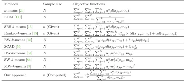
3.1 Summary of some related works on k-means clustering techniques in terms of sample size and objective function. d(xjp, mlp) is the Euclidian distance between xjp and mlp. ujl is the membership degree of the jth data point to the lth _{cluster. mlp} _{is the l}th _{center for the p}th _feature. wp is the pth _{feature weight.} _{. . . .} ₇₄ 3.2 Summary of some related works on k-means clustering techniques in

terms of membership degrees, centers and feature weights. d(xjp, mlp) is the Euclidian distance between xjp and mlp. ujl is the membership degree of the jth _{data point to the l}th _{cluster. mlp} _{is the l}th _{center for} the pth feature. wp is the pth feature weight. . . 75

(24)

Introduction

Le présent chapitre introduit la technologie d’imagerie avec les radiations Téra-hertz. Il présente ensuite le processus de formation de cette technologie d’images et énumère les motivations pour analyser les images Térahertz. Ce chapitre décrit la feuille de route pour notre thèse et un bref résumé des contributions présentées dans notre travail.

1 Radiation et imagerie Térahertz

Au cours des dernières années, des nombreux groupes de recherche à travers le monde sont intéressés à la portion Térahertz (THz) des rayonnements

électromagné-tiques [33,42,63,112]. Les rayonnements Térahertz (rayons T) se réfèrent à la région

du rayonnement électromagnétique occupant la bande de fréquences de 0.1 à 10 THz (qui correspond à des longueurs d’ondes comprises entre 3 mm et 3 μm), délimitées

par les micro-ondes et les ondes infrarouges (voir la ﬁgure1). Par rapport aux régions

optiques, infrarouges et rayons X, les développements technologiques avancés dans la région Térahertz sont limités. Cependant, les progrès récents dans les technologies électro-optiques rendent actuellement la région Térahertz disponible pour un usage pratique. Ces progrès technologiques ont rendu possible la génération et la détection des rayons T avec des dispositifs eﬃcaces. Une portion inutilisée du spectre électroma-gnétique devient disponible, c’est une portion d’un grand potentiel pour la détection

et l’imagerie en microélectronique [6, 5, 63], en diagnostic médical [54, 55, 85, 112],

en contrôle environnemental [33, 83, 82], en sécurité [101, 71, 76], en identiﬁcation

chimique et biologique [113, 52,102], en contrôle de qualité [14, 82,58, 59], etc.

(25)

1. Radiation et imagerie Térahertz

ﬁgure 1 – Spectre des ondes électromagnétiques. Les ondes Térahertz sont déﬁnies entre les micro-ondes et les ondes infrarouge.

des applications scientiﬁques et industrielles [42, 54, 82, 83, 99, 90, 66, 60]. Bien

que d’autres portions électromagnétiques sont assez utilisées dans des applications de l’imagerie numériques, les propriétés de l’imagerie avec les rayonnements

Téra-hertz leurs permettent d’occuper une position importante. Le tableau 1 résume les

principaux avantages et inconvénients de l’imagerie avec les rayons T par rapport aux autres technologies, telles que les micro-ondes, les infrarouges et les rayons X. Les micro-ondes offrent une bonne profondeur de pénétration à travers des objets opaques, mais ils permettent une faible résolution spatiale. Les rayonnements infra-rouges offrent une bonne résolution spatiale, mais ils permettent une faible profondeur de pénétration à travers les objets opaques. Les rayons X offrent la meilleure résolution spatiale et la profondeur de pénétration la plus élevée, mais ils sont potentiellement invasifs pour les organismes vivants ou les tissus biologiques inspectés. L’imagerie avec les rayons T offre un bon compromis entre les modalités mentionnées ci-dessus. Les rayons T sont moins énergétiques que les rayons X et ne semblent pas présenter aucun risque de santé pour l’inspection des organismes vivants, des tissus biologiques, des

nourritures et textiles industriels [23]. Les rayons Térahertz produisent des

(26)

1. Radiation et imagerie Térahertz

Radiations Avantages Inconvénients

- Pas dangereuses - Faible résolution spatiale

Micro- - Bonne pénétration dans des nombreux - Les métaux et l’eau bloquent le

rayon-ondes matériaux nement

- Système d’acquisition d’images rapide - Imagerie spectrale non disponible - Coût élevé de maintenance - Pas dangereuses - Faible profondeur de pénétration Infra- - Bonne résolution spatiale - Imagerie spectrale non disponible rouges - Système d’acquisition d’images rapide

- Coût acceptable de maintenance

- Haute profondeur de pénétration - Dangereuses pour les êtres vivants Rayons X - Excellente résolution spatiale - Coût élevé de maintenance

- Système d’acquisition d’images rapide - Imagerie spectrale non disponible - Pas dangereuses - Système d’acquisition d’images lent Rayons T - Bonne profondeur de pénétration - Les métaux et l’eau bloquent le

rayon-- Bonne résolution spatiale nement

- Imagerie spectrale disponible - Coût élevé de maintenance

tableau 1 – Résumé des principaux avantages et inconvénients de l’imagerie avec les radiations (rayons) Térahertz par rapport aux autres technologies. Tableau extrait de

[95]

la discrimination des matériaux spéciﬁques à l’intérieur d’un objet. Par rapport aux micro-ondes, les courtes longueurs d’onde de la portion Térahertz permettent une plus grande résolution spatiale. En résumé, les rayons Térahertz sont caractérisés par plu-sieurs propriétés importantes, parmi lesquelles, l’inspection non invasive des objets, la pénétration à travers des objets secs et non métalliques tels que le plastique, le carton,

le bois et le tissu et offrent une identification spécifique des matériaux [54,19, 23].

Cependant, par rapport aux modalités d’imagerie bien développées, comme les in-frarouges et les rayons X, les systèmes d’acquisition d’images THz ont des dispositifs d’acquisition lents. Cette lenteur s’explique par l’immaturité de cette nouvelle moda-lité. Dans ce qui suit, nous présentons le processus de formation d’images Térahertz, suivi par d’autres déﬁs rencontrés par cette technologie d’images et les motivations pour son analyse et son interprétation.

(27)

2. Formation d’images Térahertz

2 Formation d’images Térahertz

L’imagerie avec les rayons Térahertz peut être obtenue par une acquisition en deux modes passif ou actif. Un système passif utilise la lumière du soleil comme une source et détecte les rayons Térahertz émis naturellement par un objet. Le système actif diffère du système passif par l’utilisation d’une source active des rayons THz artificiels pour éclairer l’objet et détecter les rayons THz transmis ou réfléchis. Dans notre travail, les acquisitions sont utilisées uniquement en mode actif.

Il y a presque quarante ans, la génération des radiations électromagnétiques est

apparue en utilisant le laser à impulsions ultra-brèves [11]. Les impulsions laser

fem-toseconde sont utilisées pour générer des impulsions électriques picosecondes dont les bandes spectrales se trouvent dans la région Térahertz. La spectroscopie Térahertz dans le domaine temporel est d’abord utilisée pour détecter ces impulsions à large

bande aﬁn d’analyser la réponse spectrale des matériaux [114]. Cette technique est

ensuite étendue à l’imagerie Térahertz, qui peut être mise en oeuvre en mode de ré-ﬂexion ou de transmission. Dans la suite de ce chapitre, nous décrivons un système

d’acquisition de l’image THz en mode transmission (voir ﬁgure2). Le système

d’acqui-sition enregistre les réponses spectroscopiques d’un échantillon qui est cartographié

à plusieurs positions contigus de pixels [63]. Le système d’acquisition d’images

Té-rahertz commence par émettre des impulsions laser ultra-rapide (typiquement entre 10 et 100 fs) vers un séparateur de faisceaux. Les impulsions laser sont divisées en faisceaux de pompe et de sonde. Le faisceau de pompe est utilisé pour générer des rayons Térahertz et le faisceau de sonde est utilisé pour détecter le champ électrique des rayons THz d’une manière cohérente. Les rayons Térahertz à large bande sont gé-nérés par l’illumination avec le faisceau de pompe dans un cristal (tel que ZnTe, GaAs

et InP) avec rectiﬁcation optique [54]. Des miroirs paraboliques sont nécessaires pour

focaliser les rayons Térahertz produits vers un endroit où l’échantillon est situé. Les rayons Térahertz interagissent avec l’échantillon avant d’être transmis au détecteur au moyen de miroirs paraboliques. À un instant donné, le détecteur est déclenché par le faisceau de sonde et l’amplitude du champ électrique Térahertz est mesurée. L’instant de la mesure est déterminé par le retard du faisceau de sonde. Le balayage de toute l’impulsion Térahertz par la ligne à retard du faisceau de sonde permet de reconstruire

(28)

2. Formation d’images Térahertz

ﬁgure 2 – Schéma typique d’un système de formation d’images Térahertz en mode

transmission (ﬁgure extraite de [54]). Les signaux THz sont projetés sur l’objet,

inter-agis avec celui-ci, puis détectés pour constituer un cube de données THz. Les signaux projetés sont similaires, tandis que les signaux détectés sont modiﬁés qui illustrent les diﬀérentes régions de l’objet.

cette impulsion en une série de points discrets [54]. L’ensemble d’impulsions détectées

sont alors enregistrées à plusieurs emplacements contigus qui constituent les pixels de l’image THz. Chaque pixel est considéré comme une série chronologique représentée par plusieurs bandes, caractéristiques ou attributs (par exemple, 1500 bandes). Ainsi, la combinaison de ces séries en lignes et en colonnes constitue un cube de données

Térahertz brutes (par exemple, le cube R× C × P dans la ﬁgure 3, où R, C et P

représentent respectivement le nombre de lignes, de colonnes et de bandes). Pour visualiser l’image THz, les caractéristiques peuvent être extraites pour créer l’image 2D. On peut sélectionner l’amplitude pour un délai de temps spéciﬁque, l’amplitude

(29)

3. Problématique de la thèse

(a) Cube 3D de données THz (b) Deux réponses (signaux) Térahertz

ﬁgure 3 – (a) Cube 3D de données Térahertz représenté par R×C pixels et caractérisé

par des P attributs brutes. Deux pixels colorés en bleu et en orangé appartiennent respectivement à une région typique de la ﬁbre de carbone et à une région endom-magée. (b) contient deux réponses THz diﬀérentes colorées en bleu et en orangé qui correspondent respectivement aux deux pixels de l’image Térahertz en (a) pour la même couleur.

maximale ou minimale de chaque série ou l’amplitude de la transformée de Fourier

prise sur un intervalle de temps [54,22].

3 Problématique de la thèse

L’imagerie dans le domaine Térahertz peut fournir des informations temporelles et spectrales spéciﬁques et non disponibles pour d’autres modalités. Cependant, l’ima-gerie Térahertz fait face à des déﬁs pour pouvoir l’analyser et l’interpréter auto-matiquement. La quantité énorme de caractéristiques brutes peut être un obstacle pour décrire avec une certaine précision le contenu informationnel des images THz

[112, 85, 51]. De plus, certaines caractéristiques de l’image THz brute peuvent être

bruitées, redondantes ou non informatives [14]. Le nombre élevé de pixels peut aussi

être une barrière pour analyser ce type d’images [61,15]. Le traitement de l’ensemble

(30)

4. Contributions

L’objectif de cette thèse est de segmenter les images Térahertz en utilisant des mé-thodes d’analyse de données. La segmentation de ces images consiste à partitionner l’ensemble de pixels en plusieurs régions homogènes pour localiser des objets dans les images. Ces objets sont supposés disjoints et les régions qui les constituent, forment des classes séparées dans l’espace de caractéristiques. Vue la quantité énorme de ca-ractéristiques, nous proposons dans cette thèse des stratégies de réduction de l’espace de caractéristiques. L’extraction de caractéristiques et la reconnaissance d’objets sont eﬀectuées dans l’espace réduit. Pour ce faire, nous privilégierons d’utiliser des tech-niques de classiﬁcation pour analyser ce type d’images. Dans la section suivante, nous présentons nos contributions relatives à l’analyse d’images Térahertz.

4 Contributions

Les deux premiers chapitres introduisent deux nouvelles approches de segmenta-tion basées sur des techniques d’échantillonnage. Dans la première approche, nous formulons la technique de classiﬁcation K-means dans le cadre de l’échantillon d’en-sembles ordonnés pour surmonter le problème d’initialisation des centres. Le deuxième chapitre aborde la sélection des données à travers la pondération de caractéristiques et l’échantillonnage aléatoire simple pour la classiﬁcation des pixels en vue d’une segmen-tation des images Térahertz. Une estimation automatique de la taille de l’échantillon aléatoire et du nombre de caractéristiques sélectionnées sont également proposés. Dans ces deux chapitres, nous avons réalisé des tests sur des ensembles de données de synthèse et d’images Térahertz qui ont permis d’évaluer la performance des méthodes proposées par rapport à l’état de l’art.

Les deux derniers chapitres introduisent une autre famille de techniques de clas-sification des pixels basées sur la régression et qui sont adaptées aux séries chronolo-giques. Nous supposons que les valeurs associées à chaque pixel d’une image Térahertz sont échantillonnées à partir d’un modèle autorégressif. La segmentation de l’image est alors vue comme un problème de classification de séries chronologiques. Ainsi, dans le troisième chapitre, la classification est formulée comme un problème d’optimisation non-linéaire. L’ordre du modèle et le nombre de classes sont estimés en utilisant un cri-tère généralisé d’information. Finalement, le quatrième chapitre est une généralisation

(31)

4. Contributions

des résultats obtenus dans le troisième chapitre. Au lieu de considérer un problème de moindres carrés, nous proposons une approche de classiﬁcation probabiliste basée sur le mélange de modèles autorégressifs. Les paramètres de l’approche proposée sont estimés en utilisant un critère généralisé d’information. Les résultats expérimentaux montrent que l’approche proposée permet de segmenter des images Térahertz avec plus de précision que d’autres approches de l’état de l’art. L’approche proposée est utilisée aussi pour détecter la nature de la surface d’un robot mobile et discriminer des événements transitoires pour assurer un fonctionnement sûr et économique du processus de surveillance.

(32)

Chapitre 1

État de l’art

1 Introduction

L’interaction du rayonnement Térahertz avec l’objet à analyser peut être définie en traitant l’ensemble de matériaux qu’ils constituent. Ces matériaux doivent avoir des réponses dans le domaine THz pour dire que les différentes structures de l’objet sont plus ou moins transmissibles ou réfléchissantes, afin de pouvoir les discriminer. L’eau et les objets humides absorbent fortement les radiations THz ; toutefois, les objets secs (tels que le papier, le tissu, le plastique et le bois) sont transparents aux radiations THz et ne fournissent pas de radiations réfléchies significatives. Les métaux sont opaques aux radiations Térahertz et reflètent la plupart des radiations entrantes. D’autres matériaux intéressants, qui offrent des radiations THz spécifiques,

sont détaillés dans [54,21].

Grace aux propriétés intéressantes des rayonnements Térahertz, plusieurs travaux d’imagerie Térahertz ont été proposés dans la littérature. Dans les travaux de Kamba

et al. [69], l’imagerie Térahertz a été utilisée pour inspecter la structure des couches

internes de la monture en bois sur un tableau de peinture Japonais avant sa

res-tauration. Bowen et al. [26] ont proposé un certain nombre de techniques qui ont

été utilisées pour faciliter la récupération d’images Térahertz ﬁables à partir d’objets complexes appartenant au domaine du patrimoine culturel. Ces techniques tentent de

(33)

2. Travaux connexes sur la segmentation d’images Térahertz

surmonter les problèmes posés par les surfaces inégales, en améliorant la résolution en profondeur et le contraste de l’image. Dans le domaine de la sécurité, Kowalski et

al. [71] ont proposé une application qui consiste à détecter et à visualiser des objets

cachés. Les propriétés des rayons THz et visibles sont exploitées et la combinaison des images fournies par les deux types de caméras permet de découvrir des objets dange-reux cachés à l’intérieur des vêtements. Un certain nombre de traitements d’images Térahertz existent en littérature comprenant le débruitage d’impulsions THz, l’ex-traction de bandes pertinentes et la segmentation par classiﬁcation de pixels THz, etc. En fait, il est connu que les systèmes d’imagerie Térahertz produisent des impul-sions bruitées à cause des erreurs à la fois systématiques et aléatoires. Handley et al.

[61] proposent une première méthode permettant de réduire les erreurs aléatoires. Ce

travail modélise et extrait le bruit inclus dans les impulsions des images Térahertz.

Ferguson [51] a proposé deux techniques principales de prétraitement : le débruitage

par ondelettes et la déconvolution de Wiener. Ces méthodes ont été étudiées expé-rimentalement et ses performances ont été quantiﬁées avant de segmenter l’image Térahertz.

2 Travaux connexes sur la segmentation d’images

Térahertz

L’image Térahertz est décrit par un nombre énorme de caractéristiques. La haute dimensionnalité des images Térahertz pose de nouveaux déﬁs pour la détection de

ca-ractéristiques pertinentes. Le tableau 1.1 présente un résumé de plusieurs méthodes

de segmentation d’images Térahertz. Certains travaux sont résumés dans cette section en termes d’espace de caractéristiques utilisées et de techniques de classiﬁcation su-pervisées ou non susu-pervisées. L’espace de base est constitué par les vecteurs complets

dans le domaine temporel représentant les pixels de l’image Térahertz [21]. Les autres

espaces de caractéristiques sont obtenus en utilisant des transformations de Fourier

ou d’ondelettes [101,110,109]. Ces espaces peuvent être utilisés avec une seule bande

ou avec plusieurs bandes. Dans le premier cas, le choix de la bande peut être ﬁxé à

(34)

de la forme des vecteurs représentant les pixels dans le domaine temporel ou

spec-tral sont utilisées, telles que l’amplitude du pic maximal du vecteur [50,22]. Dans le

deuxième cas, plusieurs bandes sont utilisées, telles que le vecteur entier de l’image Térahertz, l’amplitude spectrale complète et une collection de bandes de l’image THz

[50, 110, 22, 21]. Certains auteurs proposent de réduire l’espace disponible en

utili-sant les modèles autorégressifs, les modèles autorégressifs et moyennes mobiles,

l’ana-lyse en composantes principales et l’arbre de décision [50, 109, 113, 14, 31, 85]. La

segmentation des images Térahertz est généralement réalisée en termes de classiﬁca-tion supervisée, telles que le classiﬁcateur Mahalanobis, SVM et réseaux de neurones

[50,110,109,113], et de classiﬁcation non supervisée, telles que K-means, ISODATA,

hiérarchique et KHM [101,14,15,22,21,31,85]. Dans la section suivante, nous

pré-sentons nos contributions relatives à l’analyse d’images Térahertz.

Parmi les récents travaux, Holzinger et al. [72] ont proposé une approche de

clas-siﬁcation k plus proches voisins pour segmenter les mesures Térahertz de la structure interne des dents contenant des caries. Les résultats de segmentation montrent les

ré-gions qui representent les structures internes en couches des dents. Siuly et al. [100] ont

proposé une méthode d’apprentissage automatique pour la classiﬁcation des images Térahertz dans le domaine biomédical. Des fonctions de corrélation croisée 2D, des méthodes d’extraction de caractéristiques statistiques et de classiﬁcation standards sont utilisées ensemble pour analyser les images THz. Une étude des récents travaux

(35)

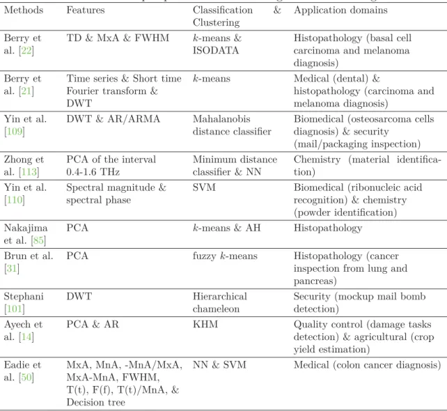
tableau 1.1 – Résumé de quelques travaux sur la segmentation d’images Térahertz

Methods Features Classiﬁcation & Clustering

Application domains Berry et

al. [22]

TD & MxA & FWHM k-means & ISODATA

Histopathology (basal cell carcinoma and melanoma diagnosis)

Berry et al. [21]

Time series & Short time Fourier transform & DWT

k-means Medical (dental) &

histopathology (carcinoma and melanoma diagnosis)

Yin et al. [109]

DWT & AR/ARMA Mahalanobis distance classiﬁer

Biomedical (osteosarcoma cells diagnosis) & security

(mail/packaging inspection) Zhong et

al. [113]

PCA of the interval 0.4-1.6 THz

Minimum distance classiﬁer & NN

Chemistry (material identiﬁca-tion)

Yin et al. [110]

Spectral magnitude & spectral phase

SVM Biomedical (ribonucleic acid recognition) & chemistry (powder identiﬁcation) Nakajima

et al. [85]

PCA k-means & AH Histopathology Brun et al.

[31]

PCA fuzzyk-means Histopathology (cancer

inspection from lung and pancreas)

Stephani [101]

DWT Hierarchical

chameleon

Security (mockup mail bomb detection)

Ayech et al. [14]

PCA & AR KHM Quality control (damage tasks detection) & agricultural (crop yield estimation)

Eadie et al. [50]

MxA, MnA, -MnA/MxA, MxA-MnA, FWHM, T(t), F(f), T(t)/MnA, & Decision tree

(36)

Chapitre 2

Segmentation d’images Térahertz

utilisant K-means basée sur

l’échantillonnage ordonné

Dans le premier chapitre de la thèse, nous proposons une nouvelle approche de segmentation d’images Térahertz basée sur la classiﬁcation ﬂoue non supervisée. L’ap-proche proposée est constituée de deux étapes. La première étape consiste à estimer les centres optimaux en utilisant une nouvelle fonction objectif basée sur l’échan-tillonnage d’ensembles ordonnés, alors que la deuxième étape consiste à regrouper l’ensemble de pixels observés en fonction des centres estimés. Cette approche à deux étapes est essentiellement moins sensible à l’initialisation des centres.

Dans ce chapitre, nous présentons un article intitulé Segmentation of Terahertz imaging using K-means clustering based on ranked set sampling publié dans

le journal international de Elsevier Expert Systems with Applications, 2015 [15].

Le problème a été posé par le professeur Djemel Ziou. J’ai réalisé, validé et rédigé ce travail sous sa supervision. Une version compacte de ce travail a été publiée dans la conférence internationale IEEE International Conference on Image Processing (ICIP2015), Québec, Canada, 2015, intitulée Ranked K-means clustering for Terahertz image segmentation [17].

(37)

Segmentation of Terahertz imaging using K-means

clustering based on ranked set sampling

Mohamed Walid Ayech

Département d’informatique, Université de Sherbrooke, Sherbrooke, Québec, Canada J1K 2R1

walid.ayech@usherbrooke.ca

Djemel Ziou

Département d’informatique, Université de Sherbrooke, Sherbrooke, Québec, Canada J1K 2R1

djemel.ziou@usherbrooke.ca

Keywords: Segmentation, Terahertz imaging, k-means, ranked set sam-pling, simple random sampling.

Abstract

Terahertz imaging is a novel imaging modality that has been used with great potential in many applications. Due to its specific properties, the seg-mentation of this type of images makes possible the discrimination of diverse regions within a sample. Among many segmentation methods, k-means clus-tering is considered as one of the most popular techniques. However, it is known that k-means is especially sensitive to initial starting centers. In this paper, we propose an original version of k-means for the segmentation of Terahertz images, called ranked-k-means, which is essentially less sensitive to the initialization of the centers. We present the ranked set sampling de-sign and explain how to reformulate the k-means technique under the ranked sample to estimate the expected centers as well as the clustering of the ob-served data. Our clustering approach is tested on various real Terahertz images. Experimental results show that k-means clustering based on ranked set sampling is more efficient than other clustering techniques such as the k-means based on the fundamental sampling design simple random sampling technique, the standard k-means and the k-means based on the Bradley refinement of initial centers.

(38)

1. Introduction

1 Introduction

In recent years, many research groups around the world are increasing their interest

on the Terahertz (THz) portion of the electromagnetic radiation [63,112]. Terahertz

radiations (T-rays) have been used in many applications, due to their interesting prop-erties, such as noninvasive property, penetration through dry and non-metallic objects (plastic, paper, cloth, etc), and speciﬁc material characterization. The use of T-rays for imaging has opened new possibilities for research and commercial applications

[54, 82,83, 53, 69,70, 26, 71, 65].

Terahertz pulsed imaging (TPI) system consists in collecting information from the scene, as a sequence of two-dimensional images. Each image is constituted by a set of grey level pixels acquired from a single spectral band. The combination of these images constitutes a three-dimensional Terahertz data cube. Compared to the color imaging, each pixel in the Terahertz imaging acquires many bands (e.g. 1024 bands) from the electromagnetic spectrum, instead of the only three bands of the RGB color representation. TPI system can provide speciﬁc temporal and spectral information unavailable through other sensors characterizing each pixel of the THz image. The segmentation of THz imaging supplies a wealth of information about test samples and makes possible the discrimination of heterogeneous regions within an object. Among

many segmentation methods, k-means clustering [14,24,68,77] is considered as one of

the most popular techniques developed in the last few decades, due to its simplicity of implementation, fast execution and good computational performance. However, it is well known that k-means might converge to one of numerous local minima, and its result depends on initial starting conditions, which randomly generates the

initial clustering [68]. In other words, diﬀerent clustering results can be produced after

different runs of k-means on the same input data. Given an association rule between the data points and the centers, the clustering accuracy depends on the location of the centers. The structure of the data and the sampling procedure has an effective impact on the estimation of the centers. In machine learning, the impact of sampling is often unmentioned. We show in this paper the effect of the sampling procedures in the clustering process. Simple random sampling (SRS) is the mostly used procedure

(39)

2. Related works on Terahertz image segmentation

results available when the sampling design is diﬀerent [20,28, 34]. However, in some

applications, such as the one explained in [77, 88, 89], using ranked set sampling

(RSS), may be cheaper and result in better and more informative samples from the underlying population. In this paper, we study the problem of initial center sensitivity of k-means technique; explain how to reformulate the k-means under the RSS design to overcome the initialization problem and classify the observed data. The obtained results are compared with the corresponding ones of simple random sample data. We show that, using RSS, our approach leads to a better inference about the precision of centers and therefore the precision of the obtained clusters. Experimental tests of our approach are done to segment Terahertz images. The obtained results show the interest of ranking the pixels and explain how the extra information via the rank of each pixel in RSS will lead to a more eﬃcient classiﬁcation of pixels compared with SRS and other techniques.

The rest of the paper is organized as follows: in section2, we give an insight about

related works of various imaging applications in the Terahertz domain. Section 3

in-troduces the k-means clustering based on the simplest sampling design SRS technique

that we call SRS-k-means. Section 4 presents the RSS technique and explains its

ef-ﬁciency compared to the SRS. The formulation of the general k-means in the case of RSS sample and the diﬀerent steps of the resulting algorithm, ranked-k-means, are also described. Our clustering approach based on RSS sample is compared with the clustering approach in the case of SRS, the standard approach of k-means and the

k-means using the Bradley reﬁnement of initial centers on the real Terahertz images

of a carbon ﬁber sample, a ﬂexure spring and a fruit grape. The results are illustrated

and discussed in section 5.

2 Related works on Terahertz image segmentation

The Terahertz image is formed by capturing THz radiations reflected from or transmitted through objects. Water and moisture objects highly absorb THz radia-tions, however, dry objects (such as paper, cloth, plastic and wood) are transparent to THz radiations and provide no significant reflected radiations. Metals are opaque to THz radiations and reflect most incoming radiations. Other interesting materials,

(40)

2. Related works on Terahertz image segmentation

which oﬀer speciﬁc THz radiations, are detailed in [54,21]. The THz image is formed

by several bands (e.g. 1024 bands). The high dimensionality of THz images leads to some new challenges for relevant feature detection. Indeed, the relevant features can

be embedded only on few bands [54,21]. For this raison, in several related works, the

band having the maximal pick amplitude is used. It has pointed out that other bands

may contains relevant features and these bands are not known in advance [14,109,85].

The features are used for the segmentation of THz images. In the most related works, classiﬁcation of features is used for the segmentation of Terahertz images.

Table2.1presents a summary of several segmentation methods, regrouped in terms

of feature space used, classiﬁcation or clustering techniques and application domains. From this table, we deduce three important remarks. The ﬁrst one concerns the var-ious application domains using the Terahertz imaging which explains the interest of analysing this now technology of imaging. The second remark concerns the feature spaces used in the state of art. The basic feature space is the raw time series of THz

images [21]. Other feature spaces are obtained by using Fourier or Wavelet transforms

[109, 110, 101]. The feature space can be used with only one band or with several

bands. In the ﬁrst case, the choice of the band can be priori ﬁxed either from the time series space (T(time=constant)) or from the spectral space (F(frequency=constant))

of the THz image [50]. Some measures from the shape of the entire time series or

other spectral transform are used, such as the maximal pick amplitude of the time series (MxA), the minimal pick amplitude of the time series (MnA), the time de-lay (TD) of the maximal pick of the time series, the full width at half maximum

pick (FWHM) [22, 50]. In the second case, several bands are used, such as the full

time series of the THz image, the full spectral amplitude, the full spectral phase,

and a collection of some bands such as MxA, MnX and FWHM [21, 110, 50, 22].

To reduce the feature space, autoregressive model (AR), autoregressive moving aver-age model (ARMA), principal component analysis (PCA) and decision tree are used

as extraction or selection methods [109, 113, 85, 31, 14, 50]. The third remark

con-cerns methods of segmentation allowing identification of different regions in Terahertz images. These methods are supervised (classification), such as Mahalanobis distance classifier, minimum distance classifier, support vector machine (SVM) and neural

(41)

2. Related works on Terahertz image segmentation T able 2.1 – Summary of some related w orks on T erahertz image segmen tation Metho ds Berry et al. [ 22 ] Berry et al. [ 21 ] Yin et al. [ 109 ] Zhong et al. [ 113 ] Yin et al. [ 110 ] Naka jima et al. [ 85 ] Brun et al. [ 31 ] Stephani [101 ] Ay ec h et al. [ 14 ] Eadie et al. [ 50 ] F eatures TD & MxA & FWHM Time series &

Short time Fourier transform &D

W T DW T & AR/ARMA PCA of the interv al 0.4-1.6 THz Sp ectral magnitude & sp ectral phase PCA PCA D WT PCA & AR MxA, MnA, -MnA/MxA, MxA-MnA, FWHM, T(t), F(f ), T(t)/MnA, & Decision tree Classiﬁcation & Cluster-ing k -means & ISO-D ATA k -means

Mahalanobis distance classiﬁer

Minim

um

distance classiﬁer &N

N SVM k -means &A H fuzzy k-means Hierarc hical chameleon KHM NN & SVM Application domains

Histopatho- logy (basal cell

carci-noma and melanoma diagnosis) Medical (den tal)

& histopathology(carcinoma

and

melanoma diagnosis)

Biomedical (osteosarcoma

cells diagnosis) & securit y (mail/pac k-aging ins-p ection)

Chemistry (material iden

tiﬁca-tion) Biomedical (rib on u-cleic acid recognition) & chemistry (p o wder iden tiﬁca-tion) Histopatho- logy

Histopatho- logy (cancer insp

ection from lung and pancreas) Securit y (mo ckup mail b om b detection) Qualit y con trol

(damage tasks detection)

& agricultural (crop yield esti-mation)

(42)

3. SRS-_{k-means clustering}

fuzzy k-means, ISODATA, hierarchical chameleon, agglomerative hierarchical (AH)

and k-harmonic-means (KHM) [22, 85, 21, 31, 101, 14]. In our previous work [14],

the combined AR/PCA model are used to extract relevant features from the high dimensional THz images of a carbon ﬁber sample, a ﬂexure spring and a fruit grape. These features are used in this paper for the validation purpose.

The k-means clustering has been shown eﬃcient for the segmentation of Terahertz

images [22,21,31,85]. However, k-means techniques are especially sensitive to initial

starting conditions and different runs of k-means segmentation on the same input Terahertz image can produce different results. In the literature of k-means algorithm, the sampling procedures is not exploited since the whole observed dataset, i.e. all the pixels of the image, is used in the clustering process. We show in this paper the effect of the sampling procedures in the clustering accuracy of the k-means technique. Ranked set sampling procedure is proposed to extract a representative sample from the observed population and provide therefore conclusions about the centers. Our approach which is called ranked-means consists to reformulate the standard k-means under the ranked sample to overcome the initialization problem and classify the observed Terahertz data. Ranked-k-means is compared with the corresponding ones using the simple random sampling that is called SRS-k-means and presented in

section 3.

3 SRS-k-means clustering

In data clustering, it is typically assumed that the data point observations, such as the pixels of the THz image, are drawn from the continuous populations which correspond to natural phenomena such as the real scene before image acquisition. Obviously, the observed populations which constitute the accessible part from the continuous population are only studied in order to attempt to learn something about the inaccessible population. In this paper, the term "observed population" is simpliﬁed to "population". It is constituted by a set of N data point realizations, denoted X

and represented as follows {x1, ..., xN}. We are interested in this section to classify

the observed dataset into homogeneous clusters. One of the well known clustering