HAL Id: hal-01407331
https://hal.archives-ouvertes.fr/hal-01407331
Submitted on 1 Dec 2016
HAL is a multi-disciplinary open access
archive for the deposit and dissemination of
sci-entific research documents, whether they are
pub-lished or not. The documents may come from
teaching and research institutions in France or
abroad, or from public or private research centers.
L’archive ouverte pluridisciplinaire HAL, est
destinée au dépôt et à la diffusion de documents
scientifiques de niveau recherche, publiés ou non,
émanant des établissements d’enseignement et de
recherche français ou étrangers, des laboratoires
publics ou privés.
Comparison between Matrix Pencil and Prony methods
applied on noisy antenna responses
François Sarrazin, Ala Sharaiha, Philippe Pouliguen, Janic Chauveau, Sylvain
Collardey, Patrick Potier
To cite this version:
François Sarrazin, Ala Sharaiha, Philippe Pouliguen, Janic Chauveau, Sylvain Collardey, et al..
Com-parison between Matrix Pencil and Prony methods applied on noisy antenna responses.
Loughbor-ough Antenna and Propagation Conference, Nov 2011, LLoughbor-oughborLoughbor-ough, United Kingdom. pp.1 - 4,
�10.1109/LAPC.2011.6113978�. �hal-01407331�
Comparison between Matrix Pencil and Prony
Methods applied on Noisy Antenna Responses
François Sarrazin
#1, Ala Sharaiha
#, Philippe Pouliguen
*, Janic Chauveau
*, Sylvain Collardey
#, Patrick Potier
*#IETR (Institute of Electronics and Telecommunications of Rennes), University of Rennes 1
Campus de Beaulieu, 35042 Rennes Cedex, France
1
*DGA (Direction Générale de l’Armement)
Abstract— A comparison between the Prony and the
TLS-Matrix Pencil methods applied on antenna backscattered responses in presence of noise is presented. This work focuses on errors on the poles extracted when the SNR of the signal becomes low. Algorithms of the two methods are quickly described. The two algorithms are applied on the backscattered responses of a dipole and an UWB antenna. The TLS-Matrix Pencil method is less sensitive to noise and especially for damping coefficient extraction.
I. INTRODUCTION
The characterization of antennas using Radar Cross Section (RCS) techniques presents some advantages like the fact that no cable is required to excite the antenna. Moreover, using the Singularity Expansion Method (SEM) [1], it is possible to fully describe the antenna pattern, directivity and gain over all directions with only a few set of parameters as demonstrated by Licul and Davis [2]. The SEM represents a solution of an electromagnetic problem in terms of singularities (poles) in the complex-frequency plane. This method was applied to target identification, since singularities are independent of the direction of the incoming waves, making it useful for scatter identification. The SEM model also finds application in transmission channel modelling in order to predict the time/frequency waveform which derives from combination of field propagation and antenna dispersive effects.
In [2] and [3] the authors demonstrate the SEM representation of the antenna effective length as a useful representation in antenna modelling and characterization. By modelling the antenna effective length, one is able to have a complete antenna description in both time and frequency domains with one set of parameters (e.g., poles and residues). In time domain, these parameters are extracted via two main numerical methods based on Prony [4] and Matrix Pencil [5] algorithms. These methods have already been compared especially on their noise sensitivity [6], but it was mainly regarding their computation efficiency and in radar context.
The purpose of this paper is to compare these two methods applied on antenna backscattered responses. In fact, accurate extraction of poles and residues accurately will give a compact antenna description. Section II recalls the SEM formalism and the two main methods of parameters extraction in time domain: the Total Least Square Matrix Pencil (TLS-MP) and the Total Least Square Prony (TLS-Prony) methods. Then, in section III, we compare these two methods applied
on a dipole and an Ultra Wide Band (UWB) antennas backscattered responses in presence of noise.
II. THEORETICAL ANALYSIS
A. Singularity Expansion Method (SEM)
Usually, the Singularity Expansion Method (SEM) is used in radar domain. SEM was first introduced by C. E. Baum [1] in 1971 to model the late time of an object’s response as a decay exponential sum with parameters (poles) and
(residues)
(1) where is the number of poles. The complex poles are defined as with the damping coefficient and the resonant pulsation. The complex residues represent the amplitude and the phase of the nth resonant
mode.
In time domain two main methods exist to compute poles and residues: the TLS-MP and the TLS-Prony. Both of them are presented in the two next sections.
B. Total Least Square Matrix Pencil Method (TLS-MPM)
Hua and Sarkar introduce this method in 1990 [5]. The noisy data set is modelled as
(2) where is the number of poles we need to model ,
0,1, . . . , 1 ( is the number of sampled data and should be greater than 2 ), are the complex residues and
the complex poles. Next, the data matrix is constructed in compliance with the pencil parameter . This parameter is important to filter noise with efficiency and is generally chosen between /3 and /2 [5].
0 1
1 2 1
1 1
Then, a Singular Value Decomposition (SVD) is carried out as
∑ (4)
Here refers to the Hermitian transpose, and are unitary matrices, composed of the eigenvectors of
and , respectively. ∑ is a diagonal matrix containing the singular values of .
A significant parameter is now chosen such that the singular values in ∑ beyond are “small” and can be approximated to zero. A good way to estimate is to calculate the ratio between the maximum singular value and all others in the matrix to obtain
10 (5)
where is the number of significant decimal digits in the data. A reduced matrix ’ can now be constructed using only the rows corresponding to the more significant singular values as
(6) Next, we define two sub matrices [V1’] and [V2’] from [V’]
by deleting the last column of [V’] and the first column of [V’], respectively. The problem is reduced to solving a left-hand eigenvalue problem given by
λ λ (7)
The eigenvalues correspond to the poles of the system in terms of . Once the reduction to has been done and corresponding poles obtained, the residues are found as the least square solution to
0 1
1
1 1 1
(8)
C. Total Least Square Prony Method (TLS-Prony)
Prony’s Method was first introduced in 1795 by Prony to model gaz expansion [4]. This method was widely used to extract poles and residues but it is inefficient when used on noisy data. In 1987, Rahman and Yu suggested a Prony’s method improvement called Total-Least-Square-Prony (TLS-Prony) [7]. The noisy data set is modelled as (2).
This is a non-linear equation system. Prony has linearized this system noting it is also a solution of a constant coefficient linear differential equation, linked to a characteristic polynomial where the zeros correspond to poles.
It is a three step method. The first one consist in solving, using a total least square approach, the following constant coefficient linear differential equation system
0 (9)
with 1 and 1 . A matrix | (y being the observation vector and Y the data matrix) is constructed from the noisy data set as follow
|
1 1
2 1 2
1
(10) where is the prediction order. Next, a SVD is applied on | and only the more significant values are kept, others are set to zero. This minimizes the noise effect both on the observation vector and the data matrix.
Then the constant coefficients of the characteristic polynomial are calculated from the overdetermined system of equations
| 1 0 (11)
using a least square approach as follow
(12) where corresponds to the Moore-Penrose pseudo-inverse matrix of Y. Once the coefficients are calculated, the second step consists in finding the zeros of the characteristic polynomial p(z) defined as
0 (13) Once the zeros are known, it just needs to solve the
equation (2) which is now linear to get the residues.
III. COMPARISON OF THE TWO METHODS APPLIED ON NOISY BACKSCATTERED TRANSIENT DIPOLE RESPONSE
A. Application to dipole antenna
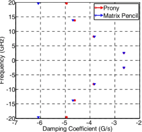
To compare the methods, we first consider a simple antenna such as a dipole. The length of the dipole is L = 50 mm and its diameter D = 0.67 mm, that is a ratio L/D equal to 75. There are four resonances between 0 and 22 GHz: at 2.67 GHz, 8.20 GHz, 13.75 GHz and 19.34 GHz. Using CST Microwave Studio, we simulate in time domain the farfield transient backscattered response of the dipole antenna illuminated by a short pulse. The backscattered transient response is given in Fig. 1.
Now we compare the TLS-Prony and the TLS-MP methods in presence of noise. A Gaussian white noise is added to the antenna response to obtain different Signal to Noise Ratio (SNR) from 0 to 80 dB.
First, Fig. 2 shows poles extracted from the non-noisy dipole antenna response with both methods. Fig. 3 presents the Mean Square Error (MSE) between the dipole response and the reconstructed response with poles and residues for the different values of SNR. Solid lines present the MSE when all extracted poles are used. Dashed lines present the MSE when only the physical poles are considered.
The MSE is almost the same with the two methods. For low SNR (0 – 10 dB), some mathematical poles are extracted by
both methods and, when used for the reconstruction, allow to find a very low MSE (lower than 0.4%). But they have no physical sense. For higher SNR, dashed line and solid line are merged. Now, for each method, we show the relative error between pole extracted from a non-noisy response and pole extracted from a noisy one. Fig 4 and Fig 5 present the relative error on the resonant frequency and on the damping coefficient of the first pole, respectively.
Fig. 1 Backscattered transient response of the dipole
Fig. 2 Poles extracted with the two methods
Fig. 3 MSE of the reconstructed response
Results with the two methods are very close. Resonant frequencies of the first pole are correctly extracted by the two methods (relative error lower than 1.7%). Damping
coefficients seem to be better extracted by the TLS-MP method especially for low SNR. These results are the average of fifteen samples of noisy data.
Fig. 4 Relative error on the frequency of the first pole
Fig. 5 Relative error on the damping coefficient of the first pole
A. Application to Ultra Wide Band (UWB) antenna
We now consider a UWB antenna developed by C. Marchais [8]. It is a wide slot stripline antenna fed by a fork-like tuning stub. This antenna is matched between 3 and 12 GHz (S11 under -10 dB).
Fig. 8 shows poles extracted from the non-noisy UWB antenna backscattered response with both methods. Eight pairs of poles are extracted with both methods and results are very close.
Same as the previous application, a Gaussian white noise is added to the UWB antenna backscattered response to obtain different SNR from 0 to 80 dB. Fig. 9 shows the MSE of the reconstructed response using poles and residues for different values of SNR.
The MSE is very low (lower than 0.06 %). Because of the high number of poles to extract (compared to the dipole case), it is much difficult to sort mathematical and physical poles. A sorting method is currently under active consideration but results are not presented here.
Now, for each method, we show the relative error between poles extracted from a non-noisy response and poles extracted from a noisy one. Fig 10 and Fig 11 present the relative error on the resonant frequency and on the damping coefficient of
0.5 1 1.5 2 2.5 3 -1 -0.5 0 0.5 1 Time (ns) N o rm al is ed amp lit ude Transient response -7 -6 -5 -4 -3 -2 -20 -15 -10 -5 0 5 10 15 20 Damping Coefficient (G/s) F requenc y ( G H z ) Prony Matrix Pencil 0 20 40 60 80 0 1 2 3 4 5 6 7 8 SNR (dB) MS E ( % ) Matrix Pencil
Matrix Pencil with physical poles Prony
Prony with physical poles
0 20 40 60 80 0 0.5 1 1.5 2 SNR (dB) R e la ti v e e rro r (% ) Matrix Pencil Prony 0 20 40 60 80 0 1 2 3 4 5 6 7 SNR (dB) R e la ti v e e rr o r (%) Matrix Pencil Prony
the pole whose the resonant frequency is 3 GHz, respectively. This pole is the only one always extracted by the two methods even for low SNR.
Fig. 8 Poles extracted with the two methods
Fig. 9 MSE of the reconstructed response
Fig. 10 Relative error on the frequency of the pole at 3 GHz
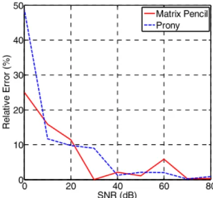
Once again, results of the two methods are close. Resonant frequencies are well extracted (relative error lower than 7%) but damping coefficients are better extracted by the TLS-MP method when SNR becomes low.
Fig. 11 Relative error on the damping coefficient of the pole at 3 GHz
IV. CONCLUSIONS
To our knowledge, these results are the first comparison of TLS-Prony and TLS-MP methods to analyze antenna transient backscattered responses. Although accuracies of the both methods are very close, the Matrix Pencil method seems to be slightly less sensitive to noise, especially for damping coefficients estimation. Complementary analyses are in progress to confirm these first interesting results, for example by using TLS-Prony and TLS-MP process through a shifting time window. The comparison will be also extended to poles and residues extracted in frequency domain, using the Cauchy ARMA process. The final objective of this work is to define a methodology, based on RCS measurement and SEM post processing, to obtain compact data able to analyse the main characteristics of an antenna.
ACKNOWLEDGMENT
This work was financially supported by the French Ministry for Defence (Direction Générale de l’Armement).
REFERENCES
[1] C. E. Baum, “On the Singularity Expansion Method for the Solution of Electromagnetic Interaction Problems”, EMP Interaction Note 8, Air Force Weapons Laboratory, Kirkland AFB, New Mexico, Dec. 1971. [2] S. Licul and W. A. Davis, “Unified Frequency and Time-Domain
antenna Modeling and Characterization”, IEEE Transactions on
Antenna and Propagation, vol. 53, No 9, pp. 2882–2888, Sep. 2005.
[3] C. Marchais, B. Uguen, A. Sharaiha, G. L. Ray and L. L. Coq, “Compact characterisation of ultra wideband antenna responses from frequency measurements“, Microwaves, Antennas & Propagation, IET vol. 5 , Issue: 6, pp. 671-675, 2011.
[4] R. Prony, “Essai expérimental et analytique sur les lois de la dilatabilité de fluides élastiques et sur celles de la force expansive de la vapeur d’alcool“, Journal école polytechnique, vol. 1, No 22, pp. 24-80, 1795. [5] Y. Hua and T. K. Sarkar, “Matrix Pencil Method for Estimating
Parameters of Exponentially Damped/Undamped Sinusoids in Noise”,
IEEE transactions on Acoustics, speech and signal processing, vol. 38,
No , pp. 814-824, May. 1990.
[6] T. K. Sarkar and O. Pereira, “Using the Matrix Pencil to Estimate the Parameters of a Sum of Complex Exponentials”, IEEE Antenna and
Propagation Magazine, vol. 37, No 1, pp. 48-55, Feb. 1995.
[7] MD. A. Rahman and KB. Yu, “Total Least Square Approach for Frequency Estimation Using Linear Prediction”, IEEE Transactions on
Acoustics, Speech and signal Recognition, vol. ASSP-35, No 10, pp.
1440-1454, Oct. 1987.
[8] C. Marchais, G. L. Ray and A. Sharaiha, “Stripline Slot Antenna for UWB Communications”, IEEE Antennas and Wireless Propagation
Letters, vol. 5, pp. 319-322, 2006. -15 -10 -5 0 -15 -10 -5 0 5 10 15 Damping Coefficient (G/s) F requenc y ( G H z ) Matrix Pencil Prony 0 20 40 60 80 0 0.01 0.02 0.03 0.04 0.05 0.06 SNR (dB) MS E ( % ) Matrix Pencil Prony 0 20 40 60 80 0 1 2 3 4 5 6 7 SNR (dB) R e la ti v e E rro r (% ) Matrix Pencil Prony 0 20 40 60 80 0 10 20 30 40 50 SNR (dB) R e la ti ve E rro r (% ) Matrix Pencil Prony