Application of analytical centrifugal-pump performance models in two-phase flow

CENTRIFUGAL-PUMP

PERFORMANCE MODELS IN

TWO-PHASE FLOW

by

JAMES EDWARD I/ORENCHAN S.B.M.E., Illinois Institute of Technology

(1982)

SUBMITTED TO THE DEPARTMENT OF MECHANICAL ENGINEERING IN PARTIAL FULFILLMENT OF THE

REQUIREMENTS FOR THE DEGREE OF MASTER OF SCIENCE

at the

MASSACHUSETTS INSTITUTE OF TECHNOLOGY August 1984

Copyright ( 1984 James E. Korenchan

The author hereby grants to MIT permission to reproduce and to distribute copies of this thesis document in whole or in part.

Signature of Author

Department of MECHANICAL ENGINEERING August 21, 1984

Certified by

David Gordon Wilson Thesis Supervisor

Warren M. Rohsenow, Chairman is

mT.

TECHu. 1partmental Committee on Graduate Studies

SsARCHIVES.

PERFORMANCE MODELS IN TWO-PHASE FLOW by

JAMES EDWARD KORENCHAN

Submitted to the Department of MECHANICAL ENGINEERING on August 21, 1984 in partial fulfillment of the requirements for the degree of MASTER OF SCIENCE.

Abstract

An analytical/semi-empirical model developed at MIT to correlate centrifugal-pump performance in two-phase flow was applied to experimental steam/water data produced by Combustion Engineering, Inc. on a 1/5-scale nuclear-reactor pump system. Performance parameters (head and flow coefficients, head-loss and head ratios, void fractions, and system pressures) were correlated and plotted for data in the first, second, and third flow quadrants. Results confirmed the dependence of two-phase pump performance on flow coefficient, void fraction, and system pressure. Experience was gained in the application of the MIT model to a new set of data.

The head-loss-ratio correlation was found to be effective for the first quadrant, but application in the second and third quadrants was not successful because of questionable formulation of the reverse-flow theoretical performance. Correlation by head-ratio was deemed to be more appropriate for the second and third quadrants.

Pump head degradation was found to decrease with increasing flow coefficient, and qualitative results generally agreed with those of other works. Correlation by system pressure and the distinction between upstream and pump-average parameters were stressed in this analysis.

Thesis Supervisor: Title:

David Gordon Wilson

ACKNOWLEDGEMENTS

I am deeply grateful to Professor David Gordon Wilson, whose expertise, advice, support, and personality enabled me to undertake and complete this research with professional exhilaration and fulfillment.

I affectionately appreciate the continued support of the members of my family, especially my parents, whose faith and love have been inspirational in all of my endeavors.

I am also grateful to my friends, both old and new, who have enriched my educational and social experience at MIT.

Finally, I wish to thank the General Motors Corporation, my employer, for sponsoring these graduate studies at MIT through the GM Fellowship Program.

TABLE OF CONTENTS

Page TITLE PAGE 1 ABSTRACT 2 ACKNOWLEDGEMENTS 3 TABLE OF CONTENTS 4 LIST OF FIGURES 6 LIST OF SYMBOLS 8 Chapter 1: INTRODUCTION 10 1.1. Background 10 1.2. Previous Work 11 1.3. Purpose 12

Chapter 2: MIT ANALYTICAL MODELS 13

2.1. Theoretical-Performance Derivations 13 2.2. Head-Loss-Ratio Method 18 2.2.1. General description 18 2.2.2. First-quadrant application 19 2.2.3. Second-quadrant application 21 2.2.4. Third-quadrant application 22

Chapter 3: APPLICATION TO C-E DATA 23

3.1. C-E Project Background 23

3.2. C-E Project Description 23

3.3. Correlation Parameters 25

3.5. Second-Quadrant Results 40

3.6. Third-Quadrant Results 44

Chapter 4: INTERPRETATION OF RESULTS 49

4.1. General Observations 49

4.2. Effect of System Pressure 51

4.3. Effect of Pump Inlet-to-Outlet Variations 52

4.4. Comparison with Other Works 52

Chapter 5: CONCLUSIONS AND RECOMMENDATIONS 54

5.1. Usefulness of C-E Data 54

5.2. Applicability of MIT Model 54

5.3. Recommendations for Model Use 54

APPENDIX A: C-E TEST PUMP DIMENSIONAL DATA 56

APPENDIX B: C-E STEADY-STATE FLOW DATA 60

B.1. First-Quadrant, Single-Phase Data 61

B.2. First-Quadrant, Two-Phase Data 64

B.3. Second-Quadrant, Single-Phase Data 69

B.4. Second-Quadrant, Two-Phase Data 70

B.5. Third-Quadrant, Single-Phase Data 71

B.6. Third-Quadrant, Two-Phase Data 72

APPENDIX C: CORRELATION DATA 73

C.1. First-Quadrant Data 73

C.2. Second-Quadrant Data 79

C.3. Third-Quadrant Data 80

Page FIGURE 2-1: VELOCITY TRIANGLES AT IMPELLER INLET AND OUTLET 14 FIGURE 3-1: COMBUSTION ENGINEERING TEST SECTION SCHEMATIC 24 FIGURE 3-2: HEAD COEFFICIENT i' VS. FLOW COEFFICIENT 4, 30

FIRST QUADRANT, SINGLE PHASE

FIGURE 3-3: HEAD COEFFICIENT iJ' VS. FLOW COEFFICIENT

4,

31 FIRST QUADRANT, SINGLE PHASE, 0.00 <

4

< 0.25

FIGURE 3-4: HEAD COEFFICIENT J)' VS. FLOW COEFFICIENT

4,

32 FIRST QUADRANT, TWO PHASE

FIGURE 3-5: HEAD COEFFICIENT 1' VS. FLOW COEFFICIENT

4,

33 FIRST QUADRANT, TWO PHASE, 0.00 <

4

< 0.25

FIGURE 3-6: HEAD-LOSS RATIO H* VS. AVERAGE VOID FRACTION cy 34 FIRST QUADRANT, CORRELATED BY FLOW COEFFICIEN ,

0.01 <

4

< 0.16

FIGURE 3-7: HEAD-LOSS RATIO H* VS. AVERAGE VOID FRACTION a 35 FIRST QUADRANT, CORRELATED BY FLOW COEFFICIENT ,

0.16 <

4

< 0.35

FIGURE 3-8: HEAD-LOSS RATIO H* VS. AVERAGE VOID FRACTION a 36 FIRST QUADRANT, CORRELATED BY FLOW COEFFICIENf

4),

0.30 <

4

< 0.45

FIGURE 3-9: HEAD-LOSS RATIO H* VS. AVERAGE VOID FRACTION a _tVg' 37 FIRST QUADRANT, CORRELATED BY SYSTEM PRESSURE p

FIGURE 3-10: HEAD-LOSS RATIO H* VS. UPSTREAM VOID FRACTION a _ups' 38 FIRST QUADRANT, CORRELATED BY SYSTEM PRESSURE p

FIGURE 3-11: HEAD RATIO " /4' VS. AVERAGE VOID FRACTION , 39 FIRST QUADRANT, CORRELATED BY SYSTEM PRESSUR 'p

FIGURE 3-12: HEAD COEFFICIENT J' VS. FLOW COEFFICIENT 4, 41 SECOND QUADRANT, SINGLE PHASE

FIGURE 3-13: HEAD COEFFICIENT *' VS. FLOW COEFFICIENT

4,

42 SECOND QUADRANT, TWO PHASE

FIGURE 3-14: HEAD RATIO

~t/sp'

VS. AVERAGE VOID FRACTION , 43 SECOND QUADRAN , CORRELATED BY FLOW COEFFICLNT 4

FIGURE 3-15: HEAD COEFFICIENT i4' VS. FLOW COEFFICIENT

f,

45 THIRD QUADRANT, SINGLE PHASE

FIGURE 3-16: HEAD COEFFICIENT *' VS. FLOW COEFFICIENT

4,

46 THIRD QUADRANT, TWO PHASE

FIGURE 3-17: HEAD-LOSS RATIO H* VS. AVERAGE VOID FRACTION 0 47

THIRD QUADRANT, CORRELATED BY FLOW COEFFICIEN

FIGURE 3-18: HEAD RATIO 't. /*'. VS. AVERAGE VOID FRACTION a , 48 THIRD QUADRANT, CORRELATED BY FLOW COEFFICIE T

Nomenclature

A flow area

Ct Pv

a two-phase property function

-b blade width 1- P

C absolute fluid velocity

d diameter

ftp two-phase flow function

g gravitational acceleration = 9.81 m/s 2 = 32.2 ft/s2

ge gravitational constant = 1.00 (kg m)/(N s2) = 32.2 (ibm ft)/(lbf s2)

H head

H head-loss ratio AHo°tpth

-

AHO'tP

h enthalpy AHo,sp,th AHo,sp

K geometric constant mh mass flow per unit time N pump impeller speed, rpm

Ns pump specific speed, (rpm)(gpm)0.5/(ft)0'7 5 p fluid pressure

Q volumetric flow per unit time

r radius

s slip-velocity ratio t impeller blade thickness u impeller peripheral velocity V fluid velocity

W fluid velocity relative to impeller W work done by impeller per unit time x _{flow quality -_ mv/mT}

z number of impeller blades

z elevation

ta _{area void fraction - AV/AT}

cx angle of fluid velocity C relative to meridional direction Sangle of fluid velocity W relative to tangential direction [3' impeller blade angle relative to tangential direction

A property or parameter change b flow deviation angle --

0'

- 1

11 impeller flow slip factor - C02/C02,th

p fluid density

flow coefficient - Cm/u i work coefficient - gcAho/u 22

ý'

Ihead coefficient -- gAH/U22 W pump impeller angular speed, rad/s

Subscripts

o

total, static plus dynamic, stagnation value

1

flow plane at (normal) entrance to impeller

lh

hub (inner) intersection of this plane

is

shroud (outer) intersection of this plane

2

flow plane at (normal) exit of impeller

2i

inner-shroud intersection of this plane

20 outer-shroud intersection of this plane

3

flow plane at (normal) entrance to diffuser

avg

arithmetic average

be

best-efficiency point, design point

L liquid

m meridional, normal to peripheral

m mean effective

rated rated conditions

sp single-phase

T total, liquid plus vapor

th theoretical

tp two-phase

ups upstream

V vapor

1. INTRODUCTION

1.1. Background

The United States nuclear industry employs centrifugal pumps in the primary coolant circuits of the majority of pressurized water reactors (PWRs). These pumps circulate light water under subcooled, pressurized conditions through the core and steam generators. One possible failure mode affecting the ability to cool the core is the loss-of-coolant accident (LOCA). A LOCA is envisioned as a full or partial rupture of the piping at any point in the closed-loop system. During the transient period immediately following a rupture, a blowdown process occurs which reduces the loop pressure (of the order of 14000 kPa or 2000 psi) to near atmospheric pressure. The duration of this depressurization transient depends on the extent of the rupture. Pressurized water flashes into steam through the loop, producing two-phase flow conditions. The performance of the pump(s) in two-phase flow is problematic and is the subject of current research.

The pressure difference between the coolant water and the atmosphere is many times larger than the normal operating pressure rise through the pump (of the order of 700 kPa or 100 psi). Therefore, water will flow toward the rupture regardless of its location relative to the pump, at least in the early part of the transient depressurization. If the pipe break were to occur near the discharge side of the pump, the resulting flow could be well above the pump operating range (i.e., forced flow). In general, any combination of forward (normal) flow through the pump and forward (normal) impeller rotation is known as first-quadrant operation. A break occurring on the suction leg of the pump would likely cause reverse flow through the pump. _{The conjunction of reverse pump flow and forward rotation is called} second-quadrant operation. Surmising further, the turbining action of reversed flow might reverse the impeller rotation, if there is no mechanical anti-reverse device; such a condition is called third-quadrant operation. Fourth-quadrant operation (forward flow and reversed

rotation) is inconceivable from a practical point of view.

The behavior of the centrifugal pump under two-phase flow conditions must be understood and predictable in order to justify a given course of action in the event of a LOCA. Consequently, research effort has been directed toward the modeling of the two-phase pump characteristics; the desired result is the application of reliable models in the nuclear industry.

1.2. Previous Work

Prior to 1977, there were several empirical models for two-phase pump behavior. Each model made use of some form of a head-degradation factor which related two-phase performance characteristics to single-phase characteristics at given flow conditions. These models differed primarily in the form of the factor and in the parameters used to correlate the empirical data. In general, the applicability of each model as a predictive tool was limited to the particular pump system and flow arrangement from which the experimental data were generated. A review of these models was conducted by Wilson, et al. [1977].

A semi-empirical method developed by J. Mikielewicz and D. G. Wilson at MIT (Wilson, et al. [1979]) defined a head-loss ratio as the ratio of the pump head losses in two-phase flow to the head losses in single-phase flow at the same flow coefficient. Subsequent testing on a low-pressure, air/water pump facility at MIT yielded acceptable model correlation. Head-loss ratio was found to be a function of void fraction and flow coefficient (flow regime, in general), and the model exhibited adequate predictive capabilities. Furthermore, the model provided analytical justification for applying the results of one pump system to other pump systems.

In response to a lack of a sufficient data base, the Electric Power Research Institute (EPRI) contracted Combustion Engineering, Inc. (C-E) of Windsor, Connecticut to generate a library of single- and two-phase pump performance data. The C-E test pump and its local

piping were constructed to a 1/5 geometric scale of the Palisades nuclear reactor system. Both steady-state and transient data were collected in flow conditions, temperatures, and pressures anticipated during a LOCA. The final report was published through EPRI (Kennedy, et al.

[19801).

1.3. Purpose

The intent of this current research was to apply the overall MIT analytical model to the C-E two-phase pump data and to examine the effectiveness of the model by data correlation and comparison with earlier results. Expected model weaknesses in the treatment of the variation of two-phase flow parameters through the pump and system pressure effects were given special attention.

The ultimate object of this investigation is to evaluate the MIT model through intensive application of data from an outside source (namely, Combustion Engineering). The discovered strengths and weaknesses of the model will help to define the limits of its applicability as a predictive tool.

2. MIT ANALYTICAL MODELS

The MIT semi-empirical analytical method focuses on the calculation of the head-loss ratio which relates experimental head characteristics with ideal single- and two-phase performance. This section describes the development of the ideal, theoretical performance relations and the application of the head-loss-ratio method in each of the first three quadrants. The presentation follows that given by Chan

(1977]

and Wilson, et al. [1979].

2.1. Theoretical-Performance Derivations

Along any given streamline through the pump, the Euler equation relates the change of enthalpy of, or work done by, the fluid to the change in angular momentum of the fluid into and out of the impeller.

W

- ch o gc(ho2- ho0 l)= 2C02 - ulC1 (2-1)

Equation (2-1) is of general validity for single- or two-phase flow assuming steady and adiabatic conditions.

The general one-dimensional, single-phase-flow velocity triangles for the impeller inlet and outlet are shown in Figure (2-1). The relative flow angle at impeller outlet,

02,

is equal to the blade angle, 12, less the angle of deviation, b, due to slip.

P2 = -2 Cm2 tan 2 = u2 - C02 C -C C02 - 1- Cm2 U2 _{u2tan 02}

U1

0·1

FIGURE 2-1: VELOCITY TRIANGLES AT IMPELLER INLET AND OUTLET Co2,th

axial-entry pumps with higher specific speeds.

C01

tan o -=

ml

C01 Cmltan aol Cm tan

1

U₁ U_{1 U}

1

Letting the flow coefficient,

4,

be defined as

Cm

and the work coefficient,

4,

be defined as

gcAh_o 2 U2

the Euler equation for a centrifugal pump in single-phase flow becomes

Cm2 Ul2 - UCml

m

t a n 1 Q•--u2tan 02 =-2 d S1 _{(L)2 (1 - tan} ) tan 02 d2

We choose to model two-phase flow as two separate mass flows, liquid and vapor, with presumably different values of velocity, C_O and Cm, at the impeller inlet and outlet. Euler's equation becomes

C

_(L2

C

_eV2 #tp=(1 2g "2

d

1)

H

(

d

2 - X) COL u1

By assuming that both the liquid and vapor streams leave the impeller in the same direction

(2-2)

U2 u C ovl₁ + x₁ --u1

(relative angle 32), we can derive from the velocity triangles, as before, u2tan 02 )2 + x2 utan 2) u a CmL1tan 1 - mV1 -

()2

₍₁

_-

_xI)

_-

_Cm

+

_{an )]}

_(2-3)

d

u

u

From continuity and the definition of void fraction, ax, we have at the outlet

CL2 T(1 - X2) mL2 PL2AL2 PL2(1 - 02)AT2 mlV2 IITX₂ mV2 Pv2Av2 PV2 %2AT2

and similarly for the impeller inlet. Here AT is the normal flow area at inlet or outlet. We can define a two-phase flow coefficient

lmT (•tp

=---T-PtpATu

where the two-phase density is related to void fraction the same as specific volume is related to flow quality

Ptp (1 - )PL + cxpv Substituting into equation (2-3), we obtain

ý)tp

=

1

_tan

1 +

--

2

(

1

-

x2

)

2

+

2

X2

2

)]

02

1

- ₂ t PL2 (t2 PV2

d ( 11 - ktp₁tan 1 PL

-+

a 1 P

x

2

(2-4)

Equation (2-4) can be simplified by defining a two-phase property function

PV

a

1-aP

L

and a slip velocity ratio between the two phases

Cv CL

By continuity and the above definitions, we can derive

as

x =

1+ as

Making these substitutions, the Euler equation for two-phase flow in a centrifugal pump becomes

ftp2tp2 dz

tp 1 - ()2 (1 - ftpldtpltan 1) (2-5) tan

02

_d2

where we have defined a two-phase flow function

(1I + a)(1 + as2)

tP

_{(1 + as)}

2

In a single-phase flow, we have a = a = 0 and, thus, ftp = 1.0 ; consequently, equation (2-5) becomes identical to the single-phase form, equation (2-2). In homogeneous two-phase flow, s = 1.0 (i.e., no slip), and again the two-phase flow function, ftp, is unity (yielding equation (2-2) for the theoretical two-phase head).

2.2. Head-Loss-Ratio Method

2.2.1. General description

The change in enthalpy through the pump is most effectively determined by measuring the change in total head across the pump. The total head is defined as

P₂ - pl V₂2 - V12

AH + + (zP - z2) (2-6)

S Pg/gc 2g

and represents the change in fluid energy by virtue of its pressure and elevation (static-head change) and its velocity (dynamic-head change). For adiabatic, inviscid flow it can be shown that the change in total head is directly proportional to the change in enthalpy through the pump; in fact, we find that gAHo = gcAho . We define a head coefficient as

gAH_o gcAho

' -- -= = 1)h (2-7)

U22 U22

and note that the head and work coefficients are identical under the stated conditions. The head-loss ratio, H*, is defined as

H

(2-8)

AH -zaH0 ,tp _ tp,th - (2-8)

o,sp,th -AHo,sp sp,th sp

which is the ratio of the two-phase head losses to the single-phase head losses at the same flow coefficient. _{The theoretical head coefficients are calculated from some form of the ideal} Euler equation (2-5).

The head-loss ratio, essentially a function of flow regime, is the key correlating parameter of the MIT performance model. The head losses which the ratio empirically relates are due to flow-separation, wall-friction, and the interaction of individual phases (two-phase

flow only). By normalizing two-phase head losses to single-phase losses, as opposed to normalizing the two-phase head to the single-phase head (,'(p/,'p), theoretical performance has been introduced along with empirical performance. In this way, it is anticipated that the two-phase performance dependence on a particular pump geometry is diminished.

Plots of head-loss ratio against void fraction for specified flow coefficient ranges form the semi-empirical basis for two-phase performance predictions. From the H* curves of one pump, the two-phase head coefficient of another pump can be calculated for a given void fraction and flow coefficient (provided the desired flow coefficient is in the range of the former pump's experimental range). The accuracy of this prediction can be properly judged only after a library of head-loss-ratio correlations are produced for pumps of varying specific speeds and geometries.

2.2.2. First-quadrant application

For a centrifugal pump operating in the first quadrant (forward flow, forward rotation), the angular momentum at the impeller inlet is very small compared with that at the outlet. If we assume that there is no inlet "swirl" or prerotation, then the Euler equation (2-1) becomes

gCAho = u C02

and the derived two-phase flow equation (2-5) simplifies to

ftp2 tp2

t 1p -1 _(2-9)

tan ₀₂

where the equivalence of the work and head coefficients has been assumed (adiabatic, inviscid flow; equation (2-7)).

The theoretical relation for first-quadrant operation can be further simplified by the fact that the two-phase flow function, ftp, is close to unity for practical (LOCA) conditions. Using

values of two-phase slip, s, based on a correlation by Thom [1964], ftp has been shown (Wilson, et al. [1977]; Chan [1977]) to be generally less than a value of 1.05 for steam-water flows with pressures greater than 500 psi (3400 kPa). Maximum values of ftp - 1.10 occur near high void fractions (•a=0.9). Consequently, we can choose to use

tp2

41p • 1 - (2-10)

tan P₂

as the theoretical two-phase Euler equation for a centrifugal pump operating in the first quadrant with no inlet swirl. This equation (2-10) is similarly valid for single-phase flow.

The remaining difficulty in using equation (2-10) is in knowing the slip factor, V, necessary to calculate the relative flow angle, 32. The slip factor is defined as

C,

C02

Ce2,th

and its relationship to the outlet flow angle can be obtained from Figure 2-1:

tan P2 1- (2-11)

1 - V + P02cot P'

Many methods of calculating V have been published. Stodola [1927] derived an appromixate relationship for the slip factor at the design operating point:

(x/z) sin

P2

Rbe = 1 - (2-12)

1 - 42,becot 02

Although it is unrealistic to assume that the slip factor and deviation angle remain constant over a large flow-coefficient range, the head-loss-ratio correlation will not be adversely affected to a great degree. Indeed, without adequate experimental measurement of the relative flow angle over an extended range of flow coefficients, there is no justification for other than a constant-deviation-angle assumption.

Wilson, et al. [19791 recommend the use of an empirical correlation by Noorbakhsh [1973] for determining the slip factor. This correlation produces a slip factor based on experiments made on five pumps of different geometries over somewhat extended flow-coefficient ranges. By obtaining results from a test pump of similar geometry, one attains some empirical justification in letting the slip factor vary over a given flow range.

2.2.3. Second-quadrant application

In the dissipative second quadrant (reverse flow, forward rotation) the two-phase Euler equation (2-5) cannot be applied directly because the flow angles at impeller inlet and outlet are not easily calculable. Also, the first-quadrant assumption of negligible prerotation is unrealistic for the second quadrant. Instead, Wilson, et al. [19791 use the geometry of the pump diffuser (inlet for reverse flow) and the impeller inlet (outlet for reverse flow) to derive the fluid angular momenta for use in the Euler equation (2-1). The critical assumptions are

- the relative outlet flow angle from the impeller in the second quadrant is equal to the relative inlet flow angle for the first quadrant, l,, measured from a plane through the axis and at the best-efficiency point; and

- the axial velocity, Cmi, is radially uniform.

The final result, which does not make a distinction for two-phase flow (i.e., ftp = 1.0) is

K( r1h )2 1 be Q Q tan _e₃

r'

= K( - 2)2 _r w _(2-13)

K

-

1 + -- + (

)

3 rls r₁s

and we note that the volumetric flow rate, Q, is negative in the second quadrant and that the angular speed, w, is positive.

2.2.4. Third-quadrant application

We make the same assumptions in the third quadrant (reverse flow, reverse rotation) that were made in the second. A similar derivation yields

Q tan a3 be Q ₍₂₁₄₎

ab' -- - K( - )2 1 _(2-14)

27b3r22w rls ) Qbe

where K is the same geometric factor as before and we note that both Q and w are negative in the third quadrant.

3. APPLICATION TO C-E DATA

3.1. C-E Project Background

The jointly-funded Combustion Engineering and Electric Power Research Institute project, entitled Pump Two-Phase Performance Program, came into existence as the result of a U. S. Atomic Energy Commision (AEC) request in 1973. The AEC sought programs for obtaining experimental information which would enable the development of more refined analytical modeling of pump performance under hypothetical LOCA conditions. The objective of the C-E/EPRI project was, therefore, to obtain sufficient steady-state and transient, single- and two-phase empirical data to substantiate present and ultimately improved mathematical models used for LOCA analysis. A full description of the project details and results appears in the C-E final report (Kennedy, et al. [1980]).

3.2. C-E Project Description

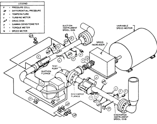
As stated earlier, the C-E project used a 1/5-scale model of the Palisades Nuclear Power Plant reactor coolant pumps (see Appendix A for pertinent dimensions and rated performance conditions). In addition, the suction and discharge piping adjacent to the pumps was modeled to the same scale; however, the pump axis was positioned horizontally instead of vertically as in the reactor system. In steady-state testing, steam from a pressure boiler would be mixed with pressurized water at saturated conditions and directed through the test pump in either the forward or reverse direction, depending on the arrangement of the reversible piping. Transient tests to simulate the pressure degradation and two-phase phenomena of a blowdown following a rupture were made by establishing specified steady-state conditions and utilizing a rupture diaphragm.

The basic elements of the test system with the locations and types of accompanying instrumentation are shown in Figure 3-1. _{The instrumentation included temperature sensors,}

pressure tranducers, gamma densitometers, drag discs, turbine meters, and flow orifices. Parameters either directly measured or derived from other measurements include pump suction and discharge pressures, temperatures, densities, velocities, volumetric flow rates, and void fractions. In addition, pump speed, shaft torque, and the mass flow rate of the individual steam and water flows entering the system were recorded. Data acquisition systems scanned the instrumentaion, recording time-averaged results and measurement drift.

Most of the test program was devoted to forward pump flow and forward impeller rotation (first quadrant). Much less emphasis was placed on the reverse-flow quadrants because reactor pumps are fitted with anti-reverse-rotation devices and a reverse flow transient would not last long before the pump impeller slowed to a halt. Fourth-quadrant combinations of forward flow and reverse rotation were omitted from the program. For each quadrant of operation tested, a comparable number of single-phase steady-state test runs and two-phase test runs were performed.

3.3. Correlation Parameters

In single-phase pump flow, the performance is correlated by parameters which are derived from the basic measurements of volumetric flow rate, pump head, pump speed, and fluid density. For two-phase flow, void fraction and system pressure are also necessary to define the performance. The head-loss-ratio correlation method requires the calculation of two key parameters: the flow coefficient and the head coefficient. The flow coefficient used here will be defined with respect to the impeller exit, regardless of the flow quadrant involved. Consequently, we have (dropping the subscript 2 on 4)

C ₂

U2

Q

C --` Cm2 A2 and S2 r2,mN 60

The net flow area at impeller exit, A2, is calculated in Appendix A . The head coefficient,

4'

is calculated using equation (2-7) where the total head, AHo, is given by equation (2-6). Several decisions were made in the present analysis with regards to the selection of the particular measurements used to calculate the correlating parameters; the completeness of the C-E test program afforded various choices. First of all, the static-pressure rise across the pump was taken from suction flange to discharge flange. The C-E data also offered a leg-to-leg Ap; pressure cells were located within the main instrumentation sections several feet ahead of and behind the test pump. Combustion Engineering's own data presentations utilized this leg-to-leg pressure rise (which included the losses in two suction pipe elbows, Figure 3-1) because of the sensor proximity to the other instrumentation (turbine meter, densitometer, etc.) and because of their desire to model the pump system, including adjacent piping. The decision here to use the flange-to-flange Ap was made because the analytical model incorporates only the pump (specifically, the impeller) and not any piping losses.

During two-phase flow conditions, significant variations in parameters occur from pump suction to pump discharge; the change in absolute pressure affects the thermodynamic equilibrium between the phases. The variations are most pronounced at low-to-medium void fractions, 0.0 < a < 0.5 . _{In this analysis, the volumetric flow rates, two-phase densities,}

and void fractions used were arithmetic averages of the suction and discharge measurements. One reason for this choice is that the fluid averages are more representative of the intra-impeller flow conditions. Also, the use of either the upstream or downstream measurements alone would be less accurate than the use of the averages because of the distance of the

sensors from the test pump. The effect of the parameter variations on the application results is analyzed in Chapter 4.

The void fractions and fluid densities used in this analysis were those computed by Combustion Engineering through the application of an energy balance. Measured mass flow rates of the individual steam and water flows were used to determine the quality and hence the density at mixing based on known saturation densities. Energy corrections for heat gains and losses in the piping legs and for the pump work were made based on temperature, pressure, and flow measurements through the test section. Void-fraction readings (from which density could be calculated) were also obtained through the use of three-beam gamma densitometers, but interpretations of these readings are irresolute because of the non-uniform phase distributions that usually existed in the piping. Furuya [1984] examined the C-E densitometer data and noted that the steam and water flows separated noticeably as they traversed the two 900 elbows ahead of the pump inlet. The variations in the densitometer readings, sometimes as much as 5:1 between beams, preclude their meaningful use.

Calculation of void fraction by the energy balance described above ignores the phenomenon of slip (different relative velocities of steam and water). In fact, the energy-balance void fraction is the volumetric quality of the flow; it is not the actual void fraction, based on cross-sectional area, which would be properly measured by a gamma densitometer. By using the volumetric quality to represent the void fraction, we are assuming that the flow is homogeneous, that is, s = 1.0 . This assumption does not diminish the value of volumetric quality as a correlating parameter, however. Indeed, Manzano [1980] concluded that the flowing void fraction (volumetric quality) was a better correlating parameter than the actual void fraction, based on results from a low-pressure, air/water test rig at MIT. One justification for the use of the volumetric quality is that the pump impeller blades tend to cut across any non-uniform phase distributions at the pump inlet, creating a more homogeneous mixture.

Since two-phase flows occur at saturated conditions, the system pressure is an indication of the thermodynamic state of the fluid. The average absolute pressure of the fluid within the pump section was included in this analysis as a correlating parameter. The effect of system pressure on two-phase pump performance is analyzed in Chapter 4.

3.4. First-Quadrant Results

The C-E steady-state, first-quadrant flow data appear in Appendix B along with flow and head coefficients for each test point. The least-squares, fourth-degree polynomial fit of the single-phase data (including both water and steam points) was found to be

= 0.4692 - 0.053954 - 8.334ý2 + 14.1043 - 35.84ý4 sp

for the flow coefficient range

0.00 <

4

< 0.45

The root-mean-square error in

(s

was 0.0406 for all test points and was 0.0170 for those test points with • > 0 . The single-phase points and curve fit appear in Figures 3-2 and 3-3. Several (13%) of the single-phase points listed in Appendix B were omitted from the curve-fitting process because they deviated significantly from the rest. Most of these anomalies occurred at high flow coefficients (k > 0.25).

Calculation of the slip factor, R, at the design operating point by the Stodola equation (2-12) yielded vi = 0.57 , while use of the empirical correlation by Noorbakhsh resulted in a roughly constant

p~

F- 0.58 over the flow coefficient range 0.07 <

4

< 0.22 . Combining equations (2-10) and (2-11) gives

~ttp,th - ý)sp,th = I 1 -

ta

and substitution of ftanctor givesthe Noorbakhsh slip

and substitution of the Noorbakhsh slip factor gives

which was the theoretical relation used for computing the head-loss ratio H*.

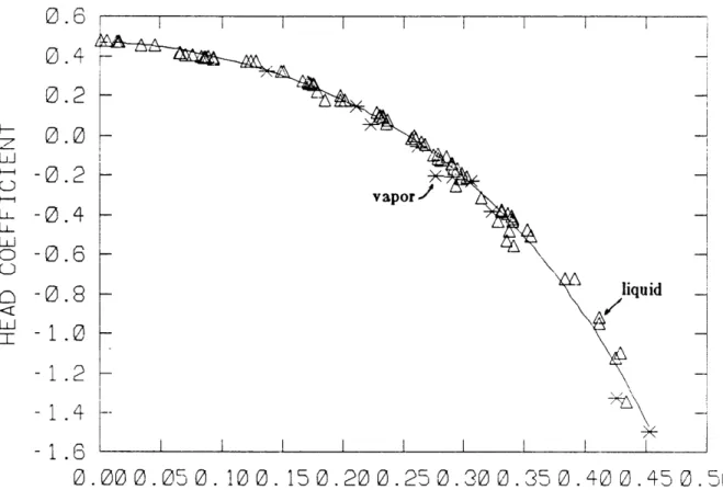
The system operating pressure most prevalent in the C-E steady-state, two-phase data was 1000 psi (6900 kPa). Consequently, when pressure is not the main correlating parameter, first-quadrant plots contain only test points with pressures near 1000 psi. Plots of the two-phase test points, correlated by void fraction and illustrating their relation to the single-two-phase and theoretical curves, are given in Figures 3-4 and 3-5.

The head-loss ratios, H*, and head ratios,

,tjp/

bp

, for the two-phase test points are given in Appendix C . Listed with each point for correlation purposes are the upstream and average void fractions and the system pressure.

Plots of head-loss ratio and head ratio against void fraction, correlated by either flow coefficient or system pressure, are given in Figures 3-6, 3-7, 3-8, 3-9, 3-10, and 3-11. The curves sketched through the points are understood to be approximate correlating curves.

V0.O

0.4

0.2

0.0

-0.2

-0.4

-0.6

-0.8

-1.0

1.2

1.4

1.6

vapor I I I I I I I I

0. 00@0.050 . 100.150.200.250 .300.35 0.400

.450.50

FLOU COEFFICIENT

FIGURE 3-2: HEAD COEFFICIENT i' VS. FLOW COEFFICIENT 4, FIRST QUADRANT, SINGLE PHASE

? Ir_-

-0.

4

0.40

0.35

0

.

30

0.25

0.20

0.

15

0. 10

0

.

05

0

. 00

vapor

liquid

liquid 3

0.00

0.05

0.10

0.

15

0.20

FLOU COEFFICIENT

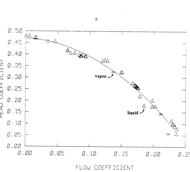
FIGURE 3-3: HEAD COEFFICIENT '' VS. FLOW COEFFICIENT 4,

FIRST QUADRANT, SINGLE PHASE, 0.00 < ý < 0.25

0.25

1

i .V_)

0.5

0.0

-0.5

-1.0

-1.5

-0.00 0.05 0.10 0.15

0.20

0.25 0.30 0.35

0.40 0.45

FLOJ COEFFICIENT

0.0 < at_avg 0.1 < ac 0.2 < otavg_avg 0.3 < av 0.5 < avg 0.7 < avg avg 0.9 < av avg 0.1 0.2 0.3 0.5 0.7 0.9 1.0

FIGURE 3-4:. HEAD COEFFICIENT

4'

VS. FLOW FIRST QUADRANT, TWO PHASE

COEFFICIENT C,

I c;~

0.5

z

0.4

LL 0

o

0.2

U

_0.1

0I

0.0

0 . i

0.00

0.05

0.

10

0. 15

0.20

0 . 25

FLOU COEFFICIENT

-X- 0.0 < at < 0.1 avg + 0.1 < c < 0.2 avg [] 0.2 < ag < 0.3_avg A 0.3 < oa < 0.5 avg 0 0.5 < o < 0.7 avg o 0.7 < at < 0.9 avg z 0.9 < a < 1.0 avg 950 < p < 1050 psi

FIGURE 3-5: HEAD COEFFICIENT 4' VS. FLOW COEFFICIENT 4, FIRST QUADRANT, TWO PHASE, 0.00 < ý < 0.25

A

4.0

3.5

3.0

2.5

2.0

1.5

1.0

0.5

p 0

0.0 0.1 0.2

0.3 0.4 0.5

0.6

0.7

0.8

0.9 1.0

AVERAGE VOID

FRACTION

ED 0.01 <

4

< 0.06

A 0.06 <

4

< 0.10

o 0.10 <

4

< 0.14 0 0.14 <

4

< 0.16 950 < p < 1050 psi

FIGURE 3-6: HEAD-LOSS RATIO H* VS. AVERAGE VOID FRACTION Na

FIRST QUADRANT, CORRELATED BY FLOW COEFFICIENT

4,

0.01 <

4

< 0.16

2.5 m

~

00 0

0

G

7F]

--AD K)~~

0.0 0.

1 0.2 0.3

0.4-

0.5 0.6 0.7 0.8 0.9 1.0

AVERAGE VOID FRACTION

D

0.16 < 4 < 0.20 A 0.20 < 4 < 0.24 O 0.26 < 4 < 0.30 0 0.30 < 4 < 0.35 950 < p < 1050 psi

FIGURE 3-7: HEAD-LOSS RATIO H* VS. AVERAGE VOID FRACTION o

FIRST QUADRANT, CORRELATED BY FLOW COEFFICIENf M,

0.16 < 4 < 0.35

2.0

o

H--1.5

0

_J

1.0

7-L

0.5

0 0 I 1 1 I 1 I I 1 I

I i I I I I I

0.0 0.1 0.2 0.3 0.4-

0.5

0.6 0.7

0.8

0.9

1.0

AVERAGE VOID

FRACTION

D

0.30 <

4

< 0.35

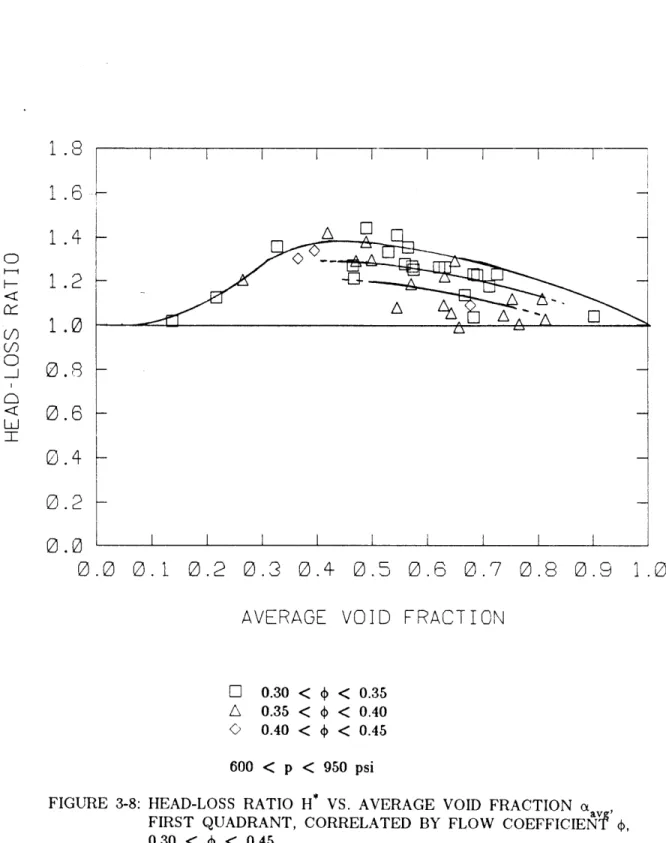
A 0.35 < 4 < 0.40 O 0.40 < 4 < 0.45 600 < p < 950 psi

FIGURE 3-8: HEAD-LOSS RATIO H* VS. AVERAGE VOID FRACTION a FIRST QUADRANT, CORRELATED BY FLOW COEFFICIENT , 0.30 <

4

< 0.45

1.8

1.6

1.4

1.2

1.0

0.8

0.6

0.4

0.2

0.0

SI I I I

0.0

0.1

0.2

0.3 0.4

0.5

0.6 0.7 0.8

0.9

1.0

AVERAGE VOID

0

470 < p < 490 A 840 < p O 950 < p

0 1110 < p

FRACTION

psi < 860 psi < 1030 psi < 1230 psi 0.134 <

4

< 0.162

FIGURE 3-9: HEAD-LOSS RATIO H* VS. AVERAGE VOID FRACTION a_av'E

FIRST QUADRANT, CORRELATED BY SYSTEM PRESSURE p

3.0

2.5

2.0

1.5

1.0

0.0

,_5.D

3.0

2.5

2.0

1.5

1.0

0.5

0.0 0.1

0.2 0.3

0.4

0.5 0.6 0.7 0.8 0.9

1.0

UPSTREAM

O 470 < p A 840 < p O 950 < p 0 1110 < p

VOID FRACTION

< 490 psi < 860 psi < 1030 psi < 1230 psi 0.134 <

k

< 0.162

FIGURE 3-10: HEAD-LOSS RATIO H* VS. UPSTREAM VOID FRACTION a(

FIRST QUADRANT, CORRELATED pBY SYSTEM PRESSURE FIRST QUADRANT, CORRELATED BY SYSTEM PRESSURE p

I A

1.2

1.0

0

S0.8

<

0.6

LiJ_-r

w

0.4

0.2

0.0

0.0

_{0.1 0.2 0.3}

_0.4-

_{0.5 0.6 0.7}

_0.8

_0.9

_1.0

AVERAGE VOID FRACTION

O 470 < p < 490 psi A 840 < p < 860 psi O 950 < p < 1030 psi O 1110 < p < 1230 psi

0.134 <

4

< 0.162

FIGURE 3-11: HEAD RATIO "j /*' VS. AVERAGE VOID FRACTION a FIRST QUADRANT, CORRELATED BY SYSTEM PRESSUR p

3.5. Second-Quadrant Results

The C-E steady-state, second-quadrant flow data appear in Appendix B, and the correlating parameters for two-phase performance are listed in Appendix C . The least-squares polynomial fit used for single-phase performance was

#b'p = 0.5301 + 1.0834 + 24.6742 + 5.04943 + 1.405ý4

for the flow coefficient range

-0.75 <

4

< 0.00

with a root-mean-square error in

bsp

of 0.0745 . The single-phase plot appears in Figure 3-12.

Theoretical performance for the second quadrant was calculated using equation (2-13). The theoretical-performance line is given in Figure 3-13 along with the second-quadrant, two-phase points and their relation to the single-two-phase curve.

Because the theoretical-performance line intersects the single-phase curve for the second quadrant, the head-loss ratio correlation is inappropriate. This observation is interpreted in Chapter 4. _{A plot of head ratio against void fraction for the second quadrant is given in} Figure 3-14.

I 7 i.,

10

t-S8

O LL

6

0 LLI

<:

4

2

(71

-0.8

-0.7

-0.6

-0.5 -0.4

-0.3 -0.2 -0.1

0.0

FLOU COEFFICIENT

FIGURE 3-12: HEAD COEFFICIENT 4' VS. FLOW COEFFICIENT

I,

z

LL 0 L( 0

<4

Li

w

2

-0.7

-0.6

-0.5

-0.4

-0.3

-0.2

-0.1

0.0

FLOU COEFFICIENT

-x

0.0 < a _avg < 0.1 + 0.1 <t a _avg < 0.2 0 0.2 < a < 0.3 A 0.3 < ag < 0.5_avg 0 0.5 < a _avg < 0.7 0 0.7 < a < 0.9 avg z 0.9 < ta < 1.0 avg 820 < p < 1160 psi

FIGURE 3-13: HEAD COEFFICIENT i' VS. FLOW COEFFICIENT

4,

SECOND QUADRANT, TWO PHASE

I iI I i ii i 0 0 4- Li

3.5

3.0

2.5

2.0

1.5

1.0

0.5

0.0

I I I I I

0.0 0.

1

0.2 0.3

0.A4

0.5

AVERAGE VOID

0.6 0.17 0.8 10.9

FRACTION

E

A C) 0 -0.67 <

4

< -0.36 -0.24 <

4

< -0.17 -0.16 <

4

< -0.08 -0.06 <

4

< -0.01 820 < p < 1160 psi

FIGURE 3-14: HEAD RATIO *' / ,' VS. AVERAGE VOID FRACTION ct

SECOND QUAD ANT, CORRELATED BY FLOW COEFFICIENT 4 0

1.0

i

4

3.8. Third-Quadrant Results

The C-E steady-state, third-quadrant flow data appear in Appendix B, and the correlating parameters for two-phase performance appear in Appendix C . The least-squares polynomial fit used for single-phase performance was

Vs = 0.2760 - 3.4124 + 28.3042 - 41.8843 + 97.454A for the flow coefficient range

0.06 < 4 < 0.30

with a root-mean-square error in I)' of 0.0131 . The single-phase plot appears in Figure 3-15.

Theoretical performance was calculated using equation (2-14). A plot of the two-phase points and their relation to the theoretical and single-phase performance curves is given in Figure 3-16. Plots of head-loss ratio and head ratio against void fraction for the third quadrant are given in Figures 3-17 and 3-18, respectively.

1.4

1.2

1.0

0.8

0.6

0.4

0.2

o- r• 0 .

0.05

0.

10

0.15

0.20

0

.25

FLOW COEFFICIENT

FIGURE 3-15: HEAD COEFFICIENT ý{' VS. FLOW COEFFICIENT 4, THIRD QUADRANT, SINGLE PHASE

0.30

I i I _ I

0.7

0.6

z

o 0.4

O 0

a

0.3

I

0.2

0.1

0.06 0.08 0.10 0.12 0.14 0.16 0.18 0.20 0.22 0.24

FLOU COEFFICIENT

-- 0.0 < av < 0.1 avg + 0.1 < co < 0.2 avg

A

0.2 < c < 0.3 avg A 0.3 < _avgv < 0.5 0 0.7 < ot < 0.7 avg O 0.7 < a < 0.9 avg . 0.9 < av _avg < 1.0 520 < p < 1010 psi

FIGURE 3-16: HEAD COEFFICIENT J' VS. FLOW COEFFICIENT 4, THIRD QUADRANT, TWO PHASE

1.6

1.4

1.2 -_

Ao

of

0.8 -

o

0

00.6

I

0.4

0.2

-0

.0

I

I

I

l

I

Ii

0.0 0.1 0.2 0.3 0.4 0.5 0.6 0.7 0.8 0.9 1.0

AVERAGE VOID FRACTION

]

0.08 <

4

< 0.12

A 0.15 <

4

< 0.16

O

0.19 <

4

<

0.24

520 < p < 1010 psi

FIGURE 3-17: HEAD-LOSS RATIO H* VS. AVERAGE VOID FRACTION a

i.6

I

1.4

1.2

]

0 E

A

:

1.0

m 0.8

0.6

0.4

0.2

-0.0 0.1 0.2 0.3 0.4 0.5 0.6 0.7 0.8 0.9 1.0

AVERAGE VOID FRACTION

O 0.08 <

4

< 0.12 A 0.15 <

4

< 0.16 0 0.19 <

4,

< 0.24 520 < p < 1010 psi

FIGURE 3-18: HEAD RATIO ' /ft's VS. AVERAGE VOID FRACTION ot

4. INTERPRETATION OF RESULTS

4.1. General Observations

The nature of the head-loss ratio is best illustrated by the two-phase plots of head coefficient against flow coefficient where the theoretical and single-phase performance curves have been included (Figures 3-4, 3-5, 3-13, and 3-16). The theoretical performance provides a geometrically-related reference from which to normalize the two-phase flow characteristics. The magnitude of the head-loss ratio is affected by the "distance" from the single-phase curve to the theoretical curve at a given flow coefficient as well as by the distance from the two-phase point. Since the difference between isp and 'th is greatest at higher

flow-coefficient magnitudes (for all three quadrants), we can expect H* to be closer to unity at high

4

regardless of any material changes in the two-phase flow physics. Simi!arly, we can expect the head-loss ratio to be largest for two-phase points at flow coefficients where the theoretical and single-phase characteristics are close in value (at low and design-point flow coefficients). Therefore, although the two-phase physics at different flow regimes does affect the head-loss ratio magnitude, a significant effect is "artificially" created by the theoretical performance formulation (specifically, from the constant-slip-factor assumption).

The magnitude of the head ratio, I'tp/iJ)p , for a given two-phase point is determined by the single-phase head-coefficient value in addition to the actual two-phase flow degradation. A problem in correlating by head ratio in the first quadrant is that the head ratio will become very large or negative at flow coefficients near where the head coefficient becomes zero. The head-loss ratio, however, avoids any problem in this region because of its definition and the fact that the theoretical line will never cross the single-phase curve.

In the second-quadrant results, the theoretical performance line intersected the single-phase performance curve (see Figure 3-13), causing large and negative head-loss ratios (Appendix C). Even if the theoretical line had only come close to the single-phase curve, the

head-loss-ratio correlation would have been adversely affected.

Obviously, the theoretical

relation used was not appropriate.

The polynomial fit of the single-phase data was strongly

quadratic, emphasizing that the second quadrant is almost entirely a dissipative region.

In

the formulation of the second-quadrant theoretical equation (2-13), the pump was treated as a

performance machine; evidently, such a model does not adequately represent the true,

dissipative second-quadrant performance.

(Under the constant-inlet-flow-angle or straight-line

assumption, though, the model was close to the actual characteristics).

Two-phase correlation

by the ratio of head losses is questionable in a quadrant where the performance is

characterized only by losses.

The head-loss ratio correlated the first-quadrant two-phase data well.

There was a

significant amount of data with which meaningful curves were generated, although more data

would be required to better complete the desired correlation ranges.

The effects of system

pressure and parameter variations from pump inlet to outlet for the first quadrant and the

comparison of the results with other works are discussed in the next sections.

Insufficient two-phase data were available in the second and third quadrants to

determine whether a correlation model, empirical or semi-empirical, is necessary at all.

Indeed, the third-quadrant two-phase points all fell close to the single-phase performance

curve, causing both the head-loss ratio and the head ratio to be near unity.

This fact

supports the accuracy of the measurement of two-phase density and the calculation of total

head used in this analysis.

Because of the uncertainty involved in the formulation of the

theoretical performance, head ratio would be a better correlation parameter for the second

and third quadrants.

The C-E data do exhibit a considerable amount of scatter.

Often the reasons are

because of the physical nature of two-phase flow:

unsteady flow oscillations, non-uniform

phase distributions, and irregular transitions of flow regime. Uncertainties in measurements

full investigation of the C-E data scatter, anomalies, and uncertainties was conducted by Kennedy, et al. [1980]. Dominant trends in head degradation related to void fraction, flow rate, and pressure were quite apparent despite data scatter. Subtle effects in two-phase pump performance (impeller speed and bubble-scale effects, for instance) would be difficult to discern from the C-E data.

4.2. Effect of System Pressure

The head-loss-ratio plot against void fraction for flows near the first-quadrant best-efficiency point (ýbe = 0.150) correlated by system pressure, Figure 3-9, clearly illustrates the effect of the system pressure on two-phase pump performance. The two-phase head-degradation effects are enhanced at lower pressures because there is a greater difference between the respective liquid and vapor densities at lower saturation pressures. The density difference amplifies such two-phase mechanisms as fluid centrifugal forces and bubble drag forces. Contrarily, higher pressures suppress the head-degradation effects. Judging from Figure 3-9, head-loss-ratio magnitudes can be expected to decrease gradually for system pressures greater than 1250 psi (8600 kPa) and to increase in some way for pressures less than 450 psi (3100 kPa).

System pressure must be included as a parameter in any head-degradation correlation of steam/water two-phase flow. However, system pressure is probably not as important for the correlation of non-condensible gas/water flows (so long as cavitation is avoided). For such flows, the pressure does not affect the gas/liquid density ratio in the same manner as for steam/water flows. Also, without condensation of vapor, density and void fraction will not vary significantly through the pump. _{The effect of these variations on the C-E} head-degradation correlations is discussed below.

4.3. Effect of Pump Inlet-to-Outlet Variations

The pressure variations in the two-phase flow traversing the pump cause constant adjustments of the thermodynamic equilibrium between the liquid water and steam. Two-phase density, volumetric flow rate, and void fraction vary from pump inlet to outlet. As explained in Chapter 3, the effects of density and flow rate variations were moderated by utilizing pump average values in the analysis. However, Figure 3-10 shows the result of correlating H* to the upstream void fraction for first-quadrant flows near the best-efficiency point. By comparison with the plot against average void fraction, Figure 3-9, we observe that the shape of the head-loss-ratio curve differs most in the low void fraction region, 0.0 < •t < 0.3 . Vapor condensation accounts for the marked difference in this region. Void fractions of as much as 10% at pump inlet can completely vanish by pump outlet due to condensation prompted by large pressure changes (small head degradation). At higher void fractions, the pump head is so degraded that void fraction does not vary as much, and the correlation curve shapes are similar.

The difference between the correlations by upstream and average void fraction, at least at the flow-coefficient range shown, is significant enough that it should not be neglected when using the correlations for predictive purposes. _{When only upstream data are available,} predictions could be made through utilizing some empirical correction of upstream void fraction and then entering the correlation curves plotted against average void fraction. Such an empirical correction, if workable, would eliminate the need for two sets of correlation curves.

4.4. Comparison with Other Works

The general shape of the head-loss-ratio curves for the first quadrant (Figures 3-6 through 3-10) agree well with curves generated by other MIT authors (Chan [1977], Manzano

[1980], Paik [1982], and Paran [1983]), and the physical reasons for the qualitative shape have been discussed elsewhere. However, the magnitudes of the head-loss ratios for similar flow-coefficient ranges do not agree well. Two reasons for these quantitative discrepancies are that different flow media were used (air/water (Manzano, Paran) or freon (Paik)) and that the overall pump efficiencies for each test system differed. Quantitative differences also exist for the head-ratio correlation. Because of these discrepancies, confidence in the application of the C-E data to pump systems that are not similar is diminished.

The magnitudes of H* were greatest at the lowest flow coefficients and decreased with increasing flow coefficient up to and beyond the best-efficiency flow, 4

be. Manzano's results agreed with this trend, but some applications by Wilson, et al. [1979] showed that the largest head-loss ratios occurred near ýbe. Certainly the smallest single-phase losses occur at the design point, but apparently there can be significant increases in the two-phase losses at low flow coefficients. The trend of decreasing head degradation with increasing flow coefficient was also noted on a 1/20-scale model pump tested by Creare/EPRI. Here, Patel and Rundstadler [1978] observed the formation of larger voids within the pump during low-flow-coefficient operation. The existence and effect of these larger voids for a given pump most likely depends on its specific speed and geometric scale.

The effects of vapor-bubble scale relative to the pump geometric scale have been analyzed or noted by Rundstadler and Dolan [1978], Murakami and Minemura [1978], and Furuya [1984], among others. The extent of the dependence of the head degradation on scale needs to be determined in order for the C-E results to be considered valid for the full-scale

5. CONCLUSIONS AND RECOMMENDATIONS

5.1. Usefulness of C-E Data

As a data base for evaluating improved head-degradation models of two-phase pump flow, the C-E data contained too much scatter, uncertainty, and system dependence. Only rough trends can be observed and correlated; subtle effects that a new model might attempt to incorporate would be obfuscated. For the evaluation of the semi-empirical MIT model, the C-E data trends have provided added insight. The most positive aspect of the C-E test program is that the test system was a scale model of a currently-employed reactor coolant pump and tests were run near actual system conditions. Therefore, for LOCA predictive purposes, the C-E data yield the most justifiable correlations at present. Application to other pumps of similar size and specific speed should also be effective.

5.2. Applicability of MIT Model

This research has confirmed the head-loss-ratio method as an acceptable means of correlating pump head degradation in two-phase flow, subject to the recommendations listed below. There are, however, still too many factors which render the correlation pump-specific. These factors include pump efficiency, geometric scale, inlet-piping configuration, and pump specific speed (centrifugal, mixed-flow, etc.). The MIT semi-empirical model was developed as an attempt to understand and to distinguish some of the two-phase pump-flow phenomena, but there yet exists a preponderance of empiricism in its application.

5.3. Recommendations for Model Use

As a result of this application of the MIT semi-empirical model to the C-E data, the following recommendations for use of the model are made.

- Unless an analytical formulation of slip factor, p, is developed which can confidently be applied to different pumps, a constant slip factor based on the design point, Itbe, should be utilized. Otherwise, the H* correlation results become

less reliable for predictive purposes.

- Head-loss ratio is an acceptable correlation method for the first quadrant, but its use in the second and third quadrants is disputable. For these latter quadrants, the primary difficulty is formulating an acceptable theoretical-head-coefficient relation. The purely empirical correlating factor 'jp/*'p can be used with greater success in the second and third quadrants.

- System pressure must be included as a primary correlation parameter along with flow coefficient, at least for cases where the flow contains a condensible vapor.

- For the purpose of predicting two-phase pump performance involving a condensible vapor, a distinction should be made between upstream and average void fraction for best results.