HAL Id: hal-01221716
https://hal.archives-ouvertes.fr/hal-01221716
Submitted on 16 Apr 2021
HAL is a multi-disciplinary open access archive for the deposit and dissemination of sci-entific research documents, whether they are pub-lished or not. The documents may come from teaching and research institutions in France or abroad, or from public or private research centers.
L’archive ouverte pluridisciplinaire HAL, est destinée au dépôt et à la diffusion de documents scientifiques de niveau recherche, publiés ou non, émanant des établissements d’enseignement et de recherche français ou étrangers, des laboratoires publics ou privés.
A new bond slip model for reinforced concrete
structures: Validation by modelling a reinforced
concrete tie
Chetra Mang, Ludovic Jason, Luc Davenne
To cite this version:
Chetra Mang, Ludovic Jason, Luc Davenne. A new bond slip model for reinforced concrete structures: Validation by modelling a reinforced concrete tie. Engineering Computations, Emerald, 2015, 32 (7), pp.1934-1958. �10.1108/EC-11-2014-0234�. �hal-01221716�
1
A new bond slip model for reinforced concrete structures.
Validation by modelling a reinforced concrete tie
C. Mang
CEA, DEN, DANS, DM2S, SEMT, LM2S , F-91191 Gif sur Yvette, France Also at : LEME, Université Paris Ouest, F-92410 Ville d’Avray, France L. Jason
CEA, DEN, DANS, DM2S, SEMT, LM2S , F-91191 Gif sur Yvette, France
Also at : IMSIA, UMR 9219 CNRS-EDF-CEA-ENSTA, Paris Saclay University, 91762 Palaiseau Cedex, France L. Davenne
LEME, Université Paris Ouest, F-92410 Ville d’Avray, France Corresponding author: L. Jason
ludovic.jason@cea.fr
Acknowledgments:
The first author would like to deeply thank T. Charras and S. Pascal for their helpful discussions in the elaboration and the implementation of the interface element in the finite element code Cast3M. The authors also thank AREVA for their helpful discussions.
Structured Abstract:
The paper presents a new bond-slip model for reinforced concrete structures. It consists in an interface element (3D) which represents the interface between concrete (modeled in 3D) and steel, modeled using 1D truss elements. The formulation of the interface element is presented and verified through a comparison with an analytical solution on an academic case. Finally, the model is compared with experimental results on a reinforced concrete tie. Contrary to the classical perfect or ‘no-slip’ relation which supposes the same displacement
between steel and concrete,, the proposed model is able to reproduce both global (force-displacement curve)
and local (crack openings) results.The proposed approach, applicable to large scale computations, represents a valuable alternative to no-slip relation hypothesis to correctly capture the crack properties of reinforced concrete structures.
2 1. Introduction
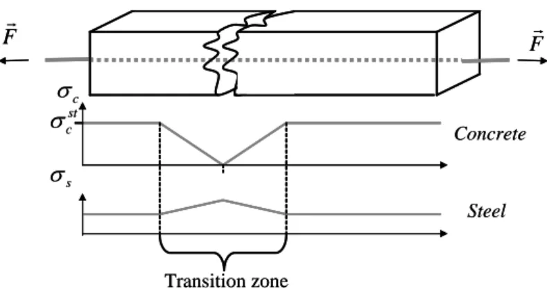
The validity of the models and more generally of the methodology for nonlinear computations developed to capture the mechanical behavior of concrete and reinforced concrete structures is generally obtained by comparing their performance with experimental results. The validation is performed on small-size specimens, where the elementary features of the models are tested (Ghavamian et al., 2003). When a satisfactory agreement is achieved in these initial configurations, more realistic computations can be imagined to evaluate the capacity of the models to reproduce real scale situations. But in these complex cases, regarding especially the dimensions of the problem, strong hypothesis has to be introduced to perform the numerical solution. When reinforced concrete structures are considered ((Parmar et al., 2014) or (Granger et al., 2001) for example), one of the most used hypotheses is to model the steel reinforcement as truss (or membrane) elements and to consider a no-slip (also called “perfect”) relation between steel and concrete. This no-slip relation is generally applied through cinematic relations between both models, using the shape functions of each element. But this hypothesis may have heavy consequences when the crack properties (spacing and openings) are studied, as the steel – concrete bond directly influences their evolutions ((Eligehausen et al, 1982), (Fib, 2000), (Gambarova et al, 2000), (Eurocode 2, 2007) or (Jason et al., 2013) for example). Indeed, cracking in reinforced concrete structures is generally driven by the stress distribution along the interface between steel and concrete. For example, in the case of a reinforced concrete tie, once the first crack appears in the weakest section, the concrete stress in the cracked zone drops to zero while the load is totally resisted by the steel reinforcement. The stresses are then progressively transferred from steel to concrete (Figure 1). This transition zone has an impact on the crack properties and is directly influenced by the steel–concrete interface (Eurocode 2, 2007). Taking into account these effects seems thus essential to predict correctly the cracking of reinforced concrete structures.
To understand the bond-slip mechanism, many experimental studies were carried out ((Lam and El-Lobody, 2005), (Loh et al., 2004), (Nie and Cai, 2001) or (Dancygier and Katz, 2012) for example) through various experimental setups. Analytical approaches were then attempted to fit the experimental results ((Bradford and Gilbert, 1992) on partial composite beam analysis or (Dezi et al., 1993) with the solution of the governing differential equation using the finite differential method). Numerical studies were also carried out, based on a double node concept to represent the relative slip between a concrete slab and a beam ((Gara et al., 2006), (Gattesco, 1999) and (Queiroz et al., 2009) among others).
Figure 1. Distribution of stresses in steel and concrete in a reinforced concrete tie after the first crack (
c and
sare the stresses in concrete and steel respectively, and
cst is the concrete strength).c Concrete Steel st c s Transition zone F F c Concrete Steel st c s Transition zone F F
3
This approach is easily applicable within the finite element formulation, but it increases significantly the number of degrees of freedom and also complexity in the mesh definition. Ngo and Scordelis (1967) proposed a spring element to relate concrete and steel nodes, associated to a linear constitutive law. To improve the description of the bond law, an interface element in 2D was introduced by Brancherie and Ibrahimbegovic (2009) or Dominguez et al. (2005) which enables the use of a nonlinear law. Dominguez (2005) and Ibrahimbegovic et al. (2010) finally proposed an embedded element in which the bond behavior is described through an enrichment of the degrees of freedom.
Even if these approaches propose a correct description of the bond mechanism between steel and concrete, they also have their own limits, especially in cases of real scale applications, such as meshing problems (explicit representation of 3D steel geometry), element direction or computation time which is very costly for large-scale applications (enriched elements like in (Dominguez, 2005)). That is why alternative solutions have been proposed ((Casanova et al., 2012) for example), first to represent the effects of the steel-concrete bond but also to be adapted to large scale applications (truss steel elements) with no need to explicitly mesh the steel-concrete interface (like in Dominguez et al., 2005 for example). Based on this principle, a new interface element is presented in this contribution. In a first part, the equations and the numerical implementation of the so-called “coaxial element” will be described. Then it will be verified by a comparison to an analytical solution on an academic problem. Finally, the model is compared with experimental results on a monotonic reinforced concrete tie.
2. Description of the bond slip model
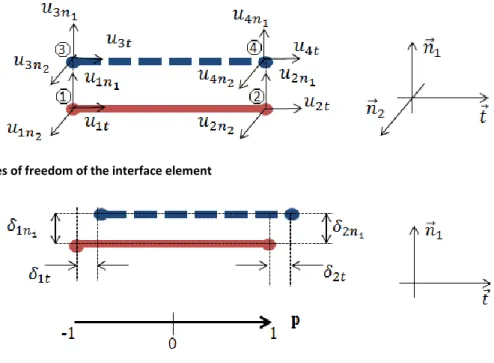
In this contribution, a new interface element is developed, based on the initial work from Casanova et al. (2012). It is a zero thickness four node element which relates each steel truss element with a segment superimposed with the steel element and perfectly bonded to the surrounding concrete (Figure 2). The perfect bond is done by imposing a similar displacement using the shape functions of the concrete element. Each node of the interface element has three degrees of freedom (translations). The following sections present the kinematics relations, the stress-slip relations and the numerical implementation.
2.1. Kinematics relations
As previously mentioned, the four node interface element is associated to 12 degrees of freedom
u
which can be written in the local direct reference frame as:
1, 11, 12, 2, 21, 22, 3, 31, 32, 4 , 41, 42
T
t n n t n n t n n t n n
u u u u u u u u u u u u u ( 1 )
4
Figure 3. Degrees of freedom of the interface element
Figure 4. Definition of the slip between steel and concrete in the interface element in the (t, n1) plane
t is the vector tangential to the direction of the steel truss element. n1 and n2 are chosen to represent a direct reference frame (Figure 3). The slip between steel and concrete node is then
computed using the following expression (Figure 4):
3 3 3 3
3 3 3 3 0 0 0 0 node I I u N u I I ( 2 ) with :
1, 11, 12, 2, 21, 22
T node t n n t n n ( 3 ) and 3 3 1 0 0 0 0 0 0 1 0 ; 0 0 0 0 0 0 1 0 0 0 I ( 4 )Considering the linearity of the slip along the interface element, the generalized slip
( )p
can be written as:
1
2 1 2 ( ) ( ) ( ) ( ) ( ) ( ) t n node n p p p B p B p p ( 5 ) with:5 1 3 2 3 ( ) 0.5(1 ) ( ) 0.5(1 ) B p p I B p p I ( 6 ) and 1 p 1 ( 7 )
Combining equations ( 2 ) and ( 5 ), it comes :
( )p
B p1( ) B p2( ) B p1( ) B p2( )
u B p u( )
( 8 )It is to be noted that the hypothesis of linearity for the slip is valid as linearity is supposed for the displacement.
2.2. Stresses and nodal forces in the interface element
The stresses
1 2 ( ) ( ) ( ) ( ) t n n p p p p in the interface element are direct functions of the slip
( )p
.In the tangential direction, the tangential stress t is computed from the tangential slip following the
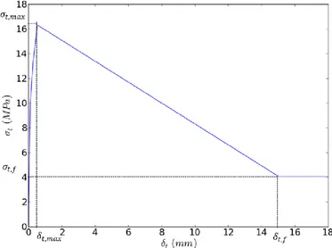
recommendations from Torre-Casanova et al. (2013) (bond stress – bond slip relation (Eligehausen et al., 1982) for example) (Figure 5 for the monotonic case):
( ) ( ( ))
t p f t p
( 9 )
The bond slip law f is especially driven by the maximum bond stress 𝜎𝑡,𝑚𝑎𝑥 and its corresponding tangential slip 𝛿𝑡,𝑚𝑎𝑥 and by the residual bond stress 𝜎𝑡,𝑓 and its corresponding tangential slip 𝛿𝑡,𝑓, which can be functions of the concrete cover (see (Torre-Casanova et al., 2013) for more details).
6
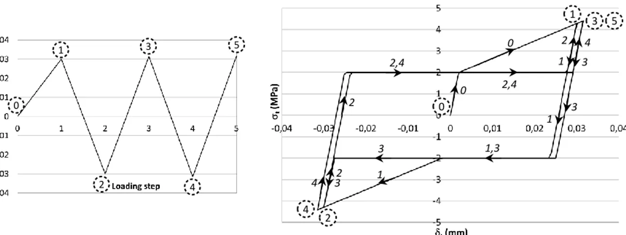
Figure 6. Evolution of the tangential bond stress as a function of the tangential slip (right) for an alternate loads in the pre-peak phase (left)
In cases of alternate loads, the bond slip law presented in Figure 5 has to be improved in order to take into account the unloading effects. Indeed, in case of unloading, the steel concrete bond is not reversible. Some authors experimentally studied the cyclic bond behavior, using for example pull-out tests or bending beams ((Eligehausen et al., 1983), (Spencer et al., 1982), (Soleymani Ashtiani et al., 2013) or (Campione et al., 2005)). After loading to any given stress level and at the onset of unloading, a sudden decrease of the bond stress is observed at almost constant slip, the slope being close to the initial slope of the loading elastic branch. Once a frictional limit is reached, a decrease of the slip is obtained at constant bond stress (friction). Finally, once the steel rib reaches undamaged concrete, the bond slip and bond stress follows a usual evolution. Following these experimental observations, a bond slip – bond stress law is proposed, including a non-reduced envelope (constant maximum bond stress with the number of cycles), as in (Kwak and Hwang, 2011). In this case, the bond slip – bond stress law is illustrated in the pre-peak phase in Figure 6. In addition to the bond parameters already mentioned in Figure 5, the unloading behavior requires the friction stress to be defined (equal to 2 MPa in the figure). This value is in agreement with the one experimentally obtained in (Torre-Casanova, 2012) or in (Torre-Casanova et al, 2012) for monotonic loads. It is to be noted that this value is difficult to calibrate as it is highly subjected to experimental dispersion.
In the normal directions, a linear relation is supposed between the stresses n1 and n2 and the
corresponding normal slip:
1 1 2 2 ( ) ( ) ( ) ( ) n n n n n p p k p p ( 10 )
For the sake of simplicity, the value of the normal stiffness kn is chosen high enough to be
representative of a perfect bond in the normal directions. Some improvements could be investigated in future works to take into account the effect of the bond slip behavior in the normal direction (for example unilateral contact if normal stress is in tension).
The nodal internal force vector
Finterface
in the local reference frame is then obtained by integrationalong the length of the element.
interface
1 2 3 4 T T T T T F F F F F ( 11 ) 1 0 2 3 4 5 1 0 2 3 4 5 0 0 1 1 1,3 1 2 2 2,4 2,4 2 3 3 3 3 4 47 with:
1
2 1 0 1 1 1 1 ( ) 2
t e n n F l F F A p dp F ( 12 )with le the length of the element and :
0 0 0 0 0 0 s s s d A d d ( 13 )
where ds is the steel diameter.
1
2 1 2 2 0 2 2 ( ) 2
t e n n F l F F A p dp F ( 14 )From the equilibrium of the forces between steel and concrete, it comes:
1
1
3 4 3 3 1 4 4 2 3 2 4 2 ; t t n n n n F F F F F F F F F F ( 15 ) 2.3. Numerical implementationThe model is implemented in the finite element code Cast3M (2014). A linearity of the stresses along the interface element is supposed for the numerical implementation. In this case, the generalized stresses can be written as functions of the stresses calculated at the positions of two Gauss points
1 11 12 2 21 22
T GP GP t GP n GP n GP t GP n GP n (Figure 7):
( )p
B p1( ) B p2( )Q
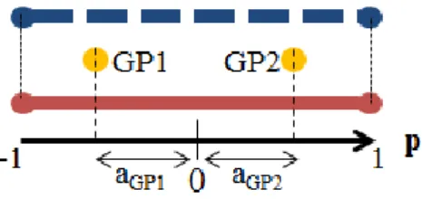
GP ( 16 ) where 1 1 1 2 1 1 2 2 2 ( ) ( ) ( ) ( ) GP GP GP GP B a B a Q B a B a ( 17 ) and 1 2 1 3 1 3 GP GP a a ( 18 )8
Figure 7. Positions of the Gauss points GP1 and GP2 in the interface element
Figure 8. Nodal forces in the global reference frame
After an analytical integration, it comes:
1 2 3 4 GP F F F CQ F F ( 19 ) 1 2 1 2 T T T T T C C C C C ( 20 ) 1 3 3 2 3 3 3 1 8 8 1 3 8 8 e e C l A I I C l A I I ( 21 )For the calculation of the nodal internal force vector in the global reference frame (Figure 8), a transformation matrix TLG is introduced from the local reference frame to the global one:
1 3 3 3 1 3 3 3 1 3 3 3 1 3 3 3 0 0 0 0 0 0 0 0 0 0 0 0 L G T T T T T ( 22 ) 1 2 1 1 2 1 2 . . . . . . . . . x t x n x n T y t y n y n z t z n z n ( 23 )
9 It comes:
1 2 3 4 L G GP global global F F F T CQ F F ( 24 )For the resolution, a Newton-Raphson scheme is used (Ma and May, 1986). The contribution of the interface element to the tangent stiffness matrixKinterfacen is computed using the equation:
interface n nT n global GP L G L G global F K T CQ T u u ( 25 )It supposes an update of the resolution matrix at each iteration, as a function of the position in the (t,
t) curve.
In the case of a linear evolution between the tangent bond stress and the slip, this matrix becomes constant and equal to:
interface 0 0 T global GP L G L G global F K T CQ T u u ( 26 ) 0 GP u is directly computed following the expression (in the local reference frame):
1 0 GP Q E node u u ( 27 ) with S S E S S and 0 0 0 0 0 0 t n n k S k k where : 0 t t t t k ( 28 )
Finally, it comes (in the global reference frame):
int T L G L G erface K T C E N T ( 29 )
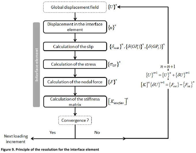
The steps for the resolution of the system are summarized in Figure 9. It is to be noted that the use of a constant matrix may induce convergence troubles, especially for the post-peak stage. Nevertheless, for the level of slip encountered in the applications, no problem was reported so far.
2.4 Model verification
In order to validate the numerical implementation of the interface element, its application to a rather simple reinforced concrete tension member is considered in the following, in the ideal situation where steel, concrete and steel-concrete bond behave elastically. To achieve this goal, a comparison with an analytical solution is performed.
10
Figure 9. Principle of the resolution for the interface element
Figure 10. Presentation of the test, the boundary conditions and loading
A reinforced concrete tie (length L equal to 1.15 m, square section Sc equal to 0.01m²), crossed by a
steel bar (diameter ds equal to 10 mm for a section Ss equal to 7.85 10-5 m2) is considered (Figure 10).
Concrete and steel are meshed with 50 elements in the length, using solid elements for concrete and truss elements for steel (Figure 11), with one concrete element in the section. At each end of the steel bar, one element is added to apply the boundary conditions (no displacement at one end) and the loading (imposed horizontal displacement at the other end) (Figure 10).
11
Figure 11. Concrete mesh for the analytical verification
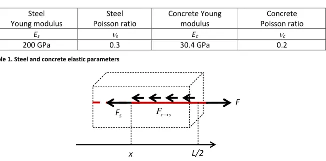
Steel Young modulus Steel Poisson ratio Concrete Young modulus Concrete Poisson ratio Es s Ec c 200 GPa 0.3 30.4 GPa 0.2
Table 1. Steel and concrete elastic parameters
Figure 12. Equilibrium of the steel bar between the loaded end and the abscise x
Steel and concrete are supposed to behave elastically, using the parameters given in Table 1. For this particular application, the steel-concrete bond between t and t in the tangential direction is
represented by a linear relation:
t kt t
( 30 )
with kt equal to 1011 Pa.m-1 (secant value for the bond slip – bond stress law as experimentally
reported in Torre-Casanova et al, 2013 for example).
To validate the implementation of the interface element and its ability to reproduce the effect of the steel-concrete bond, the numerical results are compared with an analytical solution. Considering the equilibrium of the steel bar between the loaded end and the abscissa x (Figure 12), the external force F applied at the end of the steel bar is balanced by the internal force Fs on the section and by the
bond force induced by concrete on the steel bar Fcs. It comes:
( ) ( ) c s s F x F x F ( 31 ) with F
F
s Fcs xL/2
12 ( ) ( ) ( ) s s s s s s s u x F x E S x E S x ( 32 )
with s( )x and u xs( )respectively the steel strain and steel displacement at x.
The bond force can be computed as follows:
/ 2 / 2 ( ) ( ) ( ( ) ( )) L L c s s t s t s c x x F x
d x dxd k
u x u x dx ( 33 )with u xc( )the concrete displacement at x.
The equilibrium of the force in concrete can be also written (considering the homogeneity of the concrete stress and strain in the section):
( ) ( ) 0 s c c F x F x ( 34 ) where ( ) ( ) ( ) c c c c c c c u x F x E S x E S x ( 35 ) and ( ) ( ) c s s c F x F x ( 36 )
c(x) stands for the concrete strain at x.
Using equations (32), (33), (34), it comes:
/ 2 ( ) ( ( ) ( )) L s s s s t s c x u x E S F d k u x u x dx x
( 37 )By a second derivation of the previous equation, combined to equations (35), (36) and (37), it comes:
3 3 ( ) ( ) s s u x u x a b x x ( 38 ) with 1 1 ( ) s t s s c c s t s s c c a d k S E S E d k F b S E S E ( 39 )
Hence, the evolution of the steel stress s is given by:
2 2 3 s s x ( 40 ) with a ; bEs
13
With the boundary conditions on the steel stress ( ) ( )
2 2
s s
s
L L F
S
and on the bond slip
(0) 0
t
(symmetry of the problem), we finally obtain for the steel stress, the concrete stress c and
the slip: 2 2 2 ( ) ( ) ( ) ( ) 2 ( ) ( ) ( 1) ( ) 2 ( ) ( ) ( ) ( ) ( ) 2 s s c c t s c s s F ch x x L S ch bE ch x x L ch Fsh x x u x u x L E S ch ( 41 )
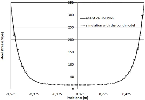
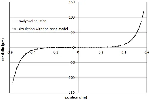
For the comparison between the analytical solution and the modelling, Figure 13 presents the evolution of the steel stress along the tie, for an imposed displacement of 0.5 mm corresponding to an applied force of 27.3 kN. A satisfactory agreement is obtained between the analytical solution and the modelling which validates the implementation of the model. Figure 14 gives the same comparison for the slip. Once again, a satisfactory agreement is obtained between the analytical solution and the modelling.
Qualitatively, the model is able to reproduce the transfer of stresses between the steel bar and concrete from the end of the tie to its center. The maximum of the stress transfer and of the bond slip is located at the end of the structure. In this sense, it is able to reproduce the effects related to the steel concrete bond as mentioned for example in (Eurocode 2, 2007).
14
Figure 14. Plot of the bond slip along the reinforcement according to the analytical and numerical solutions
3. Model validation on a reinforced concrete tie
In this section, the modelling using the steel-concrete bond element is compared with the experimental results from (Farra, 1995) on a monotonic reinforced concrete tie
3.1 Presentation of the test
The reinforced concrete tie experimentally studied in (Farra, 1995) has the same geometry as presented in Figure 10 (1.15m x 0.1m x 0.1m). Compared with the results presented for the verification, the mesh is here refined in the section (Figure 15). To reproduce the experimental behavior, the steel bar is represented using an elastic-plastic model with linear hardening. Concrete is modeled using a damage constitutive law developed in (Faria, 1998) and implemented in the finite element code Cast3M (2014). This constitutive law was chosen because it was successfully applied in previous works for structural applications ((Jason et al., 2013) for example). It includes damage in compression and in tension, which is regularized using the Hillerborg concept of fracture energy that guarantees a constant energy release, independently from the mesh size (Hillerborg et al., 1976). Parameters given in Table 2 and Table 3 are chosen, in agreement with the experimental data. Numerical responses in tension, compression and pure shear are illustrated in Figure 16.
. A random distribution of the tensile strength is added in order to localize the damage during loading (Figure 17). For the bond model, only the bond stress – bond slip law f has to be provided. A piecewise linear curve is chosen, following the recommendations from (Torre-Casanova et al., 2013). The parameters are given in Table 4. The resulting curve is illustrated in Figure 18.
15
Figure 15. Mesh of the reinforced concrete tie
Young modulus Poisson ratio Limit of elasticity Hardening slope
Es s se Eh
200 GPa 0.3 500 MPa 3245 MPa
Table 2. Steel parameters
Young modulus Poisson ratio Tensile strength Compressive
strength Fracture energy
Ec c ft fc Gf
30.4 GPa 0.2 2.6 MPa 56.9 MPa 150 N/m
Table 3. Concrete parameters
Figure 16. Uniaxial compression (left), tension (middle) and pure shear (right) responses for the concrete model
16
Bond stress (MPa) 2 10 13.2 21 2 2
Bond slip (mm) 0.002 0.1 0.25 0.765 1.5 1.8
Slope (Pa/m) 1012 8.2 1010 2.1 1010 1.5 1010 -1.3 109 0
Table 4. Parameters for the bond stress – bond slip law
Figure 18. Plot of the bond stress – bond slip law (monotonic evolution)
3.2. Results using the bond model
Figure 19 shows the evolution of the stress at the loaded end of the steel bar as a function of the mean concrete strain. The mean concrete strain is calculated from the relative displacement on a length L equal to 1m at the center of the tie.
The expected evolution is obtained including three main steps: a linear regime in which concrete and steel behave elastically, then a nonlinear regime where concrete is gradually damaged (active cracking) and finally a stage where the number of cracks in concrete does not evolve any more (stabilized crack). Some unloading zones are also observed in both experiment and modelling which correspond to the occurrence of a cross-wise damaged zone in the tie (“crack”). A satisfactory agreement is observed between experiment and modelling concerning the crack initiation and the envelope curve. As reported in (Farra, 1995), the “brittleness” of the experimental curve at the occurrence of the cracks is directly related to the experimental device and cannot be fully reproduced by the numerical solution.
17
Figure 19. Plot of the stress in the reinforcement as a function of the mean strain in concrete according to the numerical solution and the experiment
Moreover, on this type of application (reinforced concrete tie), the occurrence of the cracks is directly related to the spatial distribution of the tensile strength and may thus be different between two similar experiments (as observed in (Farra, 1995)). That is why a perfect agreement cannot be reached between experiment and modelling. Figure 20 illustrates the evolution of the mean crack opening as a function of the mean concrete strain. In the modelling, the crack opening is calculated from the evolution of the horizontal relative displacement. For the calculation of the mean opening, a crack is taken into account once it has reached a value greater than 50 m. A satisfactory agreement is obtained, especially during the stabilized cracking phase. A correct number of cracks (five) is predicted by the model. As already observed in Figure 19, differences in the evolution of the mean crack opening are partly related to the random distribution of the tensile strength.
Figure 20. Plot of the mean crack opening as a function of the mean concrete strain according to the numerical solution and the experiment
18
Figure 21. Plot of the crack openings as a function of the mean concrete strain according to the numerical solution (dashed curves) and the experiment (full curves)
Finally, local quantities are investigated. Figure 21 provides the evolutions of each crack opening with the mean concrete strain. In both experimental and numerical results, the occurrence of a new crack is responsible for the decrease in the openings of the other cracks.
The number of the cracks yielded by the proposed numerical approach (five at the end of the loading) and their openings are in a quite satisfactory agreement with experiment. It thus validates the ability of the proposed bond model to represent the cracking behavior of this reinforced concrete tie.
3.3. Discussion on the bond effect
In this section, the interest of the bond model compared with the “perfect” no-slip relation hypothesis is discussed. To this aim, a second computation is performed on the reinforced concrete tie where each steel node has the same displacement as the concrete element in which it is included (zero slip). This so-called “perfect” bond is applied using additional cinematic relations. It is to be noted that the random distribution of the tensile strength is particularly useful in this case as it avoids a homogeneous damage field along the reinforced concrete tie (excepted for the end of the tie) (Figure 22).
Figure 22. Example of a damage distribution obtained without the random distribution of the tensile strength (no-slip perfect bond)
19
Figure 23 illustrates the evolution of the steel stress at the loaded end of the bar as a function of the mean strain in concrete. As already reported in (Richard et al., 2011) for example, a smother behavior is obtained when a no-slip relation is considered. In this case, the no-slip relation only reproduces the envelope behavior. Nevertheless, the time of first cracking is the same and the evolution up to the end of the loading remains similar compared with the bond model and to the experiment.
Figure 24 gives the evolution of the mean crack opening as a function of the mean strain in concrete. Compared with the global behavior, more significant differences appear. For a given mean strain in concrete, the mean crack opening is clearly underestimated by the no-slip “perfect” relation compared with the experiment or the bond model.
Figure 23. Plot of the steel stress as a function of the mean concrete strain according to the numerical solutions (using the bond model or the no-slip “perfect relation) and the experiment
Figure 24. Plot of the mean crack opening as a function of the mean concrete strain according to the numerical solutions (using the bond model or the no-slip “perfect relation) and the experiment
20
For the same loading, more cracks appear with the no-slip “perfect” relation with smaller openings. This is partly related to a wrong representation of the stress transfer between steel and concrete. This effect is underlined in Figure 25. Contrary to the experiment and to the situation in which the bond model is used, the no-slip relation induces the simultaneous occurrence of cracks, especially during the initiation. As a consequence, the mean crack opening is significantly lower than the experimental value. At the end of the loading (stabilized cracking phase), six cracks are modelled while five cracks are experimentally observed. For a mean concrete strain equal to 1.4 0/
00, the
modelled maximum crack opening using the no-slip relation is 275 m. The corresponding experimental value is 324 m while the value obtained with the bond model is 298 m. The bond model is thus clearly more appropriate to describe the local behavior of the reinforced concrete structure.
Figure 25. Plot of the crack opening as a function of the mean concrete strain according to the numerical solution, using the no-slip “perfect relation
Figure 26. Damage distributions in concrete at the end of the loading using the no-slip “perfect” relation (left) or the bond model (right)
21
Finally, Figure 26 illustrates the damage distributions using the no-slip relation (left) and the bond model (right). The same tendency is observed with a higher number of heavily-damaged zones (indirectly representing crack positions) when the no-slip relation is considered. In this case, one can also notice a concentration of damage at each end of the structure that reaches the whole section. On the contrary, with the bond model, the damage is only localized around the steel bar.
4. Conclusions
A new interface element has been proposed to take into account the effect of the steel-concrete bond. It is adapted to large scale applications as it has been developed to relate 1D truss elements for steel to 3D concrete elements, even in a case of non-coincident meshes. Its implementation was verified by comparison to an analytical solution in the case of a simplified reinforced concrete tie with elastic materials. The model is able to reproduce the effects of the steel-concrete bond with the stress transfer between steel and concrete during loading and after crack occurrence. It was also validated on a reinforced concrete tie by a comparison to experimental results. A satisfactory agreement was observed both on global (steel stress – mean strain curve) and local results (evolution of the local and mean crack openings). It thus succeeded in describing the behavior of this reinforced concrete structure, contrary to the no-slip “perfect” relation that induced a higher number of cracks. In this case, including the bond behavior through the proposed model enables to obtain more realistic results concerning the crack properties (crack opening and spacing).
Future work will concern the validation of the cyclic part of the model that has been implemented but not totally validated with the concrete tie (only partly during the partial unloading). To this aim, more complicated structures like cyclic shearing wall with more complex crack pattern could be investigated.
References
Bradford, M.A. and Gilbert, R.I. (1992), “Composite beams with partial interaction under sustained loads”, ASCE Journal of Structural Engineering, Vol. 118 No. 7, pp. 1871-1883
Brancherie, D. and Ibrahimbegovic, A. (2009), “Novel anisotropic continuum-discrete model capable of representing localized failure of massive structures. Part I: Theoretical formulation and numerical implementation”, Engineering Computations, Vol. 26, pp. 100-127
Campione, G., Cucchiara, C., La Mendola, L. and Papia, M. (2005), “Steel–concrete bond in lightweight fiber reinforced concrete under monotonic and cyclic actions”, Engineering Structures, Vol. 27 No. 6, pp.881-890
Casanova, A., Jason, L. and Davenne, L. (2012), “Bond slip model for the simulation of reinforced concrete structures”, Engineering Structures, Vol. 39, pp.66-78
Cast3M, http://www-cast3m.cea.fr, 2014
Dancygier, A.N. and Katz, A. (2012), “Bond over direct support of deformed rebars in normal and high strength concrete with and without fibers”, Journal of Materials and Structures, Vol. 45, pp.265-275 Dezi, I., Ianni, C. and Tarantino, A.M. (1993), “Simplified creep analysis of composite beams with flexible connectors”, ASCE Journal of Structural Engineering, Vol. 119 No. 5, pp. 1484-1497
22
Dominguez, N., Brancherie, D., Davenne, L. and Ibrahimbegovic, A. (2005), “Prediction of crack pattern distribution in reinforced concrete by coupling a strong discontinuity model of concrete cracking and a bond slip of reinforcement model”, Engineering Computations, Vol. 22, pp. 558-582 Dominguez, N. (2005), “Etude de la liaison-acier enter l’acier et le béton: de la modélisation du phénomène à la formulation d’un élément enrichi "Béton Armé"”, PhD thesis, Ecole Normale Supérieure de Cachan
Eligehausen, R., Popov, E.P. and Bertoro, V.V. (1982), “Hysteretic behaviour of reinforcing deformed hooked bars in reinforced concrete joints”, Proceedings of the 7th European conference of
Earthquake Engineering, Athens, Vol.4, pp. 171-178
Eligehausen, R., Popov, E.P. and Bertoro, V.V. (1983), “Local bond stress slip relationships of deformed bars under generalized excitation”, Report 82/23, Earthquake Engineering Research Center, University of California, Berkeley, 169 pages
Eurocode 2 (2007), « Calcul des Structures en béton », NF-EN-1992
Faria, R., Oliver, J. and Cervera, M. (1998), “A strain-based plastic viscous-damage model for massive concrete structures”, International Journal for Solids and Structures, Vol. 35 No. 14, pp. 1533–1558 Farra, B. (1995), “Influence de la résistance du béton et de son adhérence avec l’armature sur la fissuration”, PhD Thesis, Ecole Polytechnique Fédérale de Lausanne
Fib (2000), “Bond of reinforcement in concrete”, Bulletin n.10, State-of-Art report, Task group “bond models” , Convener Ralejs Tepfers, 42 pages
Gambarova, P.G., Plizzari, G., Rosati, G.P, Russo, G. (2000), “Bond mechanics including pull-out and splitting failures, State-of-Art report on “bond of reinforcement in concrete”, Chapter 1 of fib bulletin N. 1, edited by fib Task Group “bond models” chaired by Tepfers, pages 1-98
Gara, F., Ranzi, G. and Leoni, G. (2006), “Displacement-based formulations for composite beams with longitudinal slip and vertical uplift”, International Journal of Numerical Methods in Engineering, Vol. 65 No. 8, pp. 1197-1220
Gattesco, N. (1999), “Analytical modeling of non-linear behavior of composite beams with deformable connection”, Journal of Constructional Steel Research, Vol. 52 No. 2, pp. 1995-2018 Ghavamian, S., Carol, I. and Delaplace, A. (2003), “Discussions over MECA project results”, Revue Française de Génie Civil, Vol. 7 No. 5, pp. 543-581
Granger, L., Rieg, C.Y., Touret, J.P., Fleury, F., Nahas, G., Danisch, R., Brusa, L., Millard, A., Laborderie, C., Ulm, F., Contri, P., Schimmelpfennig, K., Barre, F., Firnhaber, M., Gauvain, J., Coulon, N., Dutton, L.M.C and Tuson, A. (2001), “Containment Evaluation under Severe Accidents (CESA): synthesis of the predictive calculations and analysis of the first experimental results obtained on the Civaux mock-up”, Nuclear Engineering and Design, Vol. 209, pp. 155–163
Hillerborg, A., Modeer, M. and Peterson, P.E. (1976), “Analysis of crack formation and crack growth in concrete by means of fracture mechanic and finite elements”, Cement and Concrete Research, Vol. 6, pp. 773–782
23
Ibrahimbegovic, A., Boulkertous, A., Davenne, L. and Brancherie, D. (2010), “Modeling of reinforced concrete structures providing crack spacing based on XFEM, EDFEM and novel operator split solution procedure”, International Journal of Numerical Methods in Engineering, Vol. 83, pp. 452-481
Jason, L., Torre-Casanova, A., Davenne, L. and Pinelli, X. (2013), “Cracking behavior of reinforced concrete beams. Experiment and simulations on the numerical influence of the steel-concrete bond”, International Journal of Fracture, Vol. 180 No. 2, pp. 243-260
Kwak, H.G. and Hwang, J.W. (2011), “Nonlinear finite element analysis of a steel concrete composite beam under cyclic loads considering interface slip effects”, Engineering letter, Vol. 19 No. 3, pp. 249-254
Lam, D. and El-Lobody, E. (2005), “Behavior of headed stud shear connectors in composite beam”, Journal of Structural Engineering, Vol. 131 No. 1, pp. 96-919
Loh, H.Y., Uy, B. and Bradford, M.A. (2004), “The effects of partial shear connection in the hogging moment regions of composite beams. Part I: Experimental study” Journal of Constructional Steel Research, Vol. 60 No. 6, pp. 897-919
Ma, S. Y. A. and May, I. M. (1986), “The Newton-Raphson method used in the non-linear analysis of concrete structures”, Computers and Structures, Vol. 24 No. 2, pp.177-185
Ngo, D. and Scordelis, A.C. (1967), “Finite element analysis of reinforced concrete beams”, ACI Journal, Vol. 64, pp. 152-163
Nie, J. and Cai, C.S. (2001), “Steel-concrete composite beams considering shear slip effects”, Journal of Structural Engineering, Vol. 127 No. 4, pp. 359-366
Parmar, R.M., Signh, T., Thangamani, I., Trivedi, N. and Singh, R.K. (2014), “Over-pressure test on BARCOM pre-stressed concrete containment”, Nuclear Engineering and Design, Vol. 269, pp.177-183 Queiroz, F.D, Queiroz, G. and Nethercot, D.A. (2009), “Two dimensional FE model for evaluation of composite beams. I: Formulation and validation”, Journal of Constructional Steel Research, Vol. 65 No. 5, pp. 1055-1062
Richard, B., Ragueneau, F., Adelaïde, L. and Cremona, C. (2011), “A multi-fiber approach for modeling corroded reinforced concrete structures”, European Journal of Mechanics - A/Solids, Vol. 30 No. 6, pp. 950-961
Soleymani Ashtiani, M., Dhaka, R.P., Scott, A. N. and Bull D. K. (2013), “Cyclic beam bending test for assessment of bond slip behavior”, Engineering Structures, Vol. 56, pp. 1684-1697
Spencer, R.A., Panda; A.K. and Mindess, S. (1982), “Bond of deformed bars in plain and fiber reinforced concrete under reversed cyclic loading”, International Journal of Cement Composite and Lightweight Concrete, Vol. 4 No. 1, pp.3-17
Torre-Casanova, A., Jason, L., Davenne, L. and Pinelli, X. (2013), “Confinement effects on the steel-concrete bond strength and pull-out failure”, Engineering Fracture Mechanics, Vol. 97, pp. 92-104
24
Torre-Casanova, A. (2012), « Prise en compte de la liaison acier-béton pour le calcul de structures industrielles », PhD Thesis, Ecole Normale Supérieure de Cachan