HAL Id: hal-01636652
https://hal.archives-ouvertes.fr/hal-01636652
Submitted on 7 Sep 2018
HAL is a multi-disciplinary open access
archive for the deposit and dissemination of
sci-entific research documents, whether they are
pub-lished or not. The documents may come from
teaching and research institutions in France or
abroad, or from public or private research centers.
L’archive ouverte pluridisciplinaire HAL, est
destinée au dépôt et à la diffusion de documents
scientifiques de niveau recherche, publiés ou non,
émanant des établissements d’enseignement et de
recherche français ou étrangers, des laboratoires
publics ou privés.
Increasing Reliability of a TSCH Network for the
Industry 4.0
Pascale Minet, Ines Khoufi, Anis Laouiti
To cite this version:
Pascale Minet, Ines Khoufi, Anis Laouiti. Increasing Reliability of a TSCH Network for the Industry
4.0. 16th IEEE International Symposium on Network Computing and Applications (NCA 2017), Oct
2017, Boston, United States. �10.1109/NCA.2017.8171344�. �hal-01636652�
Increasing Reliability of a TSCH Network
for the Industry 4.0
Pascale Minet
∗, Ines Khoufi
∗and Anis Laouiti
†∗Inria, 2 rue Simone Iff, CS 42112, 75589 Paris Cedex 12, France. Email: [email protected], [email protected] †SAMOVAR, T´el´ecom SudParis, CNRS, Universit´e Paris-Saclay, 9 rue Charles Fourier 91011 Evry, France
Email: [email protected]
Abstract—Time Slotted Channel Hopping (TSCH) networks are emerging as a promising technology for the Internet of Things and the Industry 4.0 where ease of deployment, reliability, short latency, flexibility and adaptivity are required. Our goal is to improve reliability of data gathering in such wireless sensor networks. We present three redundancy patterns to build a reliable path from a source to a destination. The first one is the well-known two node-Disjoint paths. The second one is based on a Triangular pattern, and the third one on a Braided pattern. A comparative evaluation is carried out to analyze the reliability achieved, the number of failures tolerated, the number of message copies generated and the energy consumed by each node to ensure that at least one copy of the message is delivered to the destination. These results are validated by simulations.
I. CONTEXT AND MOTIVATION
By the year 2020, it is expected that the number of connected objects will exceed several billions devices. These objects will be present in everyday life for a smarter home and city as well as in future smart factories that will revolutionize the industry organization. This is actually the expected fourth industrial revolution, more known as Industry 4.0 [11]. In which, the Internet of Things (IoT) is considered as a key enabler for this major transformation [8]. IoT will allow more intelligent monitoring and self-organizing capabilities than traditional factories. As a consequence, the production process will be more efficient and flexible with products of higher quality.
Several standards have been designed for industrial wireless sensor (IoT) networks such as WirelessHart and ISA100. Both of them are based on the IEEE 802.15.4 standard for the lower layers. More recently, Time Slotted Channel Hopping (TSCH) which is specified in amendment e of the IEEE 802.15.4 standard [9], uses a time slotted medium access operating on several channels simultaneously. In addition, radio perturba-tions are mitigated by frequency hopping. TSCH supports star and mesh topologies, as well as multi-hop communication. It has been designed for process automation, process control, equipment monitoring and more generally the Internet of Things. It is a candidate technology for the Industry 4.0. In fact, Industry 4.0 will use more and more the on-demand man-ufacturing in a highly fexible and widespread environment. Different supply chains located in various regions need to coordinate their actions in a real-time basis with high fidelity. The IoT communicating in a wireless manner will play a major role to achieve this target. However, the strong requirements in
terms of short latency and high reliability of such applications are obstacles to its penetration in the Industry 4.0.
How to improve the reliability of an end-to-end commu-nication, while meeting a short latency and minimizing the overhead incurred? This is the focus of this paper which is organized as follows. Section II presents related work and po-sitions our contribution. In Section III, we define the problem we deal with. In Section IV, we introduce three redundancy patterns and describe how they are used in a TSCH network. For each pattern, we evaluate its reliability, its impact on the TSCH schedule, the bandwidth and the energy consumed by an end-to-end transmission in Section V. These performance results are computed theoretically and by means of simulations with NS3. We discuss the advantages and drawbacks of each solution. Finally, we conclude in Section VI.
II. RELATED WORK
TSCH provides a multichannel slotted medium access ruled by a periodic schedule. This schedule is repeated every slot-frame. A slotframe consists of a set of cells, each cell is identified by a (time slot offset, channel offset) pair. The size of a timeslot (e.g. 10 ms by default) allows the transmission of a point-to-point frame and its immediate acknowledgment. The schedule defines for each cell the nodes allowed to transmit and those that should receive. The channel offset is translated into a physical channel depending on the channel hopping sequence of the TSCH network. Channel hopping allows the TSCH to increase its robustness against external perturbations of the radio signal. There are two types of cells in a slotframe. The dedicated cells provide a collision-free access (i.e. multichannel TDMA) and are used to transmit data. Shared cells allow several transmitters to compete for the medium access based on CSMA/CA, with possible collision. They are used to broadcast messages and to advertise the TSCH network. The scheduled MAC access allows the nodes to save energy by sleeping whenever they are not involved in a communication. More details can be found in [4], [9].
There are several studies evaluating the performances of a TSCH network. They vary in the performance evaluated (e.g. average delivery rate [3], average or upper bound on delivery delays and average energy consumed by an end-to-end transmission [16]) and the tools used for this purpose (e.g. simulator for [3], analytical model, Network calculus for [7], measures on real networks for [14]).
NS2 simulation results reported in [3] show that a TSCH network outperforms a classical 802.15.4 network, both in beacon-enabled and non-beacon enabled modes, in terms of delivery ratio, energy consumed and delivery delays for a star topology with 20 to 120 nodes. The unreliability of wireless links is taken into account in a few papers, like in [14], where the packet error rate on each link is used to evaluate the average delivery time and the average energy consumption. To improve network reliability, an approach consists in avoiding the occurrence of link/node failures by selecting the most reliable intermediate nodes to build the end-to-end path. The reliability can take into account the Packet Delivery Rate (PDR) on the link considered, the energy of the candidate node, the SNR, etc. Examples are given in [13] for a clustered WSN. In the RPL routing protocol [15], the objective function determines the rank of a node. Various objective functions have been defined. The simplest one depends only on the distance to the sink. This approach decreases the probability of a failure occurring while a message is transiting on the path to the destination. However, it is unable to tolerate the failure of any intermediate node in this path.
The oldest technique used to tolerate one node or link failure in an end-to-end transmission consists in building two node-or-edge-disjoint paths [10] from the source to the destination. This technique will be analyzed in this paper. In [6], the authors propose Leapfrog Collaboration that operates with the RPL protocol in a TSCH network. We will present the associated redundancy pattern and analyze it.
III. PROBLEM STATEMENT
In this paper, we adopt the following assumptions:
• A1 The latency for the end-to-end message delivery, the
reliability and the node power autonomy constraints are given by the industrial application considered.
• A2 This application is supported by a TSCH network:
each transmission starts at a slot beginning. The slot size allows the transmission of one packet and its immediate acknowledgment when this packet is sent point-to-point.
• A3 Let S be any sensor node that has a message to
transmit to the sink, denoted D.
• A4 The TSCH network is assumed to be connected and
a routing protocol like RPL [15] is in charge of building the primary path between S and D. In other words, each node N has a def ault parent that is a 1-hop neighbor with a rank strictly smaller than N . The function used to compute the rank is defined in RPL. The simplest one is the distance to the sink, distance expressed in the number of hops. The primary path is formed according to the relationship ”has for default parent”. In addition, all 1-hop neighbor nodes of N with a rank strictly smaller than itself are called potential parents.
• A5 There is a schedule that ensures that the end-to-end
delivery time of a message from S to D meets the latency required by the application, in the absence of node/link failure.
• A6 The reliability of each wireless link is periodically
evaluated. The reliability of the link from Ni to
Nj is a function of the reception rate evaluated
in a sliding window; at iteration t, it is given by: RN i,N j(t) = α
number of msg f rom Ni received by Nj
number of msg sent by Ni to Nj
+(1 − α)Ri,j(t − 1)
where a large value of the constant α, with 0 ≤ α ≤ 1, means a fast forgetting of the past.
With these assumptions, we want to solve the following problem: Assuming the existence of a primary path, built by the routing protocol, between a source S and a destination D, how to improve the reliability of an end-to-end transmission from S to D in a TSCH network while meeting a short delivery delay and minimizing the overhead incurred?
The notations adopted in this paper are given in Table I. TABLE I: Notations.
Name Meaning
S Source node, also denoted N0
D Destination node, also denoted N2L−1
Ni Intermediate node, i ∈ [1, 2(L − 1)]
RN i,N j Reliability of the link from Nito Nj
L Length of the path expressed as the number of hops
between the source and the destination
E(N ) Energy consumed by node N
ET x(msg) Energy consumed to transmit a message
ET x(ack) Energy consumed to transmit an acknowledgment
ERx(msg) Energy consumed to receive a message
ERx(ack) Energy consumed to receive an acknowledgment
dp(N ) Default parent of node N
ap(N ) Alternate parent of N
dc(N ) Default child of N , N is default parent of dc(N )
ac(N ) Alternate child of N , N is alternate parent of ac(N )
IV. REDUNDANCY PATTERNS
After having selected the most reliable components, as in [13], the only mean to increase reliability consists in introducing redundancy and manage it according to either a masking approach or a detection-recovery approach. In a masking approach, the error is masked as long as the number of faults occurring is smaller than or equal to the number of faults tolerated. In a detection-recovery approach, the error, if any, must be detected before being recovered. In other words, the processing done depends on the effective occurrence of an error, whereas in a masking approach, the processing is independent. An example of a detection-recovery technique is given by Automatic Repeat reQuest (ARQ) [5]. It is an error-control method for data transmission that uses acknowledgements and timeouts. Two disjoint paths where each message is systematically transmitted on the two disjoint paths is an example of masking technique. In this section, we introduce three redundancy patterns to improve the reliability of an end-to-end transmission from S to D.
A. The Disjoint-path pattern
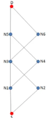
The first solution consists in building an alternate path to the primary path between S and D, such that these paths share no intermediate node, in order to tolerate one failure of any intermediate node. These two paths are said node-disjoint. The source node sends a copy of its message on the
primary path and another copy on the secondary path. Each copy follows its path independently. In the absence of failure, the destination receives two copies of the same message. It delivers the message arrived first and discards the copy arrived later. Such a pattern is called Disjoint-path pattern. Figure 1 depicts a primary path made of intermediate nodes with an odd identifier, whereas in the secondary path, the intermediate nodes have an even identifier.
Fig. 1: Disjoint-path pattern.
To build the two node-disjoint paths requires two iterations of the Dijkstra’s algorithm [10]. The main advantage of this solution lies in the fact that only the source and the destination have to manage the path redundancy which is kept totally transparent to any intermediate node belonging either to the primary path or to the secondary one. In addition, this approach being a masking one, the node behavior that has to be scheduled does not depend on the effective occurrence of a link/node failure.
B. Triangular pattern
The Triangular pattern has been initially designed for the MOLSR Multicast routing protocol [12] based on the unicast routing protocol OLSR [1]. Its goal was to increase the reliability of the multicast routing tree. The basic pattern is based on the triangle formed by a node N , its alternate parent denoted ap(N ) and its grandparent denoted dgp(N ), as depicted in Figure 2. Hence, if a link or node failure occurs on the primary path, depicted in red, the alternate path depicted in green and using the alternate node of the failed primary node is used to deliver the message.
Fig. 2: Basic triangle.
Each node N on the primary path, except the destination, has one default parent dp(N ) and one alternate parent ap(N ). Each alternate parent M has a triangular parent denoted tp(M ) on the primary path. More particularly, any node N on the primary path selects as alternate parent ap(N ) a potential parent that has its default grand parent dgp(N ) as potential parent, whereas M = ap(N ) selects dgp(N ) as its triangular
parent tp(M ), as illustrated in Figure 2. In Figure 3, node N 1 selects node N 4 as its alternate parent, and N 4 selects N 5 as its triangular parent. In the Triangular pattern, the end-to-end transmission is performed as follows. Each node on the primary path sends its message to both its default parent and its alternate parent, whereas each alternate parent sends the message only to its triangular parent.
Fig. 3: Reliable path based on a Triangular pattern. Each node N in the TSCH network maintains its set of potential parents. We distinguish two cases:
• If N is on the primary path and is not the destination (i.e. N is a default parent or the source), N should select a default parent and an alternate parent among its potential parents. As a consequence, N is required to know its potential parents as well as its default grandparent with its one-hop neighbors.
• If M is an alternate parent of N , M should select its triangular parent among its potential parents, which is the node default grandparent of N . M is only required to know its potential parents.
The algorithm is very simple. In addition, similarly to the Disjoint-path pattern, the schedule does not depend on the presence or absence of a link or node failure. All the transmissions are systematically scheduled.
C. Braided pattern
The Braided pattern is an extension of the Triangular pat-tern, in which an alternate path has been built with the alternate parents as intermediate nodes. It can also be seen as an extension of the Disjoint-path pattern where they are connected by multiple cross links, enabling multiple possibilities of going from one path to the other. Hence, the name of the pattern. This redundancy pattern is defined in [6], where it is part of the Leapfrog Collaboration running in collaboration with the RPL routing protocol in a TSCH network. It proceeds as follows. Similarly to the Triangular pattern, each node N on the primary path, except the destination, selects as its alternate parent one node among its potential parents that has for potential parent the default grand parent of N , as depicted in Figure 2. For instance, in Figure 4, node N 3 selects node N 6 as its alternate parent. There is an additional condition: the alternate parents of nodes in the primary path should form
an alternate path, (e.g. the path S, N2, N4, N6, D).
Each packet is sent twice by the source and any intermediate node: once to the default parent and once to the alternate parent. At each level in the routing tree maintained by RPL, each node forwards only once the message received, to each of its two parents, even if it has received several copies. Such copies are discarded.
Fig. 4: Reliable path based on a Braided pattern.
V. COMPARATIVE EVALUATION
Industry 4.0 is looking for an IoT exhibiting high perfor-mance in terms of reliability, latency and energy. That is why, in this section we compare the performances obtained by each redundancy pattern previously presented.
A. Reliability
The three redundancy patterns presented, namely the Disjoint-path pattern, the Triangular pattern and the Braided pattern tolerate only one link failure or only one node failure. None of them is able to tolerate the failure of:
• either two nodes having the same rank in the pattern considered, like for instance N3and N4.
• or two links with either the source, like for instance SN1
and SN2, or the destination like for instance N5D and
N6D.
However, the reliability of an end-to-end transmission provided by each pattern differs, as shown hereafter. To be able to quantitatively evaluate the increase in reliability brought by each redundancy pattern, we start by computing the reliability of the single path (i.e. the primary path) from S to D. This pattern is called ”No Redundancy” pattern and will be used as a reference. Numerical values of the reliability provided by each pattern studied are given in Table II for various link reliabilities. For a sake of simplicity, we assume that all nodes on the primary path have an odd identifier, whereas alternate nodes have even identifiers. In addition, we assume that at the same level in the routing tree, the primary node has an identifier smaller than the alternate node. Figures 1, 3 and 4 illustrate such a notation for the Disjoint-path, the Triangular and the Braided patterns, respectively. In this section, we evaluate the reliability of each pattern both theoretically and by simulations with NS3.
1) Theoretical evaluation of the reliability: a) Disjoint-path pattern.
The reliability of an end-to-end transmission, denoted RDisjointover two node-disjoint paths, denoted P rim for the
primary one and Sec for the secondary one, is the probability of a successful end-to-end transmission: the message sent by S is delivered to the destination D. D may successfully receive the message on the primary path, the secondary one or both of them. Hence, RDisjointis equal to the probability that P rim,
Sec or both delivers the message from S to D. We have: RDisjoint = RP rimS Sec = RP rim+ RSec− RP rimT Sec.
Assuming that link and node failures on the primary path do not depend on those occurring on the secondary path, we get:
RDisjoint= RP rim+ RSec− RP rim∗ RSec,
with RP rim=Qi∈P rimRi,dp(i)and RSec=Qi∈SecRi,dp(i),
since the reliability of a path is equal to the product of the reliability of each link composing this path.
b) Triangular pattern
We now focus on the Triangular pattern. The reliability of the Triangular pattern, denoted RT riangular, is given by the
probability that D receives the message transmitted by S. D may receive it from its default child (i.e. node N5in Figure 3),
its alternate child (i.e. node N6 in Figure 3), or from both of
them. We denote topN the probability that node N receives
the message sent by S. With this notation the reliability of the Triangular pattern depicted in Figure 3 is given by:
RT riangular= RN 5,D∗ topN 5+ RN 6,D∗ topN 6− Probability
that both N5 and N6 receive the message. Assuming that
failures on the primary path and on the alternate paths are independent, we get:
RT riangular = RN 5,D∗ topN 5+ RN 6,D∗ topN 6− RN 5,D∗
topN 5∗ RN 6,D∗ topN 6.
The default child of D (i.e. node N5in Figure 3) may receive
the message either from its default child (i.e. node N3 in
Figure 3), its alternate child (i.e. node N4in Figure 3), or from
both of them. However, an alternate parent, unlike a primary parent, has only one possibility to receive the message from S: it is via the node that selects it as its alternate parent, as depicted in green in Figure 5, where N6may receive only from
N3, whereas a primary parent like N5 has two possibilities
depicted in red.
Fig. 5: Two possibilities for a primary parent and only one possibility for an alternate parent in a Triangular pattern.
We proceed by successive iterations, progressing from the destination D downwards to the source S. Finally, we get the following system of equations:
RT riangular = RN 5,D∗ topN 5+ RN 6,D∗ topN 6
−RN,5D∗ topN 5∗ RN 6,D∗ topN 6
topN 6 = RN 3,N 6∗ topN 3
topN 5 = RN 3,N 5∗ topN 3+ RN 4,N 5∗ topN 4
−RN 3,N 5∗ topN 3∗ RN 4,N 5∗ topN 4
topN 4 = RN 1,N 4∗ topN 1
topN 3 = RN 1,N 3∗ topN 1+ RN 2,N 3∗ topN 2
−RN 1,N 3∗ topN 1∗ RN 2,N 3∗ topN 2
topN 2 = RSN 2
topN 1 = RSN 1
This system of equations can be generalized to any triangular pattern whose length of the primary path is L:
RT riangular = RN 2L−3,D∗ topN 2L−3+ RN 2L−2,D∗ topN 2L−2
−RN 2L−3,D∗ topN 2L−3∗ RN 2L−2,D∗ topN 2L−2 topN 2L−2j = RN 2L−2j−3,N 2L−2j∗ topN 2L−2j−3 topN 2L−2j−1 = RN 2L−2j−3,N 2L−2j−1∗ topN 2L−2j−3 +RN 2L−2j−2,N 2L−2j−1∗ topN 2L−2j−2 −RN 2L−2j−3,N 2L−2j−1∗ topN 2L−2j−3 ∗RN 2L−2j−2,N 2L−2j−1∗ topN 2L−2j−2 topN 2 = RSN 2 topN 1 = RSN 1with j ∈ [1, L − 2]. (1) c) Braided pattern
The reliability of the Braided pattern is also given by the probability that D receives the message transmitted by S. We proceed similarly to the Triangular pattern. The only difference comes from the fact that in the Braided pattern, the alternate parents, like the primary parents have two possibilities to receive the message sent by S, as depicted in Figure 6 in red for the primary parent N5 and in green for the alternate
parent N6. We proceed by successive iterations, progressing
from the destination D downwards to the source S.
Fig. 6: Two possibilities for a primary parent and an alternate parent in a Braided pattern.
Finally, we get the following system of equations:
RBraided = RN 5,D∗ topN 5+ RN 6,D∗ topN 6
−RN,5D∗ topN 5∗ RN 6,D∗ topN 6
topN 6 = RN 3,N 6∗ topN 3+ RN 4,N 6∗ topN 4
−RN 3,N 6∗ topN 3∗ RN 4,N 6∗ topN 4
topN 5 = RN 3,N 5∗ topN 3+ RN 4,N 5∗ topN 4
−RN 3,N 5∗ topN 3∗ RN 4,N 5∗ topN 4
topN 4 = RN 1,N 4∗ topN 1+ RN 2,N 4∗ topN 2
−RN 1,N 4∗ topN 1∗ RN 2,N 4∗ topN 2
topN 3 = RN 1,N 3∗ topN 1+ RN 2,N 3∗ topN 2
−RN 1,N 3∗ topN 1∗ RN 2,N 3∗ topN 2
topN 2 = RSN 2
topN 1 = RSN 1
This system of equations can be generalized to any braided pattern whose length of the primary path is L, as follows:
RBraided = RN 2L−3,D∗ topN 2L−3+ RN 2L−2,D∗ topN 2L−2
−RN 2L−3,D∗ topN 2L−3∗ RN 2L−2,D∗ topN 2L−2 topN 2L−2j = RN 2L−2j−3,N 2L−2j∗ topN 2L−2j−3 +RN 2L−2j−2,N 2L−2j−2∗ topN 2L−2j−2 −RN 2L−2j−3,N 2L−2j∗ topN 2L−2j−3 ∗RN 2L−2j−2,N 2L−2j∗ topN 2L−2j−2 topN 2L−2j−1 = RN 2L−2j−3,N 2L−2j−1∗ topN 2L−2j−3 +RN 2L−2j−2,N 2L−2j−1∗ topN 2L−2j−2 −RN 2L−2j−3,N 2L−2j−1∗ topN 2L−2j−3 ∗RN 2L−2j−2,N 2L−2j−1∗ topN 2L−2j−2 topN 2 = RSN 2 topN 1 = RSN 1with j ∈ [1, L − 2]. (2)
d) Comparison of the reliability provided by each pattern We evaluate the reliability provided by each pattern for a path length of four corresponding to the topologies depicted in Figures 1, 3 and 4. We evaluate the improvement brought with regard to the reliability obtained by the No-Redundancy pattern, used as a reference. We consider five cases:
• Case 1: all the links used by the three redundancy patterns studied have the same reliability and the link reliability is equal to 0.9.
• Case 2: only primary links have a reliability equal to 0.9, whereas any other link has a reliability equal to 0.7. This corresponds to the fact that primary links are chosen among the links providing the highest reliability.
• Case 3: primary links and secondary links have a
relia-bility equal to 0.9 whereas any other cross link, like for instance the link N1N4or the link N2N3, has a reliability
equal to 0.7.
• Case 4: all the links originated at a primary node have a reliability equal to 0.9, whereas any other link has a reliability equal to 0.7.
• Case 5: all the links whose destination is a primary node have a reliability equal to 0.9 and any other link has a reliability equal to 0.7.
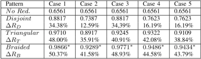
TABLE II: Comparison of the reliability provided by each pattern.
Pattern Case 1 Case 2 Case 3 Case 4 Case 5
N o Red. 0.6561 0.6561 0.6561 0.6561 0.6561 Disjoint 0.8817 0.7387 0.8817 0.7623 0.7623 ∆RD 34.38% 12.59% 34,39% 16.19% 16.19% T riangular 0.9710 0.8917 0.9245 0.9322 0.9109 ∆RT 48.00% 35.91% 40.91% 42.08% 38.84% Braided 0.9866∗ 0.9289∗ 0.9771∗ 0.9486∗ 0.9434∗ ∆RB 50.37% 41.58% 48.93% 44.58% 43.79%
Table II gives the reliability obtained in each case by each pattern as well as the relative increase in reliability with regard
to the No-Redundancy pattern. The character ’*’ denotes the best reliability achieved for the case considered.
Figure 7 depicts the reliability of an end-to-end transmission from S to D for the three pattern studied in the five cases considered. The Disjoint-path pattern provides an increase in reliability ranging from 34% for the case 1 to 12.59% for the cases 2 and 5. In any case, it is dominated by both the Triangular and the Braided patterns that provide the highest increase in reliability reaching 48% and 50% in case 1, respectively. The Braided pattern outperforms the Triangular pattern in all the cases studied, with a reliability that in the worst case (i.e. case 2, where any link that does not belong to the primary path has a lower reliability), is equal to 0.9289. In the best case (i.e. case 1 where all links have the same high reliability), it provides a reliability reaching 0.9866. The dominance of the Braided pattern from the reliability point of view is due to the two possibilities for an alternate parent to receive the message in a Braided pattern, instead of only one possibility for the Triangular pattern.
0.65 0.7 0.75 0.8 0.85 0.9 0.95 1
Case1 Case2 Case3 Case4 Case5
Reliablity
No Redundancy Disjoint Triangular Braided
Fig. 7: Reliability of an end-to-end transmission for each pattern in the 5 cases studied.
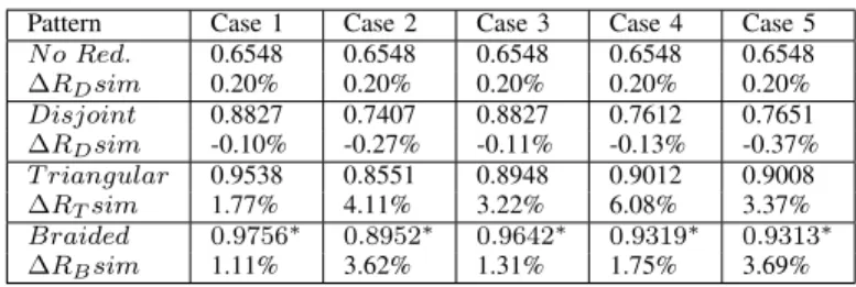
2) Simulation results for the reliability of each pattern: The theoretical results listed in Table II are now compared with simulation results obtained with NS3. Each simulation result is the average of 30 simulation runs. To generate unreliable links, a random generator is used per unreliable link: a message sent on this link is received with a probability equal to the link reliability. The source S generates 1000 messages and the destination delivers without duplication the messages received. Figure 8 depicts the reliability of an end-to-end transmission from S to D for the three pattern studied in the five cases considered. As expected, this figure is very similar to Figure 7 depicting the theoretical results obtained.
Table III gives the simulation results obtained by each pattern in the five cases studied. As expected, the simulation results are very close to the theoretical results. The relative difference given in the line ∆RXsim, is less than 0.20% for
the N oRedundancy configuration, 0.37% for the Disjoint pattern, less than 6.08% for the T riangular pattern and less than 3.69% for the Braided pattern. In any case, the Braided pattern is the most reliable.
0.6 0.65 0.7 0.75 0.8 0.85 0.9 0.95 1
Case1 Case2 Case3 Case4 Case5
Reliablity
No Redundancy Disjoint Triangular Braided
Fig. 8: Simulation results for the reliability of an end-to-end transmission for each pattern in the 5 cases studied.
TABLE III: Reliability of each pattern get by simulation.
Pattern Case 1 Case 2 Case 3 Case 4 Case 5
N o Red. 0.6548 0.6548 0.6548 0.6548 0.6548 ∆RDsim 0.20% 0.20% 0.20% 0.20% 0.20% Disjoint 0.8827 0.7407 0.8827 0.7612 0.7651 ∆RDsim -0.10% -0.27% -0.11% -0.13% -0.37% T riangular 0.9538 0.8551 0.8948 0.9012 0.9008 ∆RTsim 1.77% 4.11% 3.22% 6.08% 3.37% Braided 0.9756∗ 0.8952∗ 0.9642∗ 0.9319∗ 0.9313∗ ∆RBsim 1.11% 3.62% 1.31% 1.75% 3.69% B. Overhead
The increase in reliability is obtained at the cost of a higher overhead that we now want to evaluate. The two node-disjoint paths, the Triangular pattern and the Braided pattern, involve the same number of intermediate nodes: 2 ∗ (L − 1), where L is the length of the path between S and D. Hence the total number of nodes involved by each redundant pattern is:
N odes = 2 ∗ L.
We now compute the number of message transmissions generated as a function of the path length.
• Disjoint-path: Each node on the path, except the desti-nation, transmits the message. Since there are two paths, there are 2 ∗ L message transmissions.
T ransmissions = 2 ∗ L.
• Triangular: Each node on the primary path, except the destination and the nodes one-hop away from the des-tination, transmits the message to its default parent and to its alternate parent, leading to a total of 2 ∗ (L − 1) transmissions. The intermediate node on the primary path, one-hop away from the destination transmits the message only to the destination. In addition, each alternate parent transmits the message only to its triangular parent, lead-ing to L − 1 transmissions. Hence a total of:
T ransmissions = 3 ∗ L − 2.
• Braided: Each node on the primary path and on the alternate path, except the destination and the nodes
one-hop away from the destination, transmits the message to two parents, leading to a total of:
T ransmissions = 4 ∗ (L − 1).
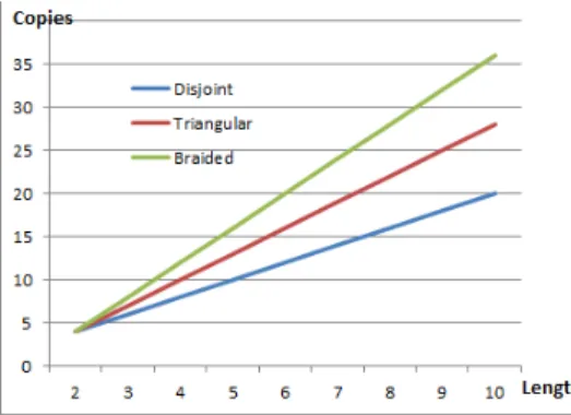
For instance, the total number of transmissions is for a redundancy pattern of length 4, 8 for the Disjoint-path pattern, 10 for the Triangular pattern and 12 for the Braided pattern, respectively. More generally, Figure 9 depicts the number of message transmissions generated by each pattern studied as a function of the length of the path.
Fig. 9: Number of message transmissions generated by each pattern as a function of path length.
C. Energy consumed by an end-to-end transmission
Since the TSCH schedule enables each node to know when it is allowed either to transmit its messages or to receive messages, each node enters the Sleep mode each time slot where it is not involved in a communication. The Sleep mode enables the node to save a considerable amount of energy and hence to considerably increase its energy autonomy. As a consequence, the energy consumed by a node involved in an end-to-end communication is consumed while transmitting or receiving a message or an acknowledgment. However, due to failure, a node may wait for a message that it will never receive in this slot. The energy consumed by each node during an end-to-end transmission is computed for the three patterns as follows. In any redundancy pattern, nodes S and D behave as follows:
- S transmits 2 messages and receives their acknowledgment. - D receives 2 messages and acknowledge them.
1) Disjoint-path pattern:
In the Disjoint-path pattern, each node, except S and D, behaves as follows:
- Ni receives one message, acknowledges it, forwards it and
receives its acknowledgment.
E(S) = 2 ∗ ET x(msg) + 2 ∗ ERx(ack)
E(Ni) = ERx(msg) + ET x(ack) + ET x(msg) + ERx(ack)
E(D) = 2 ∗ ERx(msg) + 2 ∗ ET x(ack)
The total energy ED consumed by an end-to-end
transmis-sion in a Disjoint-path pattern is given by:
ED= 2 ∗ L ∗ (ET x(msg) + ERx(ack) + ERx(msg) + ET x(ack)) (3)
2) Triangular pattern:
In the Triangular pattern, each node, except S and D, behaves as follows:
- Ni,han intermediate node on the primary path that is neither
a 1-hop neighbor of S nor a 1-hop neighbor of D, receives 2 messages, acknowledges them, forwards one message to its both parents and receives their acknowledgment. There are (L − 3) such nodes.
- Ni,a an alternate parent (i.e. N2, N4 and N6 in Figure 3)
receives one message, acknowledges it and forwards it to its triangular parent. There are L − 1 such nodes.
- Ni,S the one-hop neighbor of S on the primary path (i.e. N1
in Figure 3) receives one message, acknowledges it, forwards it to its both parents and receives their acknowledgments. - Ni,D the one-hop neighbor of D on the primary path (i.e.
N5 in Figure 3) receives 2 messages, acknowledges them,
forwards one message to D and receives its acknowledgment.
E(S) = 2 ∗ ET x(msg) + 2 ∗ ERx(ack)
E(Ni,h) = 2 ∗ ERx(msg) + 2 ∗ ET x(ack) + 2 ∗ ET x(msg)
+2 ∗ ERx(ack)
E(Ni,a) = ERx(msg) + ET x(ack) + ET x(msg) + ERx(ack)
E(Ni,S) = ERx(msg) + ET x(ack) + 2 ∗ ET x(msg) + 2 ∗ ERx(ack)
E(Ni,D) = 2 ∗ ERx(msg) + 2 ∗ ET x(ack) + ET x(msg) + ERx(ack)
E(D) = 2 ∗ ERx(msg) + 2 ∗ ET x(ack)
The total energy ET consumed by an end-to-end
transmis-sion in the Triangular pattern is given by:
ET= (3 ∗ L − 2) ∗ (ET x(msg) + ERx(ack) + ERx(msg) + ET x(ack)) .
(4)
3) Braided pattern:
In the Braided pattern, each node behaves as follows: - Ni,h an intermediate node that is neither a 1-hop neighbor
of S nor a 1-hop neighbor of D, receives 2 messages, acknowledges them, forwards one message to its both parents and receives their acknowledgment. There are 2 ∗ (L − 3) such nodes.
- Ni,S the two one-hop neighbors of S (i.e. N1 and N2 in
Figure 3) receive one message, acknowledge it, forward it to their both parents and receive the 2 acknowledgments. - Ni,D the two one-hop neighbors of D (i.e. N5 and N6 in
Figure 3) receive 2 messages, acknowledge them and forward one message to D and receive its acknowledgment.
E(S) = 2 ∗ ET x(msg) + 2 ∗ ERx(ack) E(Ni, h) = 2 ∗ ERx(msg) + 2 ∗ ET x(ack) + 2 ∗ ET x(msg) +2 ∗ ERx(ack)
E(Ni,S) = ERx(msg) + ET x(ack) + 2 ∗ ET x(msg)
+2 ∗ ERx(ack)
E(Ni,D) = 2 ∗ ERx(msg) + 2 ∗ ET x(ack) + ET x(msg)
+ERx(ack)
E(D) = 2 ∗ ERx(msg) + 2 ∗ ET x(ack)
The total energy EB consumed by an end-to-end
transmis-sion in the Braided pattern is given by:
EB= 4 ∗ (L − 1) ∗ (ET x(msg) + ERx(ack) + ERx(msg) + ET x(ack)) .
4) Comparison of the total energy required by each pattern: Equations 3, 4 and 5 show that the total energy consumed by an end-to-end transmission in each pattern studied is propor-tional to the number of transmissions performed by each pat-tern. The proportionality coefficient is equal to ET x(msg) +
ERx(ack) + ERx(msg) + ET x(ack). Hence, the curves
de-picting the total energy consumed by each pattern have the same shape as those giving the number of transmissions as a function of the path length illustrated in Figure 9.
D. Impact on the schedule and the delivery time
The management of the unreliability of wireless links and nodes has a strong impact on the schedule used: the schedule set up for a perfect wireless network where nodes and links are assumed to never fail, is not sufficient. In an unreliable network, additional slots must be allocated to enable the additional transmissions that may be either retransmission on the same link or transmission on another link. There are different approaches based on over-provisioning, which vary in the way to consider the wireless links and in the nature of the additional slots allocated.
Wireless links in the primary path may be considered: - either as a whole set. The reliability of the path is evaluated and a number of disjoint paths is computed to provide the requested reliability. This solution is simple but may lead to useless transmissions (e.g. on the most reliable links for instance).
- or independently. The number of copies of the message is computed at each hop. As a consequence, the number of copies is perfectly tuned to the reliability of the wireless link, but at the cost of some additional processing. In addition, if the link quality varies, a new computation is needed.
- or according to a mixed approach. Some links are considered individually, whereas others are considered as a group. A mixed approach tends to limit the complexity.
The additional slots allocated may be:
- dedicated: with each transmission is associated an additional slot to enable a retransmission on the same link or a transmission on another link, in case of failure. The sender and the receiver of each additional slot are perfectly identified and no other nodes are allowed to use this slot. The advantage is that these additional slots can be scheduled in an order that minimizes the end-to-end delivery time. The main drawback is the possible high number of allocated slots that may remain unused in case of successful transmissions, when a detection recovery approach is adopted. In case of a masking approach, this drawback does not exist, since the transmission is done systematically on both links.
- shared: To avoid the previous drawback, additional slots are allocated in shared mode, where several transmitters may use them. In such a case, a collision will occur and a CSMA/CA protocol ([9], [2]), specific to TSCH, is used between the competing transmitters. Shared cells tend to limit the number of additional cells needed, but at the cost of message losses
in case of collision.
- some dedicated cells and some other shared cells: this combination benefits from the advantages of both previous approaches only if all the transmitters scheduled in the same slot and channel do not cause a collision.
In this section, we call perf ect schedule the schedule in a perfect network (i.e. no redundancy is needed) and redundant schedule the schedule where a redundancy pattern is used. We adopt the following additional assumptions:
• A7 In the perf ect schedule, each node has at least as
many opportunities to transmit as messages to transmit to the destination, including those that it has to forward.
• A8 In the perf ect schedule, any message transmitted in
a Slotframe is delivered to the destination in the same Slotframe, assuming no failure.
• A9 Only for the evaluation of the delivery time (i.e. in
this section), we assume that only dedicated cells are used to schedule additional transmissions.
The perfect schedule of the end-to-end transmission from S to D is given by Table IV, where a line corresponds to a channel offset and a column to a timeslot. For instance, in the timeslot of offset 3 from the beginning of the Slotframe and in the channel corresponding to the offset 0, node N5will
transmit its message to node D.
TABLE IV: Perfect schedule of the end-to end transmission.
0 1 2 3
0 S → N1 N1→ N3 N3→ N5 N5→ D
In an unreliable network, all the transmissions generated by each redundancy pattern should be scheduled by the scheduler. Since the end-to-end transmission from S to D requires L transmissions in a perfect network, the scheduler has to schedule:
• L additional transmissions for the Disjoint-path pattern. • 2 ∗ (L − 1) additional transmissions for the Triangular
pattern.
• 3 ∗ L − 4 additional transmissions for the Braided pattern.
The possibility of scheduling these additional transmissions in the slots already used by the perf ect schedule strongly depend on the interferences generated by these transmissions and by those belonging to the perf ect schedule. The interferences depend on the network topology, where additional wireless links may exist, even if they are not used in the routing tree. These additional links may cause conflicts that should be avoided by the scheduler. Nevertheless, the larger the number of additional transmissions, the larger the probability of using additional slots.
1) Disjoint-path pattern:
Property 1: The schedule of the Disjoint-path pattern re-quires 1 + δminterf slots more than the perf ect schedule,
where δminterf = 0 if the destination has multiple wireless
P roof : The source is unable to simultaneously transmit its message to its both parents (i.e. neither in the same dedicated cell, nor in the same slot but on two different channels). Hence, the two transmissions are serialized. After the transmission of the source on each path, two nodes belonging to the same rank transmit in the same slot: at each slot, the message progresses toward the destination on both paths. In addition, since on each path any intermediate node forwards the message it has received, the schedule should reflect this order. If the destination has multiple wireless interfaces, it may receive two transmissions in the same slot but on different channels. Hence the property.
Table V gives the schedule of end-to-end transmission accord-ing to the Disjoint-pattern. Five slots are needed, one more than the perfect case.
TABLE V: Schedule of the end-to end transmission according to the Disjoint-path pattern.
0 1 2 3 4
0 S → N1 S → N2 N1→ N3 N3→ N5 N5→ D
1 N2→ N4 N4→ N6 N6→ D
2) Triangular pattern:
Property 2: The number of additional slots required by the Triangular pattern is equal to L − 1 + δminterf, where
δminterf = 0 if the destination has multiple wireless
inter-faces, and 1 otherwise.
P roof : As previously, the two transmissions of the source are serialized. After the transmission of the source on each path, a primary intermediate node transmits to its alternate parent while its sibling node (i.e. alternate parent at the same rank as itself) transmits to its triangular parent in the same slot. In other words, the two transmissions corresponding to the two branches of the ’X’ in the Triangular pattern are scheduled in the same slot (e.g. N1 → N4 and N2 → N3 in Figure 3). If
the destination has multiple wireless interfaces, it may receive two transmissions in the same slot but on different channels. Hence the property.
Table VI gives the schedule of end-to-end transmission accord-ing to the Disjoint-pattern. Seven slots are needed, L − 1 = 4 more than in the perfect case.
TABLE VI: Schedule of the end-to end transmission according to the Triangular pattern.
0 1 2 3 4 0 S → N1 S → N2 N1→ N3 N1→ N4 N3→ N5 1 N2→ N3 5 6 0 N3→ N6 N5→ D 1 N4→ N5 N6→ D 3) Braided pattern:
Property 3:The number of additional slots required by the Braided pattern is equal to L−1+δminterf, where δminterf =
0 if the destination has multiple wireless interfaces, and 1 otherwise. This is the same number as the Triangular pattern. P roof : In addition to the parallelism of the transmissions done by the two branches of the ’X’ appearing in the Braided pattern, the vertical transmissions are also parallelized (see
for instance the transmissions N1 → N3 and N2 → N4 in
Figure 4. Hence the property.
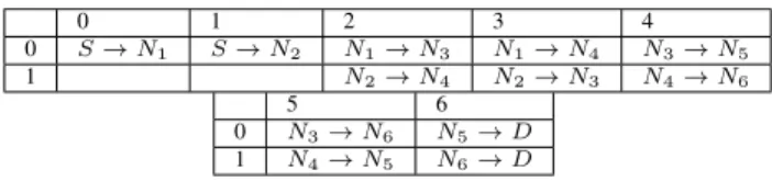
Table VII gives the schedule of end-to-end transmission according to the Disjoint-pattern. Seven slots are needed, L − 1 = 4 more than the perfect case.
TABLE VII: Schedule of the end-to end transmission accord-ing to the Braided pattern.
0 1 2 3 4 0 S → N1 S → N2 N1→ N3 N1→ N4 N3→ N5 1 N2→ N4 N2→ N3 N4→ N6 5 6 0 N3→ N6 N5→ D 1 N4→ N5 N6→ D
4) Upper bound on the delivery time:
We now provide an upper bound on the delivery time of the message to its destination.
Property 4: An upper bound on the delivery time of an end-to-end transmission, where the last transmission scheduled occupies the slot offset LastSlotU sed, is given by:
T Deliv ≤ Sf rameSize + (LastSlotU sed + 1) ∗ SSize (6) where LastSlotU sed is the offset of the last slot where a transmission is scheduled, Sf rameSize and SSize denote the size in ms of the Slotframe and the Slot, respectively. P roof : It corresponds to the worst case where a message is generated when the last slot granted to the node considered is just finishing, the node has to wait for the next Slotframe to transmit this message. According to A8, it will be delivered
to the destination in the same Slotframe. Hence the equation. E. Discussion
We are now able to make some recommendations about the choice of a redundancy pattern for a given application profile supported by a given network topology. For a given industrial application with its own reliability, latency and node power autonomy constraints, the choice of the redundancy pattern strongly depends on the reliability of the links composing the TSCH network. If the No Redundancy pattern applied to this network topology provides a reliability that meets the application constraint, it is chosen.
Otherwise, a redundancy pattern should be chosen. Since the increase in reliability is obtained at the cost of a higher over-head that decreases the power autonomy of wireless nodes, the smallest redundancy degree providing the requested reliability should be chosen: the Disjoint-path pattern with an overhead proportional to 2 ∗ L, the Triangular pattern with an overhead proportional to 3 ∗ L − 2 and finally the Braided pattern with an overhead proportional to 4 ∗ (L − 1). Notice that even if the network topology provides all the links used by the Braided pattern, sometimes it is better to select the Triangular pattern that does not use the vertical links between the alternate parents to preserve the autonomy of wireless nodes.
In addition, if the latency constraint is strong, there is no other choice than a masking strategy where the response time does not depend on the occurrence of an error. Otherwise, if a detection/recovery strategy meets the latency constraint and
the node power autonomy constraint is high, this strategy will be preferred. It would allow to save energy because the error recovery is done only when an error has occurred.
VI. CONCLUSION
In this paper, we have presented three redundancy patterns, namely the Disjoint-path, the Triangular and the Braided pat-terns, improving the reliability of an end-to-end transmission in a TSCH network, a potential candidate for the IoT used by the Industry 4.0. A detailed analysis of the performances that matter for Industry 4.0 is done. The reliability provided by each pattern, the delivery time and the overhead in terms of the number of transmissions generated by each pattern as well as the amount of energy consumed by an end-to-end transmission allows us to conclude that the Braided pattern provides the highest reliability but with an overhead approximately twice the overhead of the Disjoint-path pattern and 4/3 the over-head of the Triangular pattern. These performance results are corroborated by simulations performed with NS3 for various configurations.
ACKNOWLEDGMENT
Study co-funded by CNES and Inria in the framework of the CNES Launchers Research and Technology program.
REFERENCES
[1] C. Adjih, T. Clausen, P. Jacquet, A. Laouiti, P. Minet, P. Muhlethaler,
A. Qayyum, and L. Viennot. RPL: Optimzed Link State Routing
Protocol (OLSR). RFC 3626, RFC Editor, October 2003.
[2] S. Chen, T. Sun, J. Yuan, X. Geng, C. Li, S. Ullah, and M. Abdullah Alnuem. Performance Analysis of IEEE 802.15.4e Time Slotted Channel
Hopping for Low-Rate Wireless Networks. KSII Transactions on
Internet and Information Systems, 7(1):1–21, 2013.
[3] D. De Guglielmo and G. Anastasi and A. Seghetti. Advances onto the Internet of Things, chapter From IEEE 802.15.4 to IEEE 802.15.4e: A Step Towards the Internet of Things. Springer, 2014.
[4] D. De Guglielmo, S. Brienza, and G. Anastasi. IEEE 802.15.4e: A survey. Computer Communication 2016, 88:1–24, 2016.
[5] G. Fairhurst and L. Wood. Advice to link designers on link Automatic Repeat reQuest (ARQ). RFC 3366, IETF, August 2002.
[6] G. Z. Papadopoulos and T. Matsui and P. Thubert and G. Texier and T. Watteyne and N. Montavont. Leapfrog Collaboration: toward determinism and predictability in industrial IoT applications. In IEEE Intern. Conference on Communications, ICC, Paris, France, May 2017. [7] H. Kurunathan and R. Severino and A. Koubaa and E. Tovar. Towards Worst-Case Bounds Analysis of the IEEE 802.15.4e. In RTAS 2016, 22nd IEEE Real-Time and Embedded Technology and Applications Symposium, Vienna, Austria, 2016.
[8] M. Hermann, T. Pentek, and B. Otto. Design principles for industrie 4.0 scenarios. In Proceedings of the 2016 49th Hawaii International Conference on System Sciences (HICSS), HICSS ’16, pages 3928–3937, Washington, DC, USA, 2016. IEEE Computer Society.
[9] IEEE SA. IEEE Standard for Local and metropolitan area networks– Part 15.4: Low-Rate Wireless Personal Area Networks (LR-WPANs) – Amendment 1: MAC sublayer. IEEE Std 802.15.4e-2012 (Amendment to IEEE Std 802.15.4-2011), IEEE, February 2012.
[10] J.Edmonds and R.M. Karp. Theoretical improvements in algorithmic efficiency for network flow problems. Journal of the ACM. Association for Computing Machinery, 19(2):248–264, 1972.
[11] H. Kagermann, W. Wahlster, and J. Helbig. Recommendations for
implementing the strategic initiative Industrie 4.0: Final report of the
Industrie 4.0 working group. Technical report, Frankfurt, Germany,
2013.
[12] A. Laouiti, P. Jacquet, P. Minet, L. Viennot, T. Clausen, and C. Adjih. Multicast Optimized Link State Routing. Inria Research Report RR4721, Inria, Feb 2003.
[13] S. Rathinavel and V. Pandi and A. Sivaraman. On the exploration of adaptive mechanisms providing reliability in clustered WSNs for power plant monitoring. Scientific World Journal, 2016, 2016.
[14] T. Watteyne and J. Weiss and L. Doherty and J. Simon. Industrial
IEEE802.15.4e Networks: performance and trade-offs. In IEEE ICC 2015 SAC Internet of Things, London, UK, June 2015.
[15] T. Winter, P. Thubert, A. Brandt, J. Hui, R. Kelsey, P. Levis, K. Pister, R. Struik, JP. Vasseur, and R. Alexander. RPL: IPv6 Routing Protocol for Low-Power and Lossy Networks. RFC 6550, RFC Editor, March 2012.
[16] X. Vilajosana and Q. Wang and F. Chraim and T. Watteyne and T. Chang and K. Pister. A Realistic Energy Consumption Model for TSCH Networks. IEEE Sensors Journal, 14(2), February 2009.