EFFECT OF BORROWING CONSTRAINTS ON LOCATION CHOICE: EVIDENCE FROM THE PARIS REGION

HAL Id: hal-01294215

https://hal.archives-ouvertes.fr/hal-01294215

Preprint submitted on 28 Mar 2016

HAL is a multi-disciplinary open access

archive for the deposit and dissemination of sci-entific research documents, whether they are pub-lished or not. The documents may come from teaching and research institutions in France or

L’archive ouverte pluridisciplinaire HAL, est destinée au dépôt et à la diffusion de documents scientifiques de niveau recherche, publiés ou non, émanant des établissements d’enseignement et de recherche français ou étrangers, des laboratoires

EFFECT OF BORROWING CONSTRAINTS ON

LOCATION CHOICE: EVIDENCE FROM THE PARIS

REGION

Sophie Dantan, Nathalie Picard

To cite this version:

Sophie Dantan, Nathalie Picard. EFFECT OF BORROWING CONSTRAINTS ON LOCATION CHOICE: EVIDENCE FROM THE PARIS REGION. 2016. �hal-01294215�

EFFECT OF BORROWING CONSTRAINTS ON LOCATION CHOICE: EVIDENCE FROM THE PARIS REGION

Sophie Dantan1 _{and Nathalie Picard}2 March 2016

ABSTRACT

This paper investigates the determinants of residential segregation in Paris region by disentangling households’ preferences for local amenities, for dwelling type and for homeownership, in a nested logit model. This model is extended to account for unobservable borrowing constraints which might prevent some households from purchasing a dwelling. A counterfactual distribution of socio-demographic characteristics across the Paris region is then built by relaxing those constraints. The comparison of the actual and counterfactual distributions suggests that if their credit constraints were alleviated, households would tend to locate further from Paris. In particular if constraints were relaxed only on the poorest households, they would not be likely to mix with the richest households.

JEL classification codes : R21, R23, R31

Key words: Homeownership, Tenure choice, Borrowing constraints, Residential segregation, Suburbanization, Urban sprawl, Location choice model, Endogenous choice sets.

1. Introducti on

Various housing policy measures are implemented to favor the access of poor households to homeownership, in France as in other countries. Measures such as the deductibility of mortgage interests have been rapidly abandoned, while other measures such as the provision of zero-interest-rate loans have been implemented under various forms and restrictions. One of the motives for implementing such measures is to enhance social mobility by enabling the poorest households to cumulate and transmit housing assets.

Little attention has been paid to the effect of such a homeownership-enhancing policy on residential segregation, which is however an important determinant of social mobility (Combes et al. 2008, Causa et al. 2010, Gobillon et al. 2011). In particular, if relaxing constraint on ownership for poor households reinforces residential segregation, the expected positive effect on social mobility might be significantly reduced. Measuring to what extent residential segregation is exacerbated or attenuated by liquidity constraints contributes to determine the relevance of enhancing homeownership for increasing social mobility. The ambiguity comes from the fact that households who are eligible to these measures may prefer buying in the poor suburbs rather than renting in the rich Central part of the city.

We highlight this issue by evaluating the importance of housing liquidity constraints in explaining the social sorting in the Paris region. To do so, we model household preferences for housing characteristics and for tenure status (ownership vs. tenancy) and then extend our model to account for the effect of liquidity constraints on location demand.

The effect of liquidity constraints on segregation is then evaluated by comparing the distribution of households with and without liquidity constraints. In this purely normative exercise, prices and socio-demographic composition are being held constant. The objective of this normative evaluation of policy measures is indeed to evaluate what each household

for other households. By contrast, a descriptive and predictive analysis of policy measures would require computing their aggregate effects on the endogenous equilibrium of the housing market, that is, changes in socio-demographic composition, in housing prices, and plausible assumptions on real estate supply reactions to changes in demand. Such a predictive analysis is out of the scope of this article.

2. Locati on choi ce and tenure status

In the economic literature, the choices of tenure status and of housing consumption have long been studied separately: the former by assuming that tenure choice results from the comparison of the respective costs of owning and renting (Smith et al. 1988 for a review), the latter by assuming that tenure status is exogenous and maximizes the utility derived from housing consumption (for instance Artle and Varaiya, 1978). However, as underlined by Lee and Trost (1978), Rosen (1979), and King (1980), housing consumption and tenure choice both result from the same utility maximization process, which implies that they are determined by common variables.

2.1. Tenure choice and life cycle: household decisions and market imperfections Household decision whether to rent or own a dwelling is the result of a complex mechanism since the acquisition of a dwelling responds to dual motives, namely housing investment and housing consumption.

Households who invest in the ownership of a dwelling often have to engage in a long-term mortgage and then to adapt their consumption path. As a consequence, life-cycle effects might also play an important role in tenure status choice. According to Artle and Varaiya (1978), households tenure choice results from the maximization of their life-cycle consumption of non-housing good. The most patient households should then theoretically

improve their dwelling) at the middle and liquidate their housing equity asset by selling their home and renting another one at the end of their life-cycle3_{. By contrast, the most impatient}

households should favor their current consumption and choose permanent tenancy. Bequest motives or altruism toward their descendants can however attenuate the transition from ownership to renting among the elderly (Megbolugbe et al 1997, de Palma et al 2015). To account for the fact that housing is also a consumption good, Henderson and Ioannides (1983) develop a two-period model combining housing demand for consumption purpose, on one hand, and housing demand for investment purpose, on the other hand. Both demands are determined under a common budget constraint, which is similar for owners and renters (owner-occupiers rent to themselves). Under some specific conditions, they show that the propensity to own-occupy a dwelling (rather than renting it) is higher among individuals who are impatient or expect a decrease in their income. They also show that wealth increases the likelihood to purchase one’s dwelling only if the income elasticity of housing investment exceeds that of housing consumption.

Liquidity constraints, transaction cost and distortive tax modify the return to housing investment and can make it less competitive compared to the return of savings. Consequently, the budget constraint might differ between owner-occupiers and renters when financial markets are imperfect. For instance, the tax on rental income paid by landlords but not by owner-occupiers makes the ownership of a dwelling to rent out less profitable. On the opposite, the deductibility of paid mortgage interest and the zero-mortgage-interest loan make the housing investment more attractive. Similarly, a lower mortgage interest rate or a higher borrowable amount proposed to the wealthiest households might increase their housing investment and help explaining why they are more likely to purchase their home than the poorest households.

Liquidity constraint might influence residential segregation in two ways: it might influence both household decision to move and household location choice when moving. Concerning the mobility decision, Gobillon and Le Blanc (2004, 2008) develop a 2-period tenure choice model with an individual-specific borrowable amount and apply it to the case of the French zero-interest loan PTZ (Prêt à Taux Zéro). They show that this policy measure has increased ownership among poor households who would have stayed in their previous (rented) dwelling otherwise. However, it mainly benefits households which would anyway have moved and purchased a dwelling even without the PTZ.

We extend their approach and results by modelling the effects of liquidity constraints on household simultaneous choices of tenure and location, in the case of the Paris Region.

2.2. Residential segregation

Residential segregation in Paris region mainly consists in the concentration of the richest households inside Paris and close Western suburbs, while the poorest households tend to live in Northern and Eastern suburbs. Such a phenomenon is consistent with a monocentric model in which household income has a stronger positive effect on the valuation of accessibility of the Central Business District (CBD, here Paris intra muros) than on its demand for dwelling size (Alonso 1964, Mills 1967, Muth 1969, Wheaton 1977). Residential segregation can also be explained by a Tiebout-like (1956) mechanism which leads the richest households to concentrate in the CBD and then to induce an increase in housing prices which excludes poor households from the CBD (Bénabou 1995). In this latter case, social sorting is likely to be exacerbated by financial market imperfections which might prevent poor families from borrowing to acquire their preferred dwelling size and preferred location. Brueckner, Thisse and Zénou (1999) develop an alternative model in which the location choice depends not only on housing price and commuting cost but also on the level of amenities, assumed exogenous

increases with income (more rapidly than housing consumption). They show that if the CBD has a great advantage in the provision of amenities, then rich households are likely to concentrate in the center and poor households in the suburbs. By contrast, if the level of amenities slightly decreases or even increases with the distance to the CBD, the reversal might occur. This result explains why the concentration of rich households in the CBD is exacerbated when the CBD concentrates amenities (like in Paris) and is reversed when there are more amenities in suburbs (like in Detroit). They also show that even in the case where the level of some endogenous “modern” amenities increases with the local average income level, the concentration of rich households in the center is the only possible equilibrium when the exogenous amenity advantage of the center is large enough (as may be the case of Paris, for historical reasons).

As suggested above, another potential explanation for residential segregation might rely on household unequal access to ownership. However, the models of residential segregation mentioned above neglect tenure choice decisions. As a consequence, such models cannot be used to evaluate the effect of barriers to ownership on residential segregation. In Sections 3.1 to 3.2, we propose an alternative explanation of residential segregation, which accounts simultaneously for the effect of tenure status and liquidity constraint on location choice and, thus, on residential segregation.

Few empirical models relate housing demand and tenure choice (Elder and Zumpano 1991; Rappaport 1996) and none of them explicitly considers the effect of market imperfections on tenure choice. By contrast, Henderson and Ioannides (1986) evaluate this effect by estimating simultaneously the parameters of the probability to be constrained to rent and the probability to prefer ownership (by maximizing a joint likelihood function). However, they disregard residential location choice. In Sections 3.3 and 3.4, we present an estimation strategy which fills the gap between these approaches. The econometric model developed and estimated is

particularly useful to evaluate the effect of liquidity constraints on location choice and then on residential segregation.

3. M odel speci ficati on

3.1. Structural monocentric model

In this section, we develop a three-step monocentric model in which households choose their tenure status (s) in the first step, their distance (d) to the CBD and their level of local amenities (z) in the second step, and then their consumption of housing (H) and other goods (C) in the third step. The only source of heterogeneity between households considered in this section is income. Our model mainly builds upon the amenity-based location model developed by Brueckner et al. (1999), especially concerning endogenous equilibrium prices. Rather than analysing the determinants of equilibrium prices, we borrow their assumptions and conclusions concerning endogenous prices, in order to focus on household decisions conditional on prices, and to generalize their results in terms of household behaviour and heterogeneity.

Consistently with Section 2, our model introduces the distinction between owners and renters. The model is first extended to introduce a potential liquidity constraint, consistently with Section 2.1. It is then further extended to a more realistic discrete choice model in which household preferences are heterogeneous and distance d to CDB and local amenities z are determined by the discrete location j. Finally, the model is further extended by considering also dwelling type (T, either flat or house) in the first step of the program (at the same time as tenure status S). Prices then also depend on dwelling type T.

Definition D1)

Household i is characterized by income y_i , bounded by a finite value max _i i

space H and on consumption C of a composite good, which price is normalized to 1. Local amenities z are valued by an increasing and concave function (z), defined over  and further specified in Assumption H1). The distance d to the CBD is not valued directly, but only indirectly, through a commuting cost function specified in Assumption H4) and through dwelling price



S(d,z), specified in Assumption H2).

Assumption H1)

The function (z) is continuous and twice derivable on  and such that: '(z)>0 z;

''(z)<0 z; lim

 

and lim

 

z z   z z    .

The price of a dwelling



S(d,z), further specified in Assumption H2), equals its expected use cost when bought (S = “own”) and its rental price when rented (S= “rent”).

In contrast with the models analysed in Bruecker-Thisse-Zenou, the distance d and amount of amenities z are assumed here to entail some degree of independent variation, so that it makes sense to consider partial derivatives with respect to d and to z. Such a hypothesis is consistent with the observation that, at the same distance of Paris, the level of amenities and the concentration of rich households tend to be higher in Westerm suburbs than in Eastern suburbs.

Assumption H2)

The function



S(d,z) is continuous and twice derivable on + and such that:





_

_





_

_





















 

 

0 1 2 , , 0 , ; 0 , ;

lim , ; lim , 0; lim , 0; lim , ,

, . S S S S S S S d d z z S S S d z d z d z d z d z d z d z d z d z d z d z                                     

Assumption H2) is consistent with the finding by Brueckner-Thisse-Zenou (1999) that price must decrease with distance to ensure that utility is uniformly-distributed.

The price elasticity to distance d and to amenities z are denoted, respectively, by

 

_{   }

   

_{ }

 

 

   

_{   }

_{ }

 

0 ) , ( 1 ) , ( and 0 ) , ( 1 ) , ( 2 ' 2 2 1 ' 2 1 1 ' 1 2 1 2 ' 1               z z z d z d z d z z d z d d z d z d z d d z d d S S S S S S S S S z S S S S S S S S S d                   (1)

The multiplicative separability assumed in Assumption H2) ensures that the elasticity of price to distance d does not depend on amenities z, and vice-versa. We further assume increasing price elasticities: Assumption H3)

 

0 '  d S d  and _zS'

 

z 0.

Household i also incurs an increasing commuting cost t(d), defined over + _{and specified in}

Assumption H4). Assumption H4)

In Bruecker-Thisse-Zenou4 _{(1999) the commuting cost is a linear function of the distance}

(t''(d)=0), which is a special case here.

To fix ideas and to obtain closed-form solutions, we consider a specific (Cobb-Douglas) form for household utility as a function of consumption C and floor space H, as specified in Assumption H5).

Assumption H5)



C H z S



 

z



C





H



U , ; ; S (1S).S.ln  1S .ln , 0<S<1 and 0<S<1. (2) The parameter S measures the preference for consumption C over floor space H, whereas the parameter S measures the preference for amenities z over consumption bundle (C,H).

Most of the results obtained here would still hold if Utility were only assumed additively separable, increasing in amenities z and increasing and concave in consumption C and floor space H, with Inada conditions (infinite marginal utilities at zero consumption levels).

We consider a time period long enough to neglect saving and borrowing in the (inter-temporal) budget constraint:

) ( ) , (d z H t d C yi  



S   . (3)

Under Assumptions H1) to H5), we first show that the city has finite dimension. Different assumptions for limit conditions in H1) and H2) or in Definition D1) could lead to an infinite-dimension city without altering the other conclusions of the model.

Lemma 1

Household i can only select a distance d such that t(d)<yi. The size of the city is finite: there

exists a maximal finite distance D>0 and a finite maximal commuting cost T>0 such that t : [0;D]  [0;T] is a one-to-one mapping; its inverse, denoted by t-1_{(.) is continuous and}

increasing on [0;T].

Proof: See Appendix 8.1. ∎

The model is solved backwards, in three steps.

 In the third step of the program, household i maximizes its utility (2) subject to budget constraint (3), given household income yi, tenure status S, distance d (such that

t(d)<yi), and local amenities z, by choosing the optimal levels of housing good

) ; ; , ( * i y S z d

H and of other goods C*(d,z;S;y_i). This results in the indirect utility of household i with income yi conditional on tenure status S, on distance d and on

amenities z: U*(d,z;S;y_i)U



C*



d,z;S;y_i

 

,H* d,z;S;y_i



;z;S



. Lemma 2

Consider y_i

 

0,Y d, _0;t1

 

y_i _,z and S



own rent,



. Maximizing utility (2) under budget constraint (3) leads to optimal consumption levels C*



d,z;S;y_i



S



y_it

 

d



and









_{ }

 

z d d t y y S z d H S i_S i , 1 ; ; , *     

 , and to the indirect utility

 

z







y t

 

d









 

d z k y S z d U*( , ; ; _i) S S  1S ln _i   1S .1S .lnS , , (4)

where kS is a non-linear combination of the coefficients S and S.

 The second step of the program consists in choosing the distance d to CBD and the amount of local amenities z so as to maximize the indirect utility U*(d,z;S;yi) conditional on tenure status S and on income yi.

Under assumptions H1) to H5), the optimal distance and amount of local amenities resulting from the second step of the program are shown to be unique (see proofs of Lemmas 3 and 4 in Appendix 8.1) and are denoted by d*



S;y_i



and z*

 

S . Note that, under Assumption H5)5_,

the optimal distance depends on income, whereas the optimal level of amenities does not. Lemma 3

Under Assumptions H1) to H5), for any tenure status S, income yi and level of amenities z, the

indirect utility U*(d,z;S;yi) is a concave function of d on [0; t

-1_(y

i)[ and there exists a unique

optimal distance d*



S;yi





0;t 1(yi)





 which maximizes U*(d,z;S;yi).

Proof: See Appendix 8.1. ∎

Optimal location results from a trade-off between the price, which decreases when moving farther away from the CBD and the transportation cost, which increases when moving farther away from the CBD. Assumption H3) ensures that price decreases faster closer to CDB, whereas Assumption H4) ensures that transportation cost increase faster when farther away from the CBD.

Lemma 4

Under Assumptions H1) to H5), for any tenure status S, income yi and distance d  ]0; t-1(yi)[,

the indirect utility U*(d,z;S;yi) is a concave function of z on  and there exists a unique

optimal level of amenities z*

 

S  which maximizes U*(d,z;S;y_i).

Proof: See Appendix 8.1. ∎

The second step of the program results in the “further-indirect” utility U**_{(.) of household i}

with income yi conditional on tenure status S:



;

  

, ; ; ) ( ) ; ( * * * * * i i i U d S y z S S y y S U  . (5)

 The first step of the program simply consists in choosing, among the two possible tenures, the one which gives the highest “further-indirect” utility: household i buys a dwelling if and only if (iff) U**(own;yi)U**(rent;yi) and it rents a dwelling iff

) ; ( ) ; ( ** * * i i U rent y y own U  .6

3.2. Introduction of a liquidity constraint

The program developed in Section 3.1 neglects the liquidity constraints which, consistently with Section 2, may affect some households if they want to buy a dwelling during the first stage of their life cycle. To formalize the role of such constraints, we introduce in the model of Section 3.1 an upper limit max

i

A on the amount which can be spent on buying a household. According to Lemma 2, without such constraint, the optimal amount spent on buying a dwelling would be

 

d z H



d z S y









yi t

 

d



own i S       , * , ; ; 1 .

Such potential constraints do not affect the utility of renting a dwelling and thus does not modify the tenure choice of a household which prefers renting to buying (i.e.

) ; ( ) ; ( ** * * i i U rent y y own

U  in the model analysed in Section 3.1). By contrast, if household i

prefers buying (U**(own;yi)U**(rent;yi)), three situations may occur, as illustrated on Figure 1 and shown below. In this example, household i prefers ownership to tenancy if unconstrained and its optimal renting location is closer to the CBD (distance





1*

*

;y_i dR rent

d  ) than its optimal buying location ( *





1* 1*

; O R

i

d own y d d ).

i) If the potential constraint is not binding, the tenure choice is the same as in the model without constraint (upper right-hand side curve maximized at dO1* such that







 

1*



max

1own  y_i t dO A_i ).

ii) If the potential constraint is binding and moderate (A₂



1own







y_it

 

dO1*



on the intermediate right-hand side curve), household i is actually constrained and buys a cheaper dwelling, located farther away from the CBD: the constrained owning utility U~*(d,z*



own



;own;y_i,A₂) is maximized at dO2*>dO1* such that







 



2 * 2 1 y t dO A i own     and O





_i



_i



y rent U A y own own z d U~*( 2*, * ; ; , ₂) ** , . iii) If the potential constraint is binding and strong (A3 very small), household i is

actually constrained and prefers renting than buying its dwelling: the constrained owning utility U~*(d,z*



own



;own;y_i,A₃) is maximized at dO3*>dO1* such that







 



3 * 3

1own  y_it dO  A and_U~ _(dO _,z



_own



_{;own;yi,A) U}**



_rent,yi



3

* * 3

*  _.

Liquidity constraints have no effect on residential segregation in case i); they exacerbate segregation in case ii) and they reduce segregation in case iii). The aggregate effect of liquidity constraints on residential segregation thus depends on the correlation between

Figure 1: Illustration of the effect of credit constraint on tenure choice and optimal distance

The third step of the program is unchanged for S=rent. By contrast, when S=own, household i maximizes its utility according to:





 





, max , ; ; (1 ). .ln 1 .ln subject to ( , ) ( ) and . ( , )

own own own own

C H own i i own MaxU C H z own z C H y C d z H t d A H d z              _   _      . (6)

The constraint is binding iff the optimal expense on housing is larger than max

i

A , that is iff:







y t

 

d



A_imax  1own  _i . (7)

Lemma 5

If the maximum borrowable amount A_imax is larger than



own



_i

y  

1 , then the potential constraint is never binding. IfA_imax  



1 own



y_i, then there exists a unique threshold distance



y A



t y Ai _own

 

D i i i 0; 1 , max 1 max *              

 such that liquidity constraint is binding iff





*



max



* , ;yi yi Ai own d  .

The threshold *



yi,Aimax



is increasing in the income level y and decreasing in the i borrowable amount max

i

A ; it verifies0*



y_i,A_imax



t1

 

y_i .

Proof: If max





1 own

i i

A   y , then the optimal dwelling expense



  







 







max * 1 1 , ; ; ,z S y_i S d z S y_i t d S y_i A_i d H



 



   



  , so the potential

constraint is not binding. Assume now that max





1 own

i i

A   y . Then, given that own<1 and using Lemma 1, Eq. (7) can be rewritten:

 

y D t A y t i _{own i} i             1 max 1 1 0  , (8)

so there is a unique threshold distance



y A



t y Ai _own

 

D i i i 0, 1 , max 1 max *              

 such that the

optimal expense at *



y_i,A_imax



is : H*



*



y_i,A_imax



,z;S;y_i



S



*



y_i,A_imax



,z



 A_imax, and the constraint is binding iff d*



own;y_i



*



y_i,A_imax



.

Using Lemma 1 (t-1(.) is increasing), *



yi,Aimax



is increasing in income yi and decreasing in the borrowable amount max

i

A .∎

If the constraint is not binding, then the indirect utility is again given by Eq. (3) (for S = “own”). By contrast, when the constraint is binding, the chosen housing expense equals max

i

A ,

the optimal quantities are

 

d z A A own z d H _owni i , ) ; ; , ( ~* max max   and

 

d t A y A y own d

C~*( ; ; _i, _imax) _i  _imax  and the program results in the indirect utility of household i with income yi conditional on distance d, on local amenities z and on

 



 



max max max * ln ) 1 ( ) 1 ( ) , ( ln ) 1 ( ) 1 ( ln ) 1 ( ) , ; ; , ( ~ i own own own own own i i own own own i i A z d A d t y z A y own z d U                            . (9)

To sum up, under liquidity constraints, the indirect utility U of household i with income y~* i

and maximum borrowable amount max

i

A conditional on distance d, on local amenities z and on homeownership is:

 







max



* * max * max max max * , if ) ; ; , ( , if ) , , , ), ( ( ) , ; ; , ( ~ i i i i i own i i i i i A y d y own z d U A y d own z z d A d t A y U A y own z d U          . (10) Proposition 1:

The (owning) utility of Household i is not affected by liquidity constraints in locations which are far enough from the CBD, that is, if *



max



, i i d   y A . By contrast, if *



max



, i i d   y A ,

then liquidity constraints induce a loss of utility equal to

) , ; ; , ( ~ ) ; ; , ( * max * i i i U d z own y A y own z d

U  , which is a positive and decreasing function of d.

See proof in Appendix 8.2. ∎

Under binding liquidity constraint, the second step of the program is the same as in Section 3.1 except that U*(d,z;own;y_i) is now replaced byU~*(d,z;own;y_i,A_imax). The optimal

distance and quantity of local amenities, now denoted by d~*



own;y_i,A_imax



and

 

own z

 

own

z* *

~ _{ maximize the indirect constrained utility} ~*_{( , ; ; ,} max₎

i i A y own z d U

conditional on owning, on income yi and on maximal amountA_imax. These values are unique

(see proof of Proposition 1 in Appendix 8.2). The resulting “further-indirect” constrained utility of household i with income yi conditional on tenure status S is:



;



,~

 

; ; , ) ~ ( ~ ) , ; (

~** max * * max * max

i i i

i i

i A U d own y A z own own y A

y own

Obviously, for constrained households, U~**(own;y_i,A_imax)U**(own;y_i)). The proof of this result can easily be derived from Proposition 1. The utility



;



,~

 

; ; , ) ~ ( ~* * max * max i i i iA z own own y A y own d

U is lower than the utility U*(d~*



own;y_i

  

,z~* own;own;y_i) which is itself lower than U*(d*



own;y_i

  

,z* own;own;y_i) since d*



own;y_i



and z*own

maximize the indirect utility *(.,.; , ) i y own

U .

Proposition 2: When the optimal distance to the CBD without liquidity constraints is larger than the threshold distance, that is d



own;yi



*

>*



yi,Aimax



, the optimal distance is the same with and without constraint: d~*



own;yi,Aimax



=d



own;yi



*

.

By contrast, when d*



own;y_i



<*



y_i,A_imax



, the distance d~*



own;yi,Aimax



which is optimal under liquidity constraints is comprised between the optimal distance without constraints and the threshold distance: d*



own;y_i



<d~*



own;y_i,A_imax



<*



y_i,A_imax



.

See proofs in Appendix 8.2. ∎

Proposition 3: When d*



own;y_i



<*



y_i,A_imax



, both the optimal distance d~*



own;y_i,A_imax



and the threshold distance *



y_i,A_imax



are decreasing functions of the maximal borrowable amountA_imax.

See proofs in Appendix 8.2. ∎

According to Proposition 2, constrained households who buy a dwelling in spite of liquidity constraints are more likely to locate farther away from the CBD than unconstrained ones. Proposition 3 assesses that they locate even farther away when they are more constrained.

Proposition 4: The further indirect utility



;



,~

 

; ; , ) ~ ( ~ ) , ; (

~_{** max * * max * max}

i i i

i i

i A U d own y A z own own y A

y own

U  is a strictly increasing function

of max i A when







i





i







own i y td own y Amax 1   * ; .

See proofs in Appendix 8.2. ∎

Proposition 4 implies that, when a household prefers buying to renting without constraint, that is U~**(own;y_i,A_imax)U**(rent;y_i), there exists a unique value Ai

~

which equalizes the further-indirect utility of renting and the further-indirect utility of owning :

) ~ , ; ( ~ ) ; ( ** * * i i i U own y A y rent U  .

It follows that the maximal borrowable amount A_imax is a crucial determinant of tenure choice,

since it has a strong effect on the differenceU~**(own;y_i,A_imax)U**(rent;y_i). Combining the previous propositions leads to the following theorem.

Theorem:

If Household i prefers renting than buying, when unconstrained, that is 0 ) ; ( ) ; ( ** * *   i i U rent y y own

U , then the tenure choice of Household i is not modified by

liquidity constraints.

If Household i prefers buying to renting without potential constraint, that is 0 ) ; ( ) ; ( ** * *   i i U rent y y own

U , then its tenure choice is determined by the sign of

) ; ( ) , ; ( ~** max ** i i i A U rent y y own

U  which depends on the level of the maximal borrowable amount

max

i

A .

 Ifd*



own;y_i



>*



y_i,A_imax



, or equivalently







i





i







own

i y td own y

Amax 1   * ; , the

) ; ( ) ; ( ) , ; ( ~** max ** ** i i i i A U own y U rent y y own

U   and the tenure choice is the same as

in the model without constraints.

 If







i





i







own i i A y td own y A 1 ; ~ _{ max     *} , then ) ; ( ) , ; ( ~ ) ; ( ** max ** * * i i i i U own y A U rent y y own

U   , so Household i will buy a less

expensive dwelling, located farther away from the CBD.

 If A_imax A~_i 



1own







y_it

 

d



thenU**(own;y_i)U**(rent;y_i)U~**(own;y_i,A_imax), so Household i will decide to rent until it accumulates enough capital to increase A_imax to

reach the optimal level of housing expenses



own y

 

z own



own y



d



own y

 

z own





d

H*( * , _i , * ; ; _i)own * , _i , * ).

If the effect of distance to the CBD is less important on renting prices than on selling prices,

that is if

 

 

d z d d z d own rent      

  ,  , , then the optimal location of the rented dwelling is closer to the CBD than the optimal location of the dwelling which would have been bought in the two former cases (for a larger A_imax).

If the borrowable amount A_imax increases with income, households who would prefer ownership when unconstrained might then sort spatially by income, with the richest households locating close to the CBD and the poorest households locating farther away. Income segregation might then be more severe among owners than among renters.

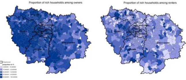
Figure 2: Proportion of rich households among those who move in 1998, by pseudo-commune and tenure status

Source: French Census of 1999

This is consistent withFigure 2, which shows that rich owners are concentrated in Paris and its Western suburbs. By contrast, the concentration of rich households by pseudo-commune is less stringent among renters.

3.3. Extension to heterogeneous preferences and discrete location choice with unconstrained choice set

We now extend the model in several directions in order to make it more realistic.

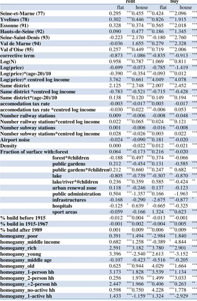
First, households have heterogeneous preferences. This means that the parameters βS _{and γ}S

may depend on household characteristics such as income, household head age and nationality, or household composition (see Table 1 to Table 3). In addition, depending on their characteristics, households may value differently the various components of local amenities z. For example, households with children are more sensitive than singles to parks and other green spaces. This implies that the universal function value function (z), which implicitly assumes that all households agree on the way the local amenities can be aggregated in a single unidimensional function (z), has to be replaced with a household-specific function value

Second, distance to CBD is a poor proxy for commuting costs, which also depend on the structure of the (public and private) transportation network.

As a result, it seems more realistic to replace the continuous variables d and (z) by a discrete list of potential locations, namely the different “communes”.

Table 1: Distribution of location, tenure status and dwelling type for households which moved in 1998 Paris Inner Ring Outer

Ring

Rent flat Own Flat Rent House

Own House

Total 27.58% 36.35% 36.07% 70.79% 13.52% 5.21% 10.48%

Single 38.23% 34.66% 27.11% 81.08% 13.99% 2.74% 2.20%

couple w/o children 27.13% 35.97% 36.90% 69.53% 15.08% 5.28% 10.10%

couple with children 15.64% 38.61% 45.75% 59.92% 11.74% 8.00% 20.35%

Young 28.92% 36.09% 34.99% 79.07% 10.03% 4.49% 6.41% middle-age 25.12% 36.99% 37.89% 60.73% 15.79% 6.82% 16.66% Old 28.54% 35.61% 35.85% 58.30% 25.80% 3.63% 12.27% Poor 26.90% 39.26% 33.84% 83.92% 8.84% 3.86% 3.38% medium income 25.99% 35.52% 38.48% 69.93% 13.09% 5.71% 11.28% Rich 31.03% 33.49% 35.48% 53.35% 20.88% 6.35% 19.43% French 27.24% 35.16% 37.60% 69.10% 14.46% 5.35% 11.09% Foreign 29.53% 43.10% 27.37% 80.38% 8.19% 4.37% 7.06%

Table 2: Distribution of location, tenure status and dwelling type for all households Paris Inner Ring Outer

Ring

Rent flat Own Flat Rent House

Own House

Total 23.24% 37.04% 39.72% 49.45% 21.98% 3.45% 25.11%

Single 35.31% 36.77% 27.92% 60.40% 26.47% 2.11% 11.02%

couple w/o children 20.12% 36.73% 43.15% 40.06% 23.17% 3.04% 33.72%

couple with children 14.15% 37.65% 48.21% 48.02% 16.16% 5.26% 30.56%

young 26.63% 36.96% 36.41% 73.11% 13.90% 4.14% 8.84% middle-age 20.41% 36.73% 42.87% 46.75% 20.18% 4.22% 28.85% old 24.47% 37.49% 38.04% 36.61% 29.79% 2.02% 31.58% poor 24.26% 40.86% 34.88% 63.41% 18.32% 2.89% 15.38% medium income 20.72% 37.16% 42.12% 51.31% 19.81% 3.89% 24.98% rich 25.13% 33.10% 41.77% 33.34% 28.17% 3.51% 34.99% French 22.98% 36.12% 40.90% 46.93% 23.16% 3.42% 26.49% foreign 25.17% 43.83% 31.00% 68.08% 13.25% 3.75% 14.92%

Third, as mentioned in Section 2, there are imperfections in the financial (and real estate) markets, so that renting and buying prices are not perfectly correlated. Furthermore, prices

(per square meter) also vary significantly by dwelling type, in the sense that the prices of flats and houses are not well correlated.

Table 3: distribution of households by tenure status, dwelling type and location Rent flat Own Flat Rent

House

Own House

All households Total 49.45% 21.98% 3.45% 25.11%

Paris 66.49% 32.46% 0.45% 0.60%

Inner Ring 55.61% 23.55% 2.50% 18.33% Outer Ring 33.74% 14.39% 6.10% 45.78%

Movers Total of Movers 70.79% 13.52% 5.21% 10.48%

Paris 82.55% 16.60% 0.55% 0.30%

Inner Ring 75.27% 14.26% 3.35% 7.12% Outer Ring 57.30% 10.41% 10.63% 21.66%

Households are again assumed to choose their tenure status S and their dwelling type T in the first step of the program. In second step of the program, households choose location j in a discrete set. Location determines distance d to CBD and local amenities z. Finally, the quantities of housing and other goods are chosen in the third step of the program. Liquidity constraints are neglected in this section, so that the third step of the program is the same as in Section 3.1, with some obvious change in notation.

Location j is characterized by a series of tenure-specific prices



STj . Eq. (3) is then replaced

with the indirect utility for household i of choosing location j, conditional on tenure S and dwelling type T: ST ij ST j ST i ij ST i ST i j ST i ST ij Z y U 



1  .



2 



3 ln~ 



4 ln







* (11)

where



_kiST

,

k



1

,...,

4

are household-specific preference parameters.

Whereas the rental price of a housing unit is observed, the user cost of a purchased housing unit is not and has to be proxied by the purchasing price. Consequently, in Eq. (3), the use cost



S_j is replaced by the rental price when the dwelling is for rent and by the selling price

represents a multidimensional bundle of observed local amenities which can be valued differently by different households. Similarly to capture the effect of commuting cost on disposable income, a vector Dj of measures of accessibility to location j is interacted with

log-income through the term ln(y ).i Dj which replace

ln

y~

ijin Eq. (6).

One may assume that each household chooses simultaneously the tenure S, the dwelling type T and the location j, that is, the alternative (S,T,j) which provides it with the highest utility. In this case, the probability that alternative (S,T,j) is chosen by household i is given by:

).

Pr(

)

,

,

(

_'' '* ' ,' ,' * ST ij j T S ST ij i

S

T

j

U

Max

U

P





(12)

Under the assumption that the residuals are i.i.d. with a Gumbel distribution, the probability that alternative (S,T,j) is chosen by household i can then be written:

 

 



    J j T S T S ij ST ij i V V j T S P ' ; flat house, ' ; rent own, ' ' ' ' exp exp ) , , ( , (13)

where J denotes the set of locations j. The parameters



_kiST

,

k



1

,...,

4

measuring marginal utilities in the resulting multinomial logit model can then be estimated using standard maximum likelihood techniques.

The drawback of such a joint model is that it relies on the Independence of Irrelevant Alternatives (IIA) hypothesis which stipulates that the choice between two alternatives is not affected by the availability of other alternatives, not by the utility provided by the alternatives. This hypothesis does not seem plausible when households choose both tenure status S, dwelling type T and location j. It seems more relevant to assume that when the alternative (S,T,j) preferred by household i is no more available or becomes less attractive, then household i will primarily tend to select a different location j’ but will tend to still select the same tenure status S and dwelling type T. This tendency is taken into account by estimating a

nested logit model (NL) rather than a multinomial logit model (MNL). More details and justifications are provided in Inoa, Picard and de Palma (2015).

Renting a dwelling is often a temporary alternative before buying one, so that the observable and unobservable characteristics that determine the rent of a dwelling might be different from those that determine the decision to buy a similar dwelling. In particular, the expected future sale price of a dwelling, which is part of the unobservable determinants of its purchase, is irrelevant when renting. Moreover, houses and flats differ in their average size, use cost (lower /no condominium fees but larger real estate taxation and maintenance cost for houses) so that some unobservable determinants might be specific to the dwelling type.

The effect of observed household characteristics on the generic preference for a given tenure status and dwelling type (whatever its location) can be imbedded in the parameter



1STi , both

in the MLN and in the NL model. The fact that the local price in location j is specific to tenure status and dwelling type is imbedded in the price variable ln



ST_j , and the fact that price

elasticity may depend on tenure status and dwelling type is imbedded in the coefficients



₄ST_i (indexed by i to reflect the fact that it may depend on observable household characteristics). Similarly, the fact that the willingness to pay for a better accessibility and for local amenities may depend on tenure status, on dwelling type and on observable household characteristics can be imbedded in the coefficients



₃ST_i and



₂ST_i , both in the MLN and in the NL model. To account for the potential correlation between the error terms by dwelling type and tenure status, a type-tenure-specific error term



iTS and a tenure-specific error term



iSare added to

the equation. They correspond to unobserved heterogeneity of preferences for dwelling type and tenure status. In addition to the type-tenure-specific term



_i1ST, a tenure-specific term



_i1S_,

iS S iT ST ij ST j ST i j i ST i ST i j S i ST i ST ij Z y D U 



1 



1  .



2 



3 ln . 



4 ln















* (14) A nested logit is then estimated for the choice of location, dwelling type and tenure status (Inoa et al. 2013 detail the interpretation of the nested logit).

The deterministic utility of Equation (44) can be split into three additive deterministic utilities: iS S iT ST ij iS S iT ST ij ST ij V V V U *    











(15) with S i iS ST i S iT ST j ST i j i ST i ST i j ST ij a V V D y Z V 1 1 4 3 2 ln . ln .           (16) ST ij

V denotes the deterministic utility provided to household i by location j conditionally on

dwelling type T and on tenure status S,

V

_iTS denotes the deterministic utility provided by

dwelling type T conditionally on tenure status S (whatever location j), and

V

_iS denotes the

deterministic utility provided by the tenure status S (whatever location j and dwelling type T). Under the standard assumptions of a nested logit model, the probability that household i chooses location j conditionally on dwelling type T and tenure status S is given by the usual Multinomial Logit formula:



    ) , ( ) exp( ) exp( ) , ( T S K k ST ik ST ST ij ST i V V S T j P   (17)

The probability that household i chooses a house conditionally on tenure status S according to the logistic formula:





                                   Flat House, , , , . 1 exp . 1 exp ) House ( t S it St S it S S House i House S S House i S i I V I V S T P     (18) where _       



 ( , ) ) exp( ln T S K k ST it ST S iT V

I  is called the inclusive value of the nest K( TS, ) and

corresponds to the maximum utility that household i can expect conditional on choosing tenure S and dwelling type T.

Finally, the probability that household i chooses a house conditionally on tenure status S:





                         Rent Own, , . exp ) . ( exp ) Own ( s is S is iOwn Own Own i i I V I V S P       (19) where _                



 ( , ) exp ln T S K k S iT ST S S iT S S iT V I I  

 is the inclusive value of tenure status S and can be considered as the maximum utility household i can expect conditional on choosing tenure S.

The probability for household i to choose a dwelling j of type T with tenure status S is the product of the three probabilities defined by Eq. (7) to Eq. (9). To estimate the parameters of those equations, one of the scale parameters must be normalized: we choose to normalize that of the total disturbance: 1.

3.4. Extension to constrained choice sets

The coefficients estimated from the nested logit might reflect not only household marginal utilities, but also the liquidity constraints they may face. Indeed, as shown by our structural models, the maximum borrowable value

A

max affects the tenure and location choices when

liquidity constraint on household is binding: on one hand, the marginal disutility of the distance decrease; on the other hand, the utility of ownership compared to tenancy decreases. Moreover, this constraint is likely to modify the choice set faced by households:

i) When the optimal housing consumption that household can afford to buy in location j is lower than the minimal buyable housing service in j then dwellings for sale in j disappears from i’s choice set

ii) When

A

_imax=0 then i can’t buy any dwelling and all the dwellings for sale

disappear from its choice set

Liquidity contraints are then likely to bias the estimation of the marginal utilities by implicitly reducing each household i’s choice set of buyable alternatives to the dwellings whose value is less than

A

_imax.

Constraints on the choice set can be taken into account by distinguishing several choice sets instead of considering only one. Hence, the obtained model is a discrete choice model with latent (or endogenous) choice sets. In such a model, the probability that a household choose a dwelling is not only the probability that this dwelling provides it with the highest utility but also depends on the probability that this dwelling is available to this household.

In this section, we consider the particular case where some households have a maximum borrowable amount equal to zero and extend the previously described nested logit to account for this case. We assume that some households are constrained to rent their dwelling and, consequently, face a choice set which contains only alternatives to rent. The probability to face this choice set is modeled by a binary logit and integrated to the previous nested logit. The previous assumptions about the choice between renting/buying and house/flat still hold so that the location choice among the unconstrained choice set can be modeled by the same

3-opposite, the location choice for constrained households is restricted to the estimation of the two lower levels: the choices of the city and the type of dwelling. The parameters of these latter choices are assumed to be the same whether the household is constrained or not.

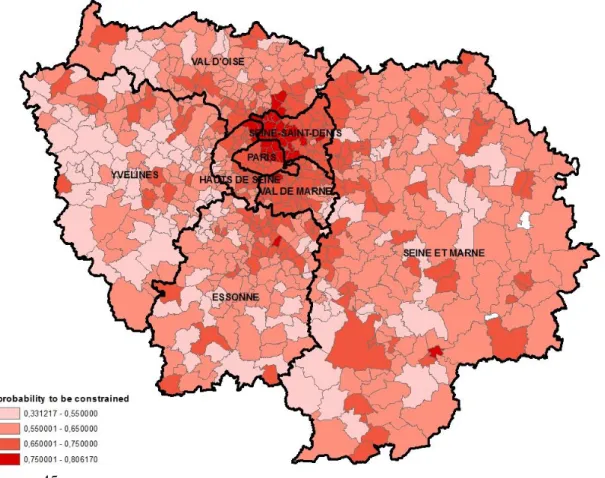
The propensity to be constrained is not observed but inferred from the model by modifying the formula of the probability to buy in the nested logit and maximizing the corresponding likelihood maximization. The probabilities to choose to buy a house become:

) 0 constraint ( ) 0 constraint own ( ) own (   _i    _i  i S P S P P (20) with 



             rent own, " " " " ) . 1 ( exp ) . 1 exp( ) 0 constraint own ( s is sT is s own i S own i i I V I V S P    (21) and ) exp( 1 1 ) 0 constraint (



i i X P    (22)

Distinguishing variables' effect on constraints from their effects on choice is made possible by our definition of latent choice: a variable which influences the household constraint will determine which latent choice set this household will face, while a variable which influences its choice will affect its utility. A same variable can affect both constraint and utility, this might be the case of income for instance.

The case without constraints is represented in Figure 3 and the case with constraints on Figure 4.

Figure 3: Location choice model without constraints

Figure 4: Location choice model with constraints

4. Resul ts

We applied our models to the Paris Region which includes Paris city and its suburbs. The city

Rent Buy House Flat House Flat Commune 1 Commune 1 Commune 1 Commune n Commune n Commune n Commune n Commune 1 Commune 2 Commune 2 Commune 2 Commune 2

...

...

...

...

Rent Buy House Flat House Flat Commune 1 Commune 1 Commune 1 Commune n Commune n Commune n Commune n Commune 1 Rent House Flat Unconstrained Constrained Commune 1 Commune 1 Commune n Commune n

...

...

...

...

...

...

region. The total number of jobs is 5.1 million. The region spreads over 12,000 sq. Km, which represents 2% of the surface of France, but 19% of the population and 22% of the jobs of the country. There are 3 levels of administrative boundaries in Ile-de-France: 1 “région”, 8 “départements” (counties) and 1300 “cities” (communes). In addition, we consider the 3 counties around Paris as close suburb or “inner ring” and the 4 counties far away from Paris as far away suburb or “outer ring”.

We use household exhaustive data from the 1999 French Census for Ile-de-France, which represents about 5 million households. In order to study location choice, we restrict our sample to households who moved in 1998. We exclude households freely hosted and households whose head, so that we obtain a sample of 521,132 households. This database contains rich information on households such as household size, number of children, household head gender, occupation, educational attainment, previous county if residence, and so on. Household (per capita) income is not observed directly, but we computed it as a function of household characteristics, with a very good fit.

Each model is estimated following two steps. The first step is common to both model and consists in estimating a discrete location choice model for each of the four nests (T, S) from the sample of households who actually choose this nest. Each nest is constituted of 725 alternatives corresponding the 725 pseudo-communes7 _{of the Paris region. In order to form}

the inclusive value of each nest (T,S) used in Eq. (8), we compute for each household and each nest the utilities of the 725 alternatives from the coefficients obtained in the first step. By summing up the exponential of utilities and computing the logarithm of this sum, we obtained 4 inclusive values (one by nest) that we use to estimate the parameters in the second step.

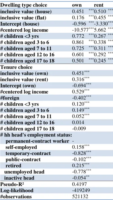
The second step consists in estimating simultaneously the equations of dwelling type choice and tenure choice. Eq. (8) and Eq. (9) are then estimated to determine the parameters of the model without constraints whereas Eq. (8), Eq. (11) and Eq. (12) are estimated for the model with constraints. The inclusive values represent the maximal utility a household can obtain from the set of alternatives contained in nest and constitute additional explanatory variables of the dwelling type choice (Eq. (8)). Other determinants consist in variables which are likely to affect the desired size of dwelling and the income path, such as income per capita, family composition and stability of household head employment.

4.1. Location choice

The estimation of the first step requires not only data on households who moved in 1998 but also some descriptive statistics on local amenities. Based on the aggregation of some variables of the Census by city, we computed local characteristics such as the proportions of poor households, of rich households, of households with one member, with 2 members, etc.

The census data was also used to determine the demands for location in each city by type of dwelling and tenure mode in 1998. Combining those demands with the number of vacant dwellings in each city then allow us with measuring the supply of dwellings by city and by type of dwelling. Whereas the supply of dwellings in Paris and the close suburbs is mainly constituted of flats, the supply in the further suburbs is more balanced between houses and flats, with a particularly high proportion of flats at the East of the Paris region (see figure 14 in appendix). This reinforced the usual assumption in the canonical model that more land can be consumed when locating far from the central business districts.

Local dwelling prices (per square meter) are edited by the Editions Callon in their “yearly guide of venal values” at the city level, separately available for renting and for buying, for flats and for houses. Unfortunately, this guide concerns only cities with more than 5000