Optimal Power Flow Considering Voltage Stability with
Significant Wind Penetration
by
Majid BAVAFA
MANUSCRIPT-BASED THESIS PRESENTED TO ÉCOLE DE
TECHNOLOGIE SUPÉRIEURE IN PARTIAL FULFILLMENT FOR THE
DEGREE OF DOCTOR OF PHILOSOPHY
Ph.D.
MONTREAL, JULY 18
TH, 2017
ÉCOLE DE TECHNOLOGIE SUPÉRIEURE
UNIVERSITÉ DU QUÉBEC
It is forbidden to reproduce, save or share the content of this document either in whole or in parts. The reader who wishes to print or save this document on any media must first get the permission of the author.
BOARD OF EXAMINERS
THIS THESIS HAS BEEN EVALUATED BY THE FOLLOWING BOARD OF EXAMINERS
Mr. Louis A. Dessaint, Thesis Supervisor
Department of electrical engineering, École de technologie supérieure
Mr. Roger Champagne, President of the Board of Examiners
Department of Software and IT Engineering, École de technologie supérieure
Mrs. Ouassima Akhrif, Member of the jury
Department of electrical engineering, École de technologie supérieure
Mr. Pierre Jean Lagace, Member of the jury
Department of electrical engineering, École de technologie supérieure
Mr. Serge Lefebvre, External Evaluator Research Institute of Hydro-Quebec (IREQ)
THIS THESIS WAS PRENSENTED AND DEFENDED
IN THE PRESENCE OF A BOARD OF EXAMINERS AND PUBLIC ON JUNE 29TH, 2017
ACKNOWLEDGMENT
My deepest thanks goes to my supervisor Professor Louis A. Dessaint for his generous advice during the development of my thesis. I have been extremely lucky to have a supervisor who cared so much about my work, and who reviewed my reports so promptly.
I also would like to offer my special thanks to the members of my Ph.D. committee who evaluated my thesis and provided valuable feedback. My special thanks are extended to my colleagues at GREPCI for providing a pleasant work environment.
I would like to express my very great appreciation to my wife Neda, for her love, patience, pushing me when needed. I wish to thank her for encouraging me in all of my pursuits and inspiring me to follow my dreams.
Finally, I am very thankful to my parents for their continuous support and motivation from my home country. They encouraged me to explore correct directions in life and continue with considerable ambition.
FLUX DE PUISSANCE OPTIMALE COMPTE TENU DE LA STABILITÉ EN TENSION AVEC FORTE PÉNÉTRATION DU VENT
Majid BAVAFA
RÉSUMÉ
L'évaluation de la stabilité de la tension est l'un des problèmes majeurs dans le fonctionnement et le contrôle du système d'alimentation. L'une des raisons est le nombre important de chutes de tension qui surviennent fréquemment. L'objectif principal de cette thèse est de choisir un critère approprié pour l'évaluation de la stabilité de la tension dans une approche optimale du flux de puissance (OPF) en considérant la pire contingence possible, ou un état congestionné. La stabilité de la tension peut être affectée par de nombreux éléments et moyens de contrôle qui opèrent à différentes échelles de temps. En particulier, les rôles de la génération d'énergie éolienne, de la réponse à la demande (DR), du limiteur de surexcitation (OXL), du système de stockage d'énergie (ESS) et du changeur de prises (OLTC) sont significatifs. La modélisation appropriée de ces éléments et des moyens de contrôle ainsi que l'utilisation d’une approche OPF devraient être analysés dans des conditions de tension stable sur un long terme.
Tout d'abord, un indice basé sur l'impédance (IB) est présenté dans cette thèse et permet d'évaluer le comportement instable du système d'alimentation intégré à des parcs éoliens avec générateur d'induction doublement alimenté (DFIG). Un modèle pour les limites de la courbe de capacité DFIG pouvant être intégré au circuit interne du générateur est présenté. D’autre part, le modèle OLTC a été ajouté à cet indice. L'indice utilise le concept du circuit à un seul port couplé. L'OPF avec une nouvelle contrainte sur l’indice d’impédance (IB) est implémenté pour démontrer la performance de ce dernier.
Cette étude introduit également une approche du flux de puissance optimale stochastique (SOPF) multi-objectif en présence de génération d’énergie éolienne incertaine. Le SOPF multi-objectif étudie les coûts d'exploitation, la stabilité de la tension et les effets d'émission en tant que fonctions objectifs. L'effet du programme DR est considéré dans cette étude. La technique de fuzzification est utilisée afin de normaliser toutes les fonctions objectifs du SOPF multi-objectif. Un indice de stabilité de tension de ligne (LVSI) est présenté et comparé à d'autres. Le SOPF multi-objectif proposé est également réalisé avec différentes LVSI existantes en tant que fonctions objectifs.
Suite à l'évaluation de la stabilité de la tension, le contrôle de la fréquence est également pris en compte dans le SOPF. Dans ce cas, le procédé de restauration de fréquence coopère avec la DR et la réserve tournante pour arrêter la baisse de fréquence dans les événements de contingence. Ce procédé est défini en trois niveaux. De plus, un indice L (EL) étendu est utilisé pour évaluer l'analyse de la stabilité de la tension. Plusieurs contraintes de fréquence et
de tension sont ajoutées dans l'approche SOPF. L'indice EL considère un modèle équivalent de générateur (GEM). En outre, les systèmes de stockage d'énergie (ESS) sont considérés dans cette approche SOPF.
Ces approches sont analysées en détail, testées et validées sur plusieurs études de cas. Les résultats montrent que l'approche proposée fonctionne avec succès.
Mots-clés : Flux de Puissance Optimale, Indice de Stabilité de la Tension, Réponse à la
OPTIMAL POWER FLOW CONSIDERING VOLTAGE STABILITY WITH SIGNIFICANT WIND PENETRATION
Majid BAVAFA
ABSTRACT
Voltage stability evaluation is one of the major issues in the power system operation and control. One reason is that there is an enormous number of voltage collapses which frequently occurs. The principal objective of this thesis is to choose appropriate criteria for voltage stability evaluation in optimal power flow (OPF) approach considering the worst contingency or the congested condition. Voltage stability can be affected by several elements and control ways which operate on different time scales. In particular, the role of wind power generation, demand response (DR), over excitation limiter (OXL), energy storage system (ESS) and on-load tap changer (OLTC) are significant. The proper modelling of these elements and control ways as well as using in an OPF approach should be analyzed in long-term voltage stability.
First, an impedance-based (IB) index is presented in this thesis that can evaluate unstable behavior of the power system with doubly-fed induction generator (DFIG) wind farms integration. A model for DFIG capability curve limits is presented that can be integrated to the internal circuit of the generator. Furthermore, the OLTC model was added to this index. The index uses the concept of coupled single-port circuit. The OPF with new IB-index constraint is implemented to show the performance of the index.
This study also introduces a multi-objective stochastic optimal power flow (SOPF) approach with the presence of uncertain wind power generations. The multi-objective SOPF investigates the operating cost, voltage stability and emission effects as the objective functions. The effect of the DR program is considered in this study. The fuzzification technique is used to normalize all objective functions in the multi-objective SOPF. A line voltage stability index (LVSI) is presented and compared with other LVSIs. The proposed multi-objective SOPF is also carried out with different existing LVSIs as the objective functions.
Following the voltage stability assessment, the frequency control is also considered in the SOPF. In this case, the frequency restoration scheme cooperates with DR and spinning reserve to stop a frequency drop in contingency events. This scheme is defined in three levels. Furthermore, an extended-L (EL) index is used to evaluate voltage stability analysis. Several frequency and voltage constraints are added in the SOPF approach. The EL-index considers a generator equivalent model (GEM). In addition, energy storage systems (ESSs) are considered in this SOPF approach.
Those approaches are analyzed in detail and they are tested and validated on several case studies. The results show that the proposed approaches operate successfully.
TABLE OF CONTENTS
Page
INTRODUCTION ...1
CHAPTER 1 LITERATURE REVIEW ...11
1.1 Basic principles of voltage stability ...11
1.1.1 Different types of stability and voltage stability ... 11
1.1.2 Operating points and zones ... 13
1.1.3 Voltage stability evaluation methods ... 14
1.1.4 QSS time-domain simulation ... 15
1.2 Evaluation of main effects on voltage stability ...16
1.2.1 Effect of reactive power limits on voltage stability ... 17
1.2.2 Effect of OLTCs on voltage stability ... 19
1.2.3 Effect of load models on voltage stability ... 20
1.3 Methods of solving reactive power dispatch problem ...21
1.4 Analysis of main voltage stability indices ...23
1.4.1 Evaluation of loading margin as global index ... 25
1.4.2 Indices based on singular value method ... 26
1.4.3 Line voltage stability indices (LVSIs) ... 27
1.4.4 Indices based on L-Index ... 31
1.5 Different types of VSC-OPF approach ...34
1.5.1 Power transfer constraint ... 34
1.5.2 Loading margin constraint ... 35
1.5.3 Singular value constraint... 35
1.5.4 L-Index constraint ... 36
1.5.5 LVSI constraint ... 37
1.6 Stochastic Optimal Power Flow (SOPF) ...37
1.6.1 Demand Response (DR) in SOPF ... 39
1.6.2 Energy Storage Systems (ESSs) in SOPF ... 40
1.7 Conclusion ...41
CHAPTER 2 A NOVEL APPROACH TO DYNAMIC VOLTAGE STABILITY ANALYSIS FOR DFIG WIND PARK INTEGRATION ...41
2.1 Introduction ...42
2.2 Background ...45
2.2.1 Impedance matching theory and its application ... 45
2.2.2 DFIG capability curve limits ... 47
2.2.3 VSC-OPF model ... 48
2.3 Proposed impedance-Based index ...50
2.3.1 Model of DFIG reactive limit in improved IB index ... 50
2.3.2 OLTC model in improved IB index ... 53
2.4 Proposed VSC-OPF method ...54
2.5.1 Voltage stability monitoring ... 56
2.5.1.1 Modified WECC test system ... 56
2.5.1.2 Modified IEEE 39-bus system ... 59
2.5.2 VSC-OPF ... 60
2.5.2.1 IEEE 39-bus system ... 62
2.5.2.2 IEEE 57-bus system ... 63
2.5.2.3 Polish 2746-bus system ... 65
2.6 Conclusion ... 66
CHAPTER 3 MULTI-OBJECTIVE STOCHASTIC OPTIMAL POWER FLOW CONSIDERING VOLTAGE STABILITY AND DEMAND RESPONSE WITH SIGNIFICANT WIND PENETRATION ... 69
3.1 Introduction ... 71
3.2 Multi-objective SOPF formulation and constraints ... 74
3.3 Operating points and zones ... 76
3.4 Fuzzification of multi-objective SOPF ... 77
3.5 Line voltage stability index (LVSI) ... 80
3.6 Simulation result and discussion ... 83
3.6.1 Voltage stability monitoring of LVSIs ... 83
3.6.1.1 Modified WECC test system ... 83
3.6.1.2 IEEE 39-bus system ... 86
3.6.2 Multi-objective SOPF ... 87
3.7 Conclusion ... 93
CHAPTER 4 FREQUENCY AND VOLTAGE CONSTRAINED STOCHASTIC OPTIMAL POWER FLOW CONSIDERING WIND POWER AND DEMAND RESPONSE RESOURCES ... 95
4.1 Introduction ... 98
4.2 Background review ... 102
4.2.1 System frequency response model ... 102
4.2.2 Frequency restoration scheme ... 104
4.2.2.1 Level one (frequency below 59.2 ) ... 105
4.2.2.2 Level two (frequency between 59.2 and 59.5 ) ... 106
4.2.2.3 Level three (frequency between 59.5 and 59.7 ) ... 106
4.2.3 EL-Index calculation ... 106
4.3 Proposed frequency and voltage constrained SOPF ... 108
4.4 Numerical analysis ... 112
4.4.1.1 Maximum single contingency ... 113
4.4.1.2 Double contingency ... 115
4.5 Conclusion ... 117
CONCLUSION………..119
APPENDIX I IMPEDANCE MATCHING THEORY ... 123
APPENDIX III IEEE RTS 96-BUS SYSTEM ...127
APPENDIX IV IEEE 39-BUS SYSTEM ...129
APPENDIX V IEEE 57-BUS SYSTEM ...131
LIST OF TABLES
Page
Table 1.1 Different types of VSIs ...23
Table 2.1 Proposed VSC-OPF results for stressed condition (IEEE 39-bus) ...62
Table 2.2 Comparison between different VSC-OPF results for IEEE 57-bus system ...64
Table 2.3 Proposed VSC-OPF for Polish 2746-bus system...65
Table 3.1 Multi-objective SOPF for different LVSIs under scenario #1 ...89
Table 3.2 Active power output of wind farms (MW) under different scenarios ...92
Table 3.3 DR dispatches (MW) under different scenarios ...92
Table 4.1 DR and LS deployment (MW) in double-contingency case ...116
LIST OF FIGURES
Page
Figure 1.1 Different types of power system stability ...12
Figure 1.2 Operating zones in a PV curve ...13
Figure 1.3 Voltage stability evaluation methods ...14
Figure 1.4 Equations of FTS and QSS simulations ...16
Figure 1.5 QSS simulation mechanism ...17
Figure 1.6 Effect of reactive power limit (a) Case I, (b) Case II ...18
Figure 1.7 Different operating points with various load types in a PV curve ...22
Figure 1.8 Comparison between ( ) and ( ) (reactive load increase) ...27
Figure 1.9 A two-bus power system ...28
Figure 1.10 Comparison between voltage collapse proximity indicators ...29
Figure 1.11 Power system model with m PV bus and k Loads (L Index)...32
Figure 1.12 Power system model with m PV bus and k Loads (Extended L Index) ....33
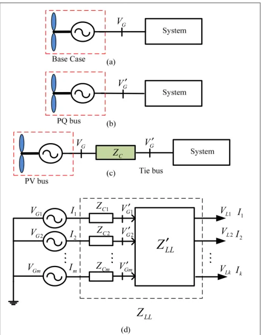
Figure 2.1 Modeling of the DFIG reactive limit (a) Base case (b) After DFIG reactive limit. (c) Modified system (d) Modified multi-port power system with considering proposed model ...52
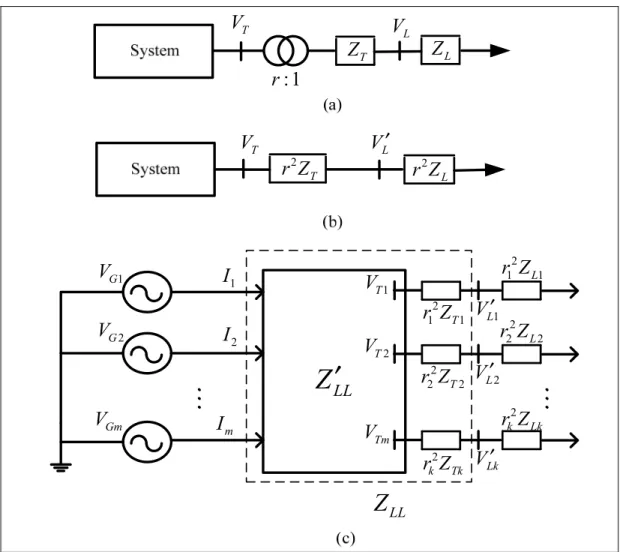
Figure 2.2 Modeling of the OLTC (a) System with OLTC (b) Modified system ...54
Figure 2.3 Flowchart of the proposed VSC-OPF method ...55
Figure 2.4 Modified WECC test system ...57
Figure 2.5 Voltage instability in modified WECC system (a) Voltage magnitude at buses 3 and 4 (b) Tap changing in the OLTC (c) Comparison of IB indices at the load ...58
Figure 2.6 Voltage instability in modified IEEE 39-bus (a) Voltage magnitude at buses 3, 7 and 40 (b) Tap changing in the OLTC (c) System and load impedances at bus 40 ...61
Figure 2.7 Voltage instability in modified IEEE 39-bus with SVC (a) Voltage magnitude at buses 3, 7 and 40 (b) Comparison between proposed and traditional index ... 62 Figure 2.8 Improved IB index values in the IEEE 39-bus system ... 63 Figure 2.9 Comparison between Different variables in IEEE 57-bus system (a)
Generated reactive power (MVAR) (b) Active power losses (MW) (c) Maximum values of improved IB index (d) Fuel cost function (K$/h) .... 64 Figure 2.10 Sorted improved IB index values in the Polish 2746-bus system ... 65 Figure 3.1 Operating zones (a) PV curve for a load bus (b) Emission curve for a
conventional generator (c) Cost curve for a conventional and wind
generator ... 78 Figure 3.2 Fuzzy membership functions (a) Using for a SOPF objective function
that should be maximized (b) Using for a SOPF objective function that should be minimized ... 79 Figure 3.3 IBLVSI model in a sample power system (a) Two buses of
transmission line ... 80 Figure 3.4 Flowchart of the proposed multi-objective SOPF approach ... 82 Figure 3.5 Modified WECC test system ... 84 Figure 3.6 Modified WECC 9-Bus (a) Voltage magnitude at buses 3 and 4 (b)
Tap changing in the OLTC (c) Comparison of LVSIs ... 85 Figure 3.7 Modified WECC 9-Bus with blocked OLTC (a) Voltage magnitude
at buses 3 and 4 (b) Comparison of LVSIs ... 87 Figure 3.8 IEEE 39-bus system (a) Voltage magnitude at buses 3, 7 and 8 (b)
Comparison of LVSIs (c) IBLVSI behavior ... 89 Figure 3.9 Single/multi-objective SOPF under scenario #1 (a) Comparison of
active power schedule in case 1 & 2 (b) Comparison of voltage
magnitude of buses in cases 1 & 2 ... 91 Figure 4.1 Three-level frequency response curves after contingencies ... 103 Figure 4.2 DR deployment of buses cooperated in DR program for three cases ... 112 Figure 4.3 Voltage magnitude of buses in area three for three cases under
Figure 4.4 Spinning reserve and FIR under scenario #1 ...114 Figure 4.5 Variation of DR deployment with 5% inc/decrement in wind power
penetration...114 Figure 4.6 State of charge in ESSs during 24 hours under scenario #1 ...115 Figure 4.7 Comparison between the costs in different cases in single and ...117
LIST OF ABREVIATIONS
AVR Automatic Voltage Regulator
CCPs Carbon Capture Plants
CPF Continuation Power Flow
DAEs Differential Algebraic Equations
DFIG Doubly Fed Induction Generator
DR Demand Response
ED Economic Dispatch
ENVCI Equivalent Node Voltage Collapse Index EPSO Enhanced Particle Swarm Optimization ESSs Energy Storage Systems
FIR Fast Instantaneous Reserve
FRC Fully Rated Converter
FTS Full Time Scale
FVSI Fast Voltage Stability Index
GA Genetic Algorithm
GEM Generator Equivalent Model GSA Gravitational Search Algorithm
GSC Grid-Side Converter
HDE Hybrid Differential Evolution
IB Impedance Index
LFF Load Flow Feasibility LMPs Local Marginal Prices
LS Load Shedding
LVRT Low Voltage Ride Through LVSI Line Voltage Stability Index
MSV Minimum Singular Value
OLTC On-Load Tap Changer
OPF Optimal Power Flow
OXL Over Excitation Limiter
PF Power Flow
PIs Performance Indices
PMUs Phasor Measurement Units
PSO Particle Swarm Optimisation
QSS Quasi Steady State
RESs Renewable Energy Sources
RPD Reactive Power Dispatch
RSC Rotor-side converter
SFR System Frequency Response
SIR Sustained Instantaneous Reserve
SOC State of Charge
SOPF Stochastic Optimal Power Flow
SVC Static VAR Compensator
TH Threshold Value
TV Tangent Vector
UFLS Under-Frequency Load Shedding
VCPI Voltage Collapse Proximity Indicator
VSC-OPF Voltage Stability Constrained Optimal Power Flow VSM Voltage Stability Margin
WECC Western Electricity and Coordinating Council
WF Wind Farm
INTRODUCTION
Nowadays, voltage stability assessment is an important issue in power systems due to a large number of blackouts in different countries. The main goal of an independent system operator (ISO) is to run the power system operation without any voltage stability collapse at low cost or high revenue. Many voltage stability indices (VSIs) have been presented that have a role to evaluate the voltage instability risk and to predict the voltage collapse point.
In the recent decades, the electric power industry has changed from the monopoly which was controlled by a government to a free competition environment. Many regulations have been changed to be adaptable to this new environment in different areas. Thus, voltage stability assessment carried out by an ISO should be revised and reformulated. It is an undeniable fact that the power system should operate close to the limits of stable conditions, because of minimizing the total costs. Therefore, some factors will be come out which may trigger the long-term voltage instability such as a stressed power system, insufficient fast reactive power resources, on-line load tap changers (OLTCs) response and so on. Several elements have an impact on the voltage control which are OLTCs, generators, over excitation limiters (OXLs), static and switchable capacitor/reactor banks and static VAR control (SVC) (Canizares, 2002).
Voltage instability is a local and a nonlinear phenomenon. When a high voltage variation occurs, the power system may lose the loads in some areas or the elements such as transmission lines and generators (Cutsem et Vournas, 1998). The sequence of cascading events with voltage instability may result in a phenomenon which is named voltage collapse. The outcome of this phenomenon is a blackout or a low-voltage operation. Most reasons of voltage collapse are based on failing to provide reactive power demands (Canizares, 2002; Eremia et Shahidehpour, 2013):
• Inability to provide reactive power by generators and SVC due to the reactive power limits;
• Increase of reactive power loss on the congested transmission lines; • Behavior of OLTCs until hitting their limits;
• Increase of active power loading; • Dynamics of load recovery;
• Contingencies such as line tripping or generator outage.
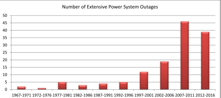
The voltage collapse events can cause extensive power system outages. Thus the number of power system outages worldwide, which are increasing yearly, should be reduced. Figure 0.1 presents a summary of extensive power system outages over the recent half-century. Figure 0.2 shows the approximate percent of extensive outages over the recent half-century based on different locations as the US & Canada, Europe, and the rest of the world (International)(Wikipedia, 2017). Whole outage costs are approximately calculated $75B annually in the US & Canada (McLinn, 2009).
Figure 0.1 Number of extensive power system outages in worldwide
An optimal power flow (OPF) approach was first developed in 1962 by Carpentier. There are different linear and nonlinear solution methods for this approach while linear methods are inaccurate and nonlinear methods are slow and fragile. It is important to get accurate
0 5 10 15 20 25 30 35 40 45 50 1967-1971 1972-1976 1977-1981 1982-1986 1987-1991 1992-1996 1997-2001 2002-2006 2007-2011 2012-2016
solutions because of solving the OPF periodically each five minutes. In spite of the introduction of the OPF more than a half-century, the OPF encounters inaccurate and fragile solutions which may enforce an extra cost in billions of dollars per year to ISO (Cain, O’Neill et Castillo, December, 2012).
Figure 0.2 Percent of extensive power system outages in different locations
Generally, the power flow (PF) analysis shows the behavior of elements in steady state conditions. This analysis can calculate whether power system elements can satisfy the limits in steady state conditions without any contingencies or not. Moreover, the OPF analysis can reach the losses at the minimum level by calculating all the values of voltages and currents (Andersson, 2004). Variations of unpredicted resources like wind power create a high amount of uncertainties. In this situation, stochastic OPF (SOPF) can reduce the risk of outages (Bienstock, Chertkov et Harnett, 2014). The SOPF approach provides an applicable model for uncertainties in the system.
Motivation and Challenges
43%
20% 38%
One of the challenges in power systems is a large number of voltage collapses which frequently occur. Therefore, voltage stability evaluation becomes crucial in power system operation and control. Voltage stability can be affected by several elements and controllers which operate in different time scales. In particular, the role of wind power generation, demand response (DR), over excitation limiter (OXL), on-load tap changer (OLTC) and generator model are significant. The proper modelling of these elements and controllers as well as using an OPF approach should be analyzed for long-term voltage stability.
VSIs can be mixed with OPF and they produce a problem which is named Voltage Stability Constrained OPF (VSC-OPF) (Avalos, Canizares et Anjos, 2008; Canizares et al., 2001; Lage, da Costa et Canizares, 2012; Milano, Canizares et Invernizzi, 2005; Rosehart, Canizares et Quintana, 2003a; 2003b; Venkatesh, Arunagiri et Gooi, 2003). These traditional VSC-OPF approaches don’t consider the model of elements and efficient control ways like wind power generation, DR, OXL, OLTC and generator. Due to the dynamic behavior of power systems, using traditional VSI is not accurate and cannot predict the unstable operating point. Thus, the creation of new VSC-OPF approaches can be useful to improve the performance of ISOs.
Research Objective
The principal objective of this thesis is to choose an appropriate criteria for voltage stability evaluation in SOPF approach and to consider the worst contingency or the congested condition. Modeling of elements and control ways like a wind generator, DR, OXL and OLTC is considered in the OPF formulation.
According to the literature review and simulations that will be described in detail, the following objectives are derived from the principal goal:
• To evaluate and compare several important voltage stability indices; • To compare different VSC-OPF approaches and represent their drawbacks;
• To introduce a novel voltage stability index that can model OLTCs, capability curve limits of traditional generators and wind generators;
• To develop a new formulation for VSC-OPF approaches with the novel voltage stability index;
• To analyze SOPF approaches with the presence of uncertainties in wind power generation;
• To investigate DR and load shedding (LS) program in SOPF approaches;
• To add a frequency restoration scheme in VSC-SOPF formula and find the effects of DR and LS program;
Methodology
The following section describes the proposed methodology to achieve the research objectives. The methodology includes the following steps:
• Comparison between different voltage stability indices such as L-index, minimum singular value and line voltage stability indices (LVSIs) is carried out. Then, VSC-OPF approaches with these indices is implemented in MATLAB and validated in several case studies. The approaches are optimized with different objective functions like minimization of the operating cost function.
• Investigating the behavior of elements and control ways, such as DR, wind generator, OLTC and OXL in the long-term voltage stability simulation with PSAT. This step will help to define new voltage stability indices for better voltage instability detection. Then, implement the VSC-OPF approach with these new indices in MATLAB and PSAT. This approach will be performed in different test systems.
• Implementing SOPF to model the uncertainties in wind power generation. A literature review is done to choose an appropriate technique to consider the uncertainties. • Appending frequency constraints in the VSC-SOPF. These constraints are extracted
program and reserve is considered in this scheme. Due to the complexity and nonlinearity of the constraints, this approach is carried out in GAMS.
Thesis Contributions
The contributions of the thesis are described as follows:
An improved impedance-based index for voltage stability analysis
An improved impedance-based (IB) index is proposed in this thesis that models doubly-fed induction generator (DFIG) capability curve limits and OLTC behavior. These factors have significant roles in the long-term voltage stability studies. The proposed IB index can detect precisely the voltage collapse, especially after the occurrence of a given contingency due to the dynamic elements of the system. It can model the DFIG reactive power capability characteristics as a variable virtual impedance which is adaptable in the dynamic studies. Therefore, the model of DFIG reactive limits can be integrated to the internal circuit of the generator and it can be appended to impedance matching theory. An OLTC model is also added to this index. The OLTC can affect both Thevenin equivalent impedance and load impedance. Thus, the IB index equation is modified by considering those impedance variations on the OLTC model. The robustness of the proposed method has been investigated by including SVC and different load types in the power systems.
A new VSC-OPF approach with proposed improved IB index
A VSC-OPF approach is studied including an improved IB index. A new approach is compared with three existing VSC-OPF approaches in stressed and single line outage conditions. These VSC-OPF approaches are, namely, based on the L-index, the minimum singular value and the voltage collapse proximity indicator (VCPI). The proposed VSC-OPF
approach can reduce the operating cost and the number of voltage collapses. Thus, it can improve the performance of the electric utilities.
A novel LVSI as a criterion for voltage stability detection
This thesis proposes a LVSI which can detect precisely the voltage collapse in comparison with other LVSIs, especially after the occurrence of a given contingency due to the dynamic elements of the system. This index is based on the impedance theory which is a proper way to estimate the maximum power transferred to a load bus. The impedance seen at two buses of a transmission line can provide important information for the operation and control of the power system.
A multi-objective SOPF approach with the presence of uncertain wind power generations
The thesis also implements a multi-objective SOPF approach which consists of the operating cost, voltage stability and emission effects as the objective functions. The wind uncertainty is formulated as a scenario-based technique. DR program is considered in this study, which is one of the most efficient control ways to reduce the risk of voltage instability after a contingency occurrence or a stressed loading condition. In addition, the proposed approach uses the technique of fuzzification to normalize all objective functions and to find the optimal solution. A comprehensive comparison between different LVSIs as the objective function is given in the multi-objective SOPF. Also, the multi-objective SOPF with proposed LVSI is investigated under different scenarios. It can reduce the operating cost and increase the minimum voltage magnitude. Thus, it can improve the performance of the electric utilities.
Frequency and Voltage Constrained SOPF Considering Wind Power and Demand Response Resources
An approach for frequency and voltage control in SOPF with the presence of uncertain wind power generations and energy storage systems (ESSs) is proposed in this thesis. The proposed scenario-based SOPF utilizes a combined DR, ESS, LS and reserve to increase
reliability under various contingency occurrences. The objective function is the minimization of total operating cost and it considers costs for DR, LS, wind spillage and reserve resources. To solve frequency instability issue, it uses the reduced-order system frequency response (SFR) model and creates some extra constraints to be added to the SOPF. The frequency restoration scheme is defined in three levels. To keep a system safe from the viewpoint of voltage stability issue, it uses extended L-index (EL-index).
Thesis Outline
This thesis is organized as follows. Chapter 1 contains a literature review on the impact of different elements on voltage stability analysis and it also presents different VSIs, VSC-OPF and SOPF approaches. Chapter 2 describes a new VSC-OPF approach with proposed improved IB index. The index can model the great changes during a voltage collapse process such as line tripping, load tap changing and reactive power limits of DFIG and conventional generator. This index can also monitor online voltage stability. The proposed IB index can model the DFIG reactive power capability characteristics as a variable virtual impedance which is adaptable in the dynamic studies.
An OLTC model is also added to this index. The OLTC can affect both TEI and load impedance. Thus, the IB index equation is modified by considering those impedance variations on the OLTC model. A new VSC-OPF is also carried out with the proposed IB index. The proposed VSC-OPF can reduce the operating cost and the number of voltage collapses. Thus, it can improve the performance of the electric utilities.
In Chapter 3, a multi-objective SOPF approach with the presence of uncertain wind power generations is investigated. This chapter proposes a multi-objective SOPF problem considering wind uncertainty and DR. This multi-objective SOPF consists of the operating cost, voltage stability and emission effects as the objective functions. Furthermore, a new LVSI is presented that can detect precisely the voltage collapse in comparison with other LVSIs. Finally, a comprehensive comparison between different LVSIs as the objective
function is given in the multi-objective SOPF. Also, the multi-objective SOPF with proposed LVSI is investigated under different scenarios. It can reduce the operating cost and increase the minimum voltage magnitude. Thus, it can improve the performance of the electric utilities.
Chapter 4 includes a frequency and voltage constrained SOPF considering wind power and demand response resources. The proposed scenario-based SOPF utilizes a combined DR, ESS, load shedding (LS) and reserve to increase reliability under various contingency occurrences. In the proposed frequency and voltage stability assessment, the objective function is the minimization of total operating costs and it considers costs for DR, LS, wind spillage and reserve resources. To solve frequency instability issues, this chapter uses the reduced-order system frequency response (SFR) model and creates some constraints to be added to the SOPF. To keep a system safe from the viewpoint of voltage stability issues, it uses the EL-index. The EL-index is one of the voltage stability indices that can predict voltage collapse accurately. Finally, a conclusion and future works are presented at the end of this document.
CHAPTER 1 LITERATURE REVIEW 1.1 Basic principles of voltage stability
This section contains a summary in subjects such as different types of stability, voltage stability evaluation methods, important operating points and QSS time domain simulation.
1.1.1 Different types of stability and voltage stability
The behavior of power system stability changes dynamically and all dynamic systems are based on complicated mathematical equations. From an economical viewpoint, a power system cannot be stable for any perturbations. When a perturbation appears, power system variables such as bus voltages, and machine rotor speeds, active and reactive power will change greatly. These variations activate all governors and voltage regulators to restore a power system to the equilibrium point. Even some elements may be disconnected from network to preserve the main system from cascading instability (Kundur et al., 2004).
Power system stability can be categorized in several forms based on: 1) main variables of the power system; 2) extent of the perturbations; 3) time scales of simulation. Figure 1.1 shows the main types of the power system stability (Canizares, 2002). Long-term voltage stability includes slow dynamic elements such as OLTC, OXL, and some controlled loads. The time scale of this voltage stability is until several minutes. Different forms of instability may change from one form to another in the power system dynamically. To realize the instability forms, it needs to be familiar with dynamic operation behavior of power systems (Kundur et al., 2004). Long-term voltage stability can be divided into large-disturbance and small-disturbance voltage stability. The small-small-disturbance voltage stability problem can be modeled with linearized power system equations with acceptable error. But it cannot disregard nonlinear behavior of some elements such as OLTC. Increasing the active and reactive power
in the inductive elements has a major effect on voltage reduction. Over excitation and under excitation limits of generators or synchronous compensators may intensify this process of voltage reduction when a fault causes and also when the reactive power is not sufficient. In addition, transferring the reactive power for long distance is improper. It has a negative effect on active and reactive power losses and it increases the risk of voltage collapse (Taylor, Balu et Maratukulam, 1994).
Figure 1.1 Different types of power system stability
When the short-term dynamics have diminished, the long-term dynamics (slow dynamics) will remaines and it should be considered. Long-term (LT) voltage instability is classified into three types of instability (Canizares, 2002; Cutsem et Vournas, 1998). LT1 is loss of equilibrium. This instability is the most common instability procedures; load restoration and OLTCs affect on this instability. LT2 is a lack of attraction towards a stable equilibrium. For instance, first LT1 occurs and then corrective actions are performed with a delay. Therefore, there is not enough time to restore the operating point. LT3 is a slow growth of the voltage
oscillation. This instability is less common; one example can be produced by the cascaded load restoration or incorrectly tuned OLTCs.
1.1.2 Operating points and zones
One of the methods for evaluation of voltage stability is continuation power flow (CPF) which produces some curves such as PV, PQ and QV curves. Different types of operating zones represented in Figure 1.2 are divided into the controllable zone and uncontrollable zone in the PV curve. Controllable zone (stable operating zone) is the upper part of the curve. All points of this zone have negative sensitivities. It can be defined as two sub-zones for better evaluation (optimal and critical zones). Uncontrollable zone (unstable operating zone) is the lower part of the curve. All points of this zone have positive sensitivities (Eremia et Shahidehpour, 2013). 2 V 2,max V 2,min V 2,cr V 2 P 2,max P
Figure 1.2 Operating zones in a PV curve
The range of these zones is dependent on different system topology and ISO regulations. For example, as reported by Western Electricity and Coordinating Council (WECC), a safety margin in case 1 (N-0, N-1 contingencies) and case 2 (N-2, N-3 contingencies) are 5% and 2.5%, respectively (Al Dessi, Osman et Ibrahim, 2013).
1.1.3 Voltage stability evaluation methods
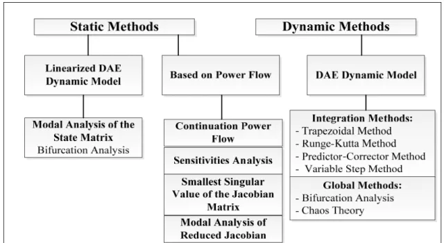
Voltage stability evaluation methods are divided into two fundamental methods which are named static and dynamic methods. Static methods are based on PF equations and linearized differential-algebraic equations (DAEs); also they are considerably quicker than the dynamic methods. Some indices (local or global) are introduced in these methods which will be described in detail. The dynamic methods based on DAEs are divided into the integration and global methods.
Figure 1.3 Voltage stability evaluation methods Adapted from Eremia and Shahidehpour (2013)
The bifurcation theory assumes that variations of system parameters are slow and also it can evaluate the behavior of a system until reaching instability. The power system equations in the bifurcation analysis are defined as states and parameters. The states such as magnitudes and angles of bus voltage, and machine angles change very fast. The parameter changes slowly in the power system equations such as active power demands. How to choose states and parameters are significant in the power system modeling (Canizares, 2002).
Saddle node bifurcation is defined when PF solutions will change until vanishing the convergence. Therefore, there are no PF solutions at this point. Singularity induced bifurcations is defined when the singularity appears in the DAEs of a power system because of changing a state parameter gradually, and then the system immediately falls into instability by an infinite behavior. Voltage instability due to the reactive power limit of generator can be caused the singularity induced bifurcation (Gomez-Exposito, Conejo et Canizares, 2008; Ilić et Zaborszky, 2000).
1.1.4 QSS time-domain simulation
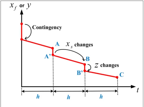
The QSS approach relies on the time-scale decomposition in the long-term dynamics. This approach is a well-known technique which can increase the computational efficiency and also it can be used in the real time voltage assessment. The QSS simulation analyses the long-term instability dynamics and ignores the short-term dynamics. In addition, it can change the value of step size for reaching the optimum time and accuracy (Van Cutsem et Vournas, 1996). The power system dynamics can be divided into continuous and discrete-time parameters because the components (controllers and protecting devices) can be operated based on both continuous and discrete-time state vectors. Based on the above considerations, equations of Full Time Scale (FTS) simulation and QSS simulation are provided in Figure 1.4.
The algebraic function represents the network equations. The differential function relates to some components which can be divided into two sub-functions where is the “slow” state vector, is the “fast” state vector. The algebraic function ℎ shows the discrete events like as capacitor switching, OLTC and OXL operation. As seen in Figure 1.5, parameter ℎ is defined as the time step size of the algorithm (about 1s to 10s) and each dot shows a short-term equilibrium point.
0
( , , )
( , , )
(
1)
( , , ( ))
g x y z
x
f x y z
z k
h x y z k
=
=
+ =
0
( , , , )
0
( , , , )
( , , , )
(
1)
( , , , ( ))
f s f f s s s f s f sg x x y z
f x x y z
x
f x x y z
z k
h x x y z k
=
=
=
+ =
Figure 1.4 Equations of FTS and QSS simulations
Some components like as OXLs, OLTCs and switched shunt elements can act as discrete dynamics, so vertical jumps (A to A’, B to B’) show this behavior. Horizontal jumps (A’ to B, B’ to C) can be obtained from the differential equations and the load self-restoration (Van Cutsem et Mailhot, 1997). The comparison between QSS and FTS simulations is presented in (Gear, 1971) that shows two curves are approximately same and cannot simply be distinguished. The extended QSS model presented in (Grenier, Lefebvre et Van Cutsem, 2005) considers the long-term frequency dynamics. It is useful for the frequency analysis due to large disturbances and also it shows the interaction between frequency and voltage.
1.2 Evaluation of main effects on voltage stability
The voltage stability can be affected by several elements and control ways which operate on different time scales. In particular the role of OLTCs, loads and reactive power limits are significant.
s
x
t
fx
y
z
Figure 1.5 QSS simulation mechanism
1.2.1 Effect of reactive power limits on voltage stability
One of the major impacts on voltage instability is the reactive power limits which are produced by the generators excitation limiters. The system will lose voltage control of generators when the reactive power limits become active (Canizares, 2002). Two examples of PV curves are provided in Figure 1.6(a), when these limits are on or off. In the case I, the reactive power limit decreases the stability margin because the distance between point B and the critical point is decreased. If the load increases in this situation, the point B will reach to the critical point and the voltage instability can be triggered easily. In the case II, the operating point becomes instantly unstable after considering the reactive power limit. As seen in Figure 1.6(b), when the limit is considered, the equilibrium point becomes in the lower part of the constrained PV curve which is unstable. A generator with no reactive power limit is considered as a PV bus, and then a PV bus will change into a PQ bus after involving to the reactive power limit.
2 V 2 P (2) 2max P (1) 2max P (2) 2cr V (1) 2cr V 2 P (2) 2max P (1) 2max P 2 V (2) 2cr V (1) 2cr V
Figure 1.6 Effect of reactive power limit (a) Case I, (b) Case II
There are different models for the representation of reactive power limits of generators in the voltage stability and electricity market studies. One of the most common models is the consideration of the reactive power limits as a fixed value in an OPF approach, but this model is not very accurate due to the nonlinear characteristics of the constraints. Another model can be improved by applying a complete model of generator capability limits. This model considers the maximum currents of field and the maximum currents of stator in its formula. The following represents this model of maximum reactive power limits:
= − − (1.1)
= ( ) − (1.2)
where and represent the reactive power limits for maximum field currents and maximum stator currents, respectively.
Results in (Tamimi, Canizares et Vaez-Zadeh, 2010) show that the model in (1.1)-(1.3) acts better than fixed values of reactive power limit due to providing a improved voltage profile and less power losses. If we want to use other models, it is very important to understand, whether the improvement of voltage profile is more valuable rather than the increase of computational burden or not. Moreover, this model is appropriate model for cylindrical rotor and it can be used for salient pole rotor due to conservative consideration.
1.2.2 Effect of OLTCs on voltage stability
The OLTCs have an important role on voltage stability and they may trigger the instability process. The tap ratio can be changed via manual or automatic procedure. Some OLTCs operate accompany with an automatic voltage regulator (AVR) in power systems, so this action worsen the procedure of voltage instability. The behavior of OLTC equipped with AVR can be presented by two models (discrete or continuous). OLTCs generally operate after a pre-specified delay, and then the tap ratio keeps constant the load side voltage (Weedy et al., 2012).
There are some ways to control the voltage stability by OLTCs which is known as corrective actions. These corrective actions used to control the restoration schemes after a contingency which have negative impacts on voltage stability problem. These are classified into groups below (Vournas et Karystianos, 2004): 1) Tap blocking behavior of an OLTC. One of the easiest methods is the tap blocking of an OLTC which ends to the continuation of the voltage instability. It has some disadvantages such as decreasing the voltage level in both the transmission and distribution system and producing the negative effect on other load restoration processes. Also, it is hard to prevent unnecessary tap blocking and it has a problem in finding which tap needs to be blocked. 2) Specific tap or voltage switching of an
OLTC. This method avoids the continuation of voltage reduction from a specific value. It can be limited by a specific tap ratio or a reference value of the voltage. These values can obtain from the highest probability of contingency or the operator experiences. 3) Tap reversing behavior of an OLTC. This way operates to control the voltage level in both the distribution and transmission sides. An OLTC wants to keep the voltage magnitude at an acceptable level. It causes to prevent the voltage collapse.
The tap reversing behavior avoids the voltage reduction and operates more profitable than other corrective actions. Tap reversing behavior of an OLTC provides enough time for a system to employ other corrective actions. There are some methods to optimize an OLTC setting such as the gradient projection method which is based on maximizing the stability margin (Polak, 1971; Vournas et Karystianos, 2002). In (El-Sadek et al., 1999), a case study is analyzed as a Thevenin’s equivalent system which E is an equivalent Thevenin’s emf and is the load node voltage. Then a criterion (El-Sadek et al., 1997) is introduced as an analytical factor to evaluate the behavior of OLTCs. Note that tap ratio does not change the maximum active and reactive power of a load.
Furthermore, finding the critical OLTCs can help to improve the voltage stability problem. In (Thukaram et Parthasarathy, 1996; Thukaram et al., 2004), the linear programming method has been applied to solve two objective functions which are the minimization of the voltage deviations from desired values and the minimization of the sum square of L-indices. Thus, these methods can show the critical OLTCs which may lead to the voltage instability under the peak load conditions.
1.2.3 Effect of load models on voltage stability
Some elements can intensify the effects of load on voltage stability, such as OLTCs, voltage regulators, thermostats and motor slip adjustments. Restored loads consume more and more reactive power which it cuts down the voltage magnitudes. Moreover, different types of load models have impacts on the voltage stability problem (Lee et Lee, 1993; Pal, 1992; Zeng,
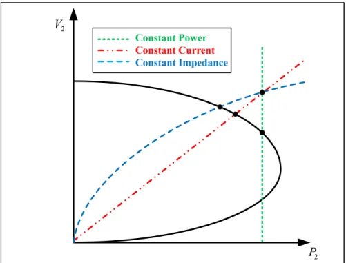
Berizzi et Marannino, 1997). It is beneficial for the electricity industry to develop dynamic load models instead of conventional load models. Note that only dynamic systems have the unstable behavior (Hatipoglu, 2014). (Pal, 1992) proposes an accurate load model with a constant MVA characteristic. The dynamic behavior of this model is indicated by a first-order delay term. (Chowdhury et Taylor, 2000) compares between two methods of stability evaluation (QV curve obtained from the conventional PF approach and the dynamic simulation). This paper evaluates three worst outages which are stable in the dynamic simulation, but they are unstable by the PF approach and there is no operating point in the QV curve. Thus, the results of the PF approach are not reliable. Well-known curves such as PV and QV curves cannot consider the dynamic load characteristics, because they are not time-dependent. In (Lian et al., 2010), the authors propose a method to consider the dynamic load characteristics. It first converts a power system into an equivalent two-node system and then an approximated method is used to model the dynamic load with a polynomial form. Figure 1.7 represents that different types of load models have distinct operating points. It shows that constant impedance (Z), constant current (I) and constant power (P) load models have significant impacts on the voltage stability problem due to different intersections in the PV curve.
(Regulski, 2012) investigates a voltage stability evaluation in different load characteristics. When a contingency occurs, some loads act quickly and reach to new operating points, while others act with delay. In the case of a constant power load, an operating point may be vanished; when it passes maximum active power limit. Thus, consideration of fixed value for the load model creates many errors in the voltage stability results.
1.3 Methods of solving reactive power dispatch problem
The reactive power dispatch (RPD) problem tries to keep the voltages in acceptable values. There are some control variables which are needed to optimize such as generator parameters, switchable VAR sources and OLTCs. As discussed in (Thukaram et Parthasarathy, 1996;
Thukaram et al., 2004), the authors use the linear programming method to solve this problem. The RPD problem can be solved by Genetic Algorithm (GA) which the RDP objective function is the minimization of the maximum of L-indices for all buses (Devaraj et Roselyn, 2010). The hybrid differential evolution (HDE) is another heuristic method which solves the RDP optimization (Yang et al., 2012). This technique can obviously enhance the voltage stability of a system and reduce the line losses. Also, it can determine the optimal tap settings of OLTCs, the excitation settings of generators and the locations of the SVCs.
In (Wang et al., 2011), a new enhanced particle swarm optimization (EPSO) is presented for solving a preventive control. The new EPSO has a difference with PSO in the selection of inertia weight. Moreover, a gravitational search algorithm (GSA) is introduced to solve the RPD problem in (Duman et al., 2012a). GSA is a new metaheuristic search algorithm and motivated by Newtonian gravitational law and law of motion (Rashedi, Nezamabadi-pour et Saryazdi, 2009). In this algorithm, a heavier mass has a higher pull and moves slower.
2 P 2
V
1.4 Analysis of main voltage stability indices
One of the useful methods to evaluate the voltage instability risk is the calculations of voltage stability indices (VSIs). These indices usually calculate the stable operating point which is obtained from load flow feasibility (LFF). They are also identified as performance indices (PI) which are an interesting topic for the researchers in the power system operation. A threshold value (TH) as a measurement criteria is defined for each VSI (Chow, Fischl et Yan, 1990). When ( , ) ≤ , the voltage profile is adequate and when ( , ) >
, the voltage profile is inadequate. Where is a reference value of , and ( , ) is obtained from a group of variables that produces the operating point . Some of these VSIs are introduced in Table 1.1.
Table 1.1 Different types of VSIs
Adapted from Fischi (1989) and, Eremia and Shahidehpour (2013)
Criterion of Index Formulation Explanation
Maximum power transfer (Barbier et Barret, 1980)
∈
( ) ≤
where is the voltage magnitude at load bus ; is the critical voltage magnitude at bus
Critical voltages of load bus calculated based on maximum power transfer limit,
= 1.0 Maximum power
transfer from OPF (Carpentier, 1984)
∈ ( ) ∗ ≤ (Selected by operators)
where is the total reactive power generation, is defined from optimal power flow (∗)
A voltage collapse sensitivity index based on maximum power transfer criteria and computed from an optimal power flow Load flow feasibility
(Jarjis et Galiana, 1981)
1
sin([ ], [ ]) ≤
= + (1 − )
where is the base case input vector; is the closest input vector boundary of load flow region from ; k is a positive integer;
At boundary of load flow feasibility region = ∞
Load flow (L-Index) (Kessel et Glavitsch, 1986) ∈ 1 − ∑∈ ≤
where is the load bus voltage magnitude of bus ; and is the elements of the matrix, [ ]= −
At boundary of load flow feasibility region = 1.0
Multiple Load flow (Tamura, Mori et Iwamoto, 1983) 1 2 , where = [ ( )] − ( )|
( )| = th element of the [ ] matrix,
Maximum between and load flow solutions is selected
Necessary condition of sensitivity matrix for voltage stability of multiple load flow solutions
Singular Value of Jacobian (Tiranuchit et Thomas, 1988)
( )≤ (Selected by operators)
where is a singular value of Jacobian matrix
A index for characterizing proximity to instability Singular Value of Reduced Jacobian (Lof, Andersson et Hill, 1993) ( ) ≤ (Selected by operators) where ( ) is minimum singular value of reduced matrix
A suitable index for a large power system and it can detect voltage instability during increasing the load (continue the previous Table)
Criterion of Index Formulation Explanation
Ratio of smallest singular value for no-load and operating points (Eremia et Shahidehpour, 2013)
( ) ( ) ≤
where ( ) is minimum singular value of reduced matrix for no-load operating points
A global index for determining exact initial operating point,
= 1.0
Maximum power transfer (VCPI) (Moghavvemi et Faruque, 1998) ( ) ≤ , ( )≤
where ( ) is real power (loss) transferred to the receiving end and ( ) ( ( )) is
maximum real power (loss)
Indices with several advantages such as great accuracy, easy calculation, and recognition of weak lines, = 1.0
Load flow (Extended
L-Index) (Yang et al., 2013)
1 −∑∈ ≤
where modeling adds an equivalent internal impedance in front of a voltage phasor
, so it uses complete generator equivalent model (GEM)
A suitable index for involving DG in power system and uses complete generator equivalent model (GEM), = 1.0
Maximum power transfer (LQP) (Mohamed, Jasmon et Yusoff, 1989)
4 + ≤
where subscripts of s and r shows sending
Based on the single
transmission line calculation , = 1.0
and receiving buses in the considered transmission line
Maximum power transfer ( ) (Moghavvemi et Omar, 1998)
4
[ sin( − )] ≤
X is line reactance; θ is line series impedance angle and δ is angle difference between sending and receiving buses
The calculation of this index is based on one single line between two buses , = 1.0
Maximum power transfer (FVSI) (Musirin et Rahman, 2002)
4
≤
where subscripts of s and r shows sending and receiving buses in the considered transmission line
Based on the single
transmission line calculation and it is more compatible with the contingency ranking, = 1.0
Maximum power transfer (Nath et Pal, 2010)
− ≤ (Selected by operators)
where is the apparent power generation, is defined the admittance matrix
Based on sensitivity method (the derivative of apparent power against the admittance).
1.4.1 Evaluation of loading margin as global index
The loading margin provides the global information, thus this margin can be considered as a global index. it can be calculated easily and does not need a specific system model (Canizares, 2002). Also, this margin has two disadvantages, first heavy computational burden. Because the critical point is usually far from the operating points. Second the initial condition is commonly hard to be defined for load increase. The loading margins can be classified into three types: 1) Reactive power loading margin (the active power is constant). 2) Active power loading margin (the reactive power is constant). 3) Apparent loading margin (the power factor is constant).
Increasing the load from the operating point to the critical point defines as the loading margin. There are two methods which can calculate the loading margin (Canizares, 2002). First direct methods calculate the singular bifurcation from a set of nonlinear system equations. It also has a high computational burden on the large power systems. Therefore, there are several drawbacks in the direct methods. Another method which is continuation
method is used for determining the closeness to the voltage collapse. The method is based on calculating the consecutive power flow solutions.
1.4.2 Indices based on singular value method
Indices based on the smallest singular value of the Jacobian and Reduced Jacobian matrices can be considered as global index. The concepts below are obtained from the smallest singular values ( ) of the Jacobian matrix (Lof, Andersson et Hill, 1993):
• ( ) is a criterion which calculates the closeness of the operating point to the critical point because of determining the singularity of the Jacobian matrix;
• Right singular vector shows the sensitivities of the voltage magnitudes and the angles for changes in the power flow solutions;
• Left singular vector shows the most sensitive directions of the power and the most serious perturbation for changes in the power flow solutions.
Figure 1.8 shows the comparison between different behaviors of ( ) and ( ). Both indices can determine the proximity to the voltage collapse. With the increasing reactive power loading, several jumps seen in the figure show the changes of the PV nodes into the PQ nodes due to reaching several generators to their maximum reactive power limits. It has an effect in increasing the risk of voltage instability. This is a desirable signal to know when the power system needs extra reactive power (Lof, Andersson et Hill, 1993).
Albeit, the smallest singular value ( ) provides the global information, it does not determine the exact initial operating point. Concluding, the index below is defined to detect better the voltage instability (Eremia et Shahidehpour, 2013):
min
δ
Q
min( )J δ min( )JR δFigure 1.8 Comparison between ( ) and ( ) (reactive load increase) Adapted from Lof, Andersson et al (1993)
= ( )
( )
(1.4)
where ( ) is the smallest singular value of reduced Jacobian for no-load points. The values of this performance index change from zero to one. If the system is located on the closeness of the voltage collapse, the values are close to zero and if the system is located far from the voltage collapse, the values become one.
1.4.3 Line voltage stability indices (LVSIs)
Several indices are introduced in this section and they are well-known as line voltage stability indices (LVSIs). Line stability Index (Lmn), Fast Voltage Stability Index (FVSI), Voltage Collapse Point Indicators (VCPI), and Line Stability Index (LQP) are the most important indices of this group. Generally, the calculation of these voltage stability indices is based on one single line between two buses. Therefore, the voltage stability limit is based on the theory of maximum power transfer between two buses.
Z = +R jX s s V <
δ
I sr I r r V <δ
r r r S = +P jQFigure 1.9 A two-bus power system
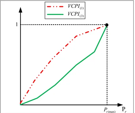
Voltage Collapse Proximity Indicator (VCPI)
Voltage collapse proximity indicators (VCPI) are based on the theory of maximum power transfer between two buses (Moghavvemi et Faruque, 1998):
( )= ( ) (1.5) ( )= ( ) (1.6)
where and are active and reactive power transferred to the receiving end. ( ) and
( ) are the maximum active and reactive power that can be transferred.
( )=
( )
(1.7)
where is active power losses in the line and ( ) is the maximum possible active power
losses. All values are calculated from the power flow calculations. The behavior of these indices is approximately linear in the cases with light loads. ( ) is more sensitive at
higher load than ( ) in the proximity to the voltage collapse point (due to ). The behavior of ( ) and ( ) is shown in Figure 1.10 when the power transfer through
the line increases gradually. These indices have several advantages such as greater accuracy, the easy calculation, and the recognition of weak lines.
Line Stability Factor
Line Stability Factor is defined as an index to monitor online the voltage evaluation based on the transmission line calculation. When the value of this factor reaches to 1.0, it shows that the system becomes unstable. This index is defined as (Mohamed, Jasmon et Yusoff, 1989):
= 4 + (1.8)
where subscripts of and shows sending and receiving buses in the considered transmission line, respectively; is the line reactance.
1
P
r (1) VCPI (3) VCPI (max) r PFigure 1.10 Comparison between voltage collapse proximity indicators Adapted from Moghavvemi and Faruque (1998)
Line Stability index is used to evaluate the system stability and when the value of reaches to 1.0, it shows that the system becomes unstable. The index equation is given as follows:
=[ 4
( − )]
(1.9)
where ∠ is the line reactance and is the angle difference between two buses. An advantage of this index is that can distinguish between weak and strong transmission lines. It also helps the ISO to find the voltage collapse in the vicinity of bifurcation point. Moreover, the computational burden is relatively low which is proper for large power system (Moghavvemi et Omar, 1998).
Fast Voltage Stability Index (FVSI)
FVSI is a criterion that shows both voltage stability situation and contingency ranking. This index is used to predict the system instability when the value of FVSI reaches to 1.0. The FVSI is defined as (Musirin et Rahman, 2002):
=4 (1.10)
The calculation process of this index like other LVSIs is based on the single transmission line calculation. Thus, they are more compatible with the contingency ranking. A disadvantage of these methods is that they cannot give any idea about the weak buses and only show the weak lines.
(Cupelli, Doig Cardet et Monti, 2012) shows a comparison between these four indices based on accuracy, control adequacy and robustness to the load increase. Generally, all indices represent the linear behavior before reach to the voltage collapse. But they show a nonlinear
behavior during the voltage collapse. The values of Lmn and LQP indices increase more than one and they detect wrongly the voltage instability. Otherwise, the results show that the VCPI is the best index from the mentioned criteria and it is less dependent on the load dispatch.
1.4.4 Indices based on L-Index
An indicator L (L-Index) is introduced as a quantitative value to calculate the distance from the operating points to the stability limit (Kessel et Glavitsch, 1986). The system admittance matrix is defined by the load and generator buses as follows:
= (1.11)
The voltages at the load buses can be shown as:
= − = + (1.12)
where = ( ) and = − .
For a particular load bus , we have
=
∈
+
∈
(1.13)
Gm
V
LL LG GL GGY
Y
Y
Y
NY
1 GV
GiV
1I
iI
mI
1 LV
LjV
LkV
1I
jI
kI
Figure 1.11 Power system model with m PV bus and k Loads (L Index) Adapted from Yang, Caisheng et al. (2013)
L index is defined as:
= 1 −∑∈ (1.14)
When the value of becomes 1.0 or close to 1.0, it shows that the voltage at bus is near to its voltage stability limit. The contingencies affect on the L-Index due to changing the system state like new voltage profile. Calculation of the L-Index is simple, time-saving and it can be changed easily. The L-index has an accurate result when the loads gradually increase.
(Salama, Saied et Abdel-Maksoud, 1999) describes a simplification method for calculation of L-Index, which reduces the computational burden. It suggests using the imaginary parts of the admittance matrix in the L-index formula. Thus, instead of using = −( ) , it is changed as follows:
where and are the imaginary parts of sub-matrices of the admittance matrix. This simplification is useful for large power systems and it can increase the calculation speed, because the matrices with only imaginary part can be inverted quickly. The comparison between with/without simplification shows that the results are very close and acceptable.
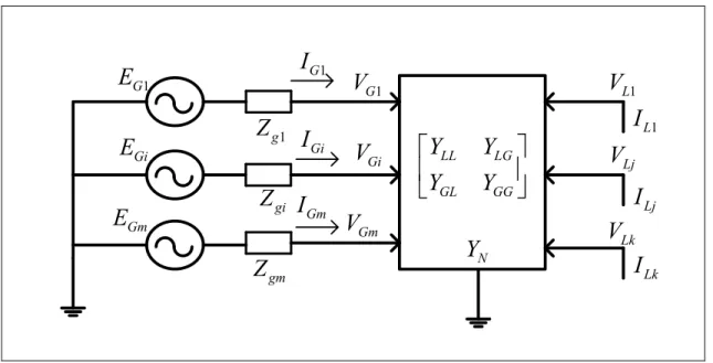
When the distance of generators and loads become closer or/and the PV generators have converted to the PQ nodes in case of the reactive power limits, the L-Index is not very accurate. (Yang et al., 2013) has proposed an extended L-Index that uses a complete generator equivalent model (GEM). This model adds an equivalent internal impedance in front of a voltage phasor . The extended L-index is obtained as follows:
= 1 −∑∈ (1.16)
In conclusion, the results shows that extended L-Index can predict better the voltage collapse than the L-Index.
Gm
V
LL LG GL GGY
Y
Y
Y
NY
1 GV
GiV
1 GI
GiI
GmI
1 LV
LjV
LkV
1 LI
LjI
LkI
GmE
1 GE
GiE
gmZ
1 gZ
giZ
Figure 1.12 Power system model with m PV bus and k Loads (Extended L Index) Adapted from Yang, Caisheng et al. (2013)