HAL Id: hal-00784336
https://hal.archives-ouvertes.fr/hal-00784336
Submitted on 5 Aug 2013
HAL is a multi-disciplinary open access
archive for the deposit and dissemination of
sci-entific research documents, whether they are
pub-lished or not. The documents may come from
teaching and research institutions in France or
abroad, or from public or private research centers.
L’archive ouverte pluridisciplinaire HAL, est
destinée au dépôt et à la diffusion de documents
scientifiques de niveau recherche, publiés ou non,
émanant des établissements d’enseignement et de
recherche français ou étrangers, des laboratoires
publics ou privés.
Proactive production activity control by online
simulation
Olivier Cardin, Pierre Castagna
To cite this version:
Olivier Cardin, Pierre Castagna. Proactive production activity control by online simulation.
Inter-national Journal of Simulation and Process Modelling, Inderscience, 2011, 6 (3), pp.177-186.
�hal-00784336�
Proactive production
activity control by online
simulation
Olivier Cardin
IRCCyN
1 rue de la Noë – BP 92 101 – 44321 Nantes Cedex 03 E-mail: [email protected]
Pierre Castagna*
IUT de Nantes, Département QLIO – IRCCyN
2 Avenue du Professeur Jean Rouxel – BP 539 – 44475 Carquefou E-mail: [email protected]
*
Corresponding authorAbstract: In this paper, we present a new application of Discrete-Event
Simulation as a forecasting tool for the decision support of the production activity control of a complex manufacturing system. The specificity of such an application of simulation is the short term of the forecasts. This specificity implies that the initial state of the simulation takes into account the actual state of the system. A development on a real-size Flexible Manufacturing System shows the technical feasibility of the developed concepts and the potential benefits on the productivity of a single example.
Keywords: Decision support, Online simulation, Real-time Simulation,
Simulation initialisation, Observer, Synchronisation.
Biographical notes: Olivier Cardin is associate professor in University of
Nantes, mechanical engineering department. He is a member of the Communication and Cybernetic Research Institute of Nantes (IRCCyN UMR CNRS 6597, France). His current research focuses on the use of discrete-event simulation as a decision support in the production activity control of complex manufacturing systems, such as product-driven ones. Pierre Castagna is a Professor of the University of Nantes, in Industrial Engineering. He is member of « Institut de Recherche en Communications et Cybernétique de Nantes » UMR CNRS 6597. After attending an initial education in mechanical engineering and automatic control, he is currently working on formalism for specification of simulation models, distributed simulation, discrete event simulation and transfer system design. He has been a scientific manager of more than 30 research contracts (with AIRBUS, TRELLEBORG, SOCCATA, etc.).
1 INTRODUCTION
As the complexity of the manufacturing systems increases, the operators in charge of the management of such systems have more and more difficulties to make the correct decisions. As a matter of fact, the decision support tools become
more and more important in the control architecture and towards the performance requirements of the system. These decision support tools are constituted of a Graphic User Interface (GUI) and forecasting features. These features are for example based on scheduling algorithms/heuristics, ant colony algorithms for a multi-criteria optimization, etc. The problems the operators have to face are mainly due to the disruptions that appear inside the
workshop. These disruptions may be either internal (machine breakdowns, operator missing, etc.) or external (supply failure, urgent fabrication orders, etc.). When they appear, the operator needs to decide of a curative action. Facing several choices, he needs an evaluation of the impact his decision might have on the future behaviour of the workshop.
(Pujo et al., 2004) defined the concept of proactive production activity control by means of simulation. These simulations aim to determine future performance indicator based on the current one in a KANBAN type production line. These indicators are analysed to detect in advance the problems that might appear in the systems in the future to try and correct it before it even happens.
Our approach is slightly different: the simulations are not launched periodically to anticipate the current behaviour of the system, but is launched on demand in order to test the impact of the operator‟s decisions on the future behaviour of the system. As a matter of fact, first part of this paper deals with the notion of online simulation, in which our work is located. Then, the relative places of human and machine are discussed, in order to define the place of the simulation tool in the decision support architecture. After the problem of the initialisation of the simulations is treated, an example of real-size application is treated in order to validate technically the approach, and to demonstrate the benefits of the tool on a simple example.
2 ONLINE SIMULATION
In the past 20 years, several work dealt, in many ways, with the concepts of proactive simulation. For example, (Wu and Wysk, 1987) choose to discretize the production time (dt). At the beginning of each dt, a simulation is launched to test several local scheduling rules and decide which one is the best according to one or several criteria (mean flow time, makespan, etc.). At this time, these rules are applied during the next dt, and the whole procedure is executed again dt later.
In 1999, (Kouiss and Pierreval, 1999) propose an application based on an online simulation. This application aims to monitor the system by the analysis and the comparison between the real and simulated data on one hand, and to help the operator to make mainly scheduling decisions on the other hand. To validate the approach, an application was developed on a real-sized FMS settled in the IFMA of Clermont-Ferrand, France.
(Hanisch et al., 2003) deal with the simulation of the evolution of the people flows in a public place (railway station, airport, shopping centre,
etc.). The goal is to create a transparent online simulation (the operator does not have to start and parameterize the simulations, nor to analyse raw simulation results) to make decisions about the regulation of the pedestrian flows in the rush hours. The prototype has to be able to anticipate and warn about overcrowding problems in the “storages” (shops, corridors, etc.) on a short term considering the actual flows. A set of simulations is launched every 5 minutes. The problem is there are almost no simulation tools in the operative phase to organise the displacement of large quantities of pedestrians in large public places.
Several characteristics radically distance online simulation from classical use of simulation (in design phase for example). One of the main is that the simulation horizon is obviously short relatively to the dynamic of the system to state about the effect of the short term decisions. Because of this, the initial state of the system in the simulation is a very influent point on the results, thus on the decision. (Davis, 1998) states that the simulation model has to be connected on-line with the real world. It means that each time a simulation starts, the model has to be initialized with the actual state of the real system. The second characteristic is that the simulation results have to be available before a deadline, the system evolving between the beginning of the simulations and the display of the results. The simulation engine has to be powerful enough to deliver the results in a short lap of time so that they may be used in the decision process. The simulation models which fulfil these conditions are classified by (Davis, 1998) as being models of “online simulation”.
3 HUMAN-MACHINE COOPERATION IN DYNAMIC SITUATIONS
3.1 State of the art
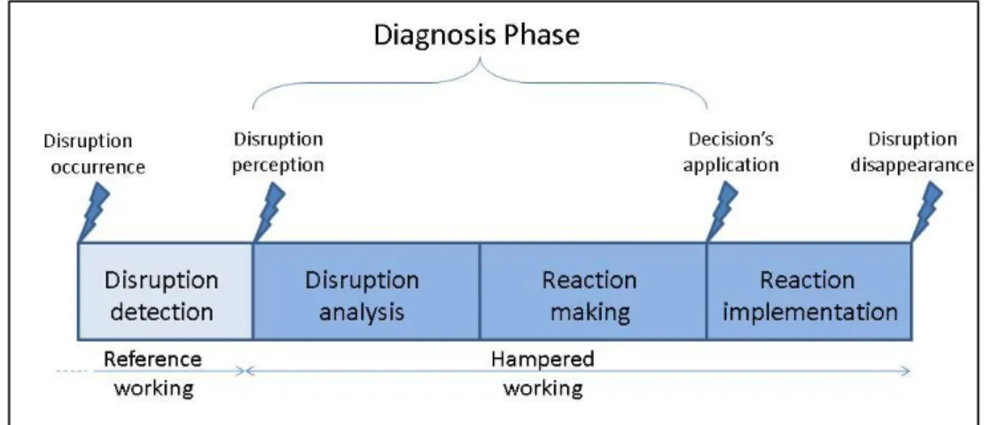
Since the early 1980‟s, humans roles are moving from operating to monitoring and decision tasks. Problems are now about the decision support for production activity control or production management, for monitoring, diagnosis or reconfiguration of the facility in case of disruption. In (Cauvin, 2005), Cauvin defines a disruption as an unscheduled event likely to hamper the production process and sometimes to jeopardise the objectives of the production. These disruptions may mainly occur on five aspects of the production system:
- Availability of internal resources (unavailability of machines, etc.);
- Demand (surprising success of a product, etc.);
- Information (data transcription mistakes, etc.);
- Decision (data mistaken into account, etc.). The author also describes the life cycle of such a disruption (Figure 1).
Figure 1 The disruption’s life cycle From the perception of the disruption, the
human has to elaborate a diagnosis. The definition taken here was presented in (Hoc, 1990) and (Cegarra and Hoc, 2001): “a comprehension activity relevant to an action decision”. The authors say that “diagnosis is an activity of comprehension, organising elements into a meaningful structure. This organisation is oriented by the operator towards decisions relevant to actions. While diagnosing, the operator manages a balance between benefits and costs, trying to reach an acceptable performance according to the goals.”During the diagnosis phase described in (Cauvin, 2005), the operator has to analyse (identify and characterise) the disruption and to determine how to react.
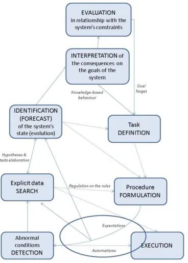
(Hoc, 1996) presents a revised version of Rasmussen‟s model (Rasmussen, 1983) (Rasmussen, 1986) of human approach for problem solving in the diagnosis phase (Figure 2). As soon as the operator has detected the disruption, he evaluates the situation by observing available data (Disruption analysis) and identifies and/or forecasts the state of the system. Then, he makes up a solution taking into account constraints and risks (Reaction making).
Hoc‟s revisions modify Rasmussen‟s initial model by adding the cognitive mechanisms of situation evaluation: diagnosis and/or forecast by a method based on hypotheses elaboration and tests. In this model, the operator is considered as a problem solver, but the question is to know how far the machine may help the operator in this task.
A lot of decision support systems were developed in the past (e.g. based on planning heuristics, etc.): these systems make sense in the
FORECAST phase. Indeed, the operator needs to know the impact of each decision he could make on the future behaviour of the system to be able to choose correctly. As a matter of fact, he needs a forecasting tool.
When considering production systems which do not have any satisfying analytical modelling of its behaviour, or any powerful algorithms or heuristics developed, discrete-event simulation is a powerful and well-dedicated tool to use. As it is possible to model complex processes with a great level of detail, a trial-and-error methodology is very well-adapted.
This is why we think it is relevant to try and give the opportunity to use simulation in the online short-term decision making process.
The first question we will try to answer is to determine at which level of automation the system has to be. Endsley and Kaber (1999) proposed a hierarchy of levels of automation applicable to dynamic-cognitive and psychomotor control task performance (Table 1). As stated before, the diagnosis phase deals with the “Generating” and “Selecting” tasks.
A first approach would be to have a “Full Automation”. This is well dedicated to very well known disrupts, where all the procedure are very well established.
In most cases, the detection and analysis of disrupts cannot be fully automated. Monitoring is thus dedicated to Human with Computer; on the other hand, Implementing is in most cases dedicated to Computer. A second approach would be to have a “Rigid System”, where computer makes up all the hypotheses and runs the tests automatically. Then, it presents the decisions to
human for approval. In (Hoc, 2001), the author points out four main types of difficulties between human and automation: one of them is called “Complacency”. It is said that, even if the operator knows from his expertise a better solution, he may
adopt the computer‟s proposals. It is thus recommended that the machine proposes several solutions instead of a single one to encourage mutual control.
Figure 2 Problem solving model ((Rasmussen, 1983, 1986) revised by (Hoc, 1996))
Roles (
Level of automation Monitoring Generating Selecting Implementing
Manual Control H H H H
Action Support H/C H H H/C
Batch Processing H/C H H C
Shared Control H/C H/C H H/C Decision Support H/C H/C H C Blended Decision Making H/C H/C H/C C
Rigid System H/C C H C
Automated Decision Making H/C H/C C C Supervisory Control H/C C C C
Full Automation C C C C
Table 1 Hierarchy of levels of automation applicable to dynamic-cognitive and psychomotor control task performance (Endsley and Kaber, 1999)
To encourage the pilot to be an actor of the decision making, we may finally consider a “Decision Support”, where Human and/or
Computer make up the hypotheses as Computer runs the tests and display the numbered results, up to the Human alone to make the decision.
This paper focuses on the description of the insertion of online simulation in the “Decision Support” level of automation. However, several prototypes of the other modes were made, and the results are comparable with those presented here.
3.2 Integration in the decision making process
In a global way, simulation based decision making corresponds to an experimental methodology. Making a decision is selecting values of a set of parameters being the entrance vector of the system. A set of simulations is run and at the end of each, the operator analyses the results to determine whether he shall run another simulation after adjusting the entrance vector or if, the results being satisfying enough, the entrance vector is considered as the best solution and thus the decision to take. A major drawback of this methodology is of course the time needed to reach the best solution (or at least a satisfying one). This is a crucial point when talking about online simulation, where decision has to be made and applied in a very short time. Furthermore, as the state of the system has a great influence on the results and has changed during the decision making process, this evolution has to be taken into account. Therefore, the operator has to evaluate the total duration of the decision making process as a first step.
The decision making process can be described in the following 5 steps:
(1) Choice by the operator of the appropriate model, according to the type of decision he has to make. This model is chosen in a pre-established models library, as the short delays prevent operators to build the model at the time of the decision. Let us note the duration of this step.
(2) Determination of the factorial experiment leading to test hypotheses. (Duration : )
(3) Retrieving the actual state of the system to initialise simulations (see following section of this paper for further details). (Duration: )
(4) Running the simulations corresponding to hypotheses. If the simulation model is stochastic, each hypotheses lead to replications to build a satisfying confidence interval enabling the decision to be made (each replication has a duration).
(5) Analysing the results. (Duration: ) Therefore, we can write the total duration of the methodology:
Step (3) is automated, thus is very small. Steps (1), (2) and (4) have to be rigorously prepared to reduce duration D without shortening step (5) too much. In a stochastic analysis, step (4) may have the longest duration, thus the operator will have to be very careful about the value of the
product. The advantage of such a break down is that the separate durations are relatively constant according to the model. When the operator has chosen the appropriate model (step (1)), it is possible to retrieve the average durations obtained of the previous use of that model to approximate the effective durations of the actual case. As a matter of fact, a minor decision support for the operator to determine the duration according to the product shall be integrated in the user interface.
4 INITIALISING A ONLINE SIMULATION
As stated before (step (3)), the retrieval of the actual state of the system is very important in order to correctly initialise the simulations.
4.1 Problematic
(Hanisch et al., 2005) explain that, in the classical simulation approach, the models are initialized in an “empty” and “idle” state. An initial bias is sometimes needed to adjust the statistics, but that is often enough to ensure the validity of the results. In online simulation, that cannot be the case, because it seems hard to archive the trace of several thousands of hours of working in a sufficiently precise way not to influence to much the bias. The model has to be parameterised directly from data obtained at the actual moment on the real system. In a simple case, the state of the objects of the simulation model may directly be identified through measurements performed on the field. The accuracy and availability of the data conditions is not guaranteed for every application, even if the models initialisation methods presented in the literature always need them to be generalised.
As a matter of fact, (Fowler and Rose, 2004) state that, for any tool to be able to reproduce the actual state of a real system (in their case a FMS), the following problems have first to be solved:
- A clear and accurate definition of the expression “actual state of the system” is missing:
before starting to collect data, we need to know precisely what type of data we have to collect to obtain an accurate image of the system;
- There is a lack of data: needed data for the
simulation are not always available or cannot be automatically deduced from other data on the system;
- The data quality is too low: for example,
the simulation model needs an histogram can only provide mean values of one of the parameters;
- The data update frequency is too low: for
dates after an often relatively long delay, let‟s say once a day.
To solve all these problems, we propose to use a real-time simulation as an observer of the system. This simulation will be used to compute in real-time the initial bias from the data retrieved from the real system, and when an online simulation needs to be launched, the actual state of the simulation is used as a good approximation of the state of the system.
4.2 Accuracy of the observer
As the state of the observer is only an approximation of the real system‟s state, it has to be as accurate as possible to deliver some good pieces of information. The main problem here is the modelling of the real system. Indeed, the model is meant to run for thousands of hours, and shall not deflect from reality.
In (Roy, 1989), the author extracts four sources of inaccurate determination, uncertainty and imprecision in decision models:
1. The map is not the territory: omissions, simplifications, aggregations of heterogeneous features;
2. The future is not a present to come: the future, almost always, conceals something unpredictable or indeterminable;
3. Decision application conditions: they might be influenced by the state of the environment at the time of the application if it is punctual, or during the successive steps if the decision has a sequential characteristic;
4. Highly subjective characteristics of some aspects.
In order to avoid these problems, we chose to synchronise as often as possible the observer with the real world. The communication mean used here can be of several kinds, one is described in detail in the last section of this paper.
4.3 The real-time observer
The state of the physical system is perceived through a finite number of sensors. Thus, the system‟s state can be represented as a vector V:
This means the observation model must be aware of all the situations where a synchronisation has to be performed. The change of state of each of these sensors (synchronisation points) corresponds
to an event that made the physical system evolve. These events occur at dates , with the corresponding number of the sensor and the number of the event (as several events may occur concerning the same sensor, we need to differentiate them). Between and , the observer uses local prevision functions , defined on the interval . This prevision function may be a linear relation between speed and distance to travel for example.
To sum up, we can write that:
4.4 The synchronisation with the real system
For each component , changes on date : that is the synchronisation operation. Two cases may occur.
First case corresponds to the observer being ahead of the physical system. In this case, the simulator has to wait for the real event. The model evolves until reaching such a situation, and locally waits for the corresponding event. The evolution of this part of the model will only keep going when the data arrives, whereas the rest of the model keeps on going normally.
But the opposite case may also occur: the observer being late, it receives the real event whereas the simulation did not reach the synchronisation point. We propose then a local acceleration of time in order to bring the observer in a state in keeping with the real system‟s state. This acceleration corresponds to a modification of the prevision function used by the observer to estimate the system‟s evolution between two synchronisation points.
To illustrate this, let‟s take the example of a conveyor and two sensors s1 and s2 presented in
figure 3. When parcel n°1 is in front of simulated sensor s1, the real parcel is not yet in s1: the
observer is ahead of reality. The observer then blocks parcel n°1 until real sensor s1 detects real
parcel n°1.
On the opposite, real parcel n°2 is already facing s2, when the observer considers parcel n°2 is
still approaching this sensor: the observer is late. Synchronisation will instantly place parcel n°2 in position (2b). Then, each time a piece of information about the system‟s state is known by the observer, it is synchronised. However, between
s1 and s2, the parcel‟s position is unknown. The
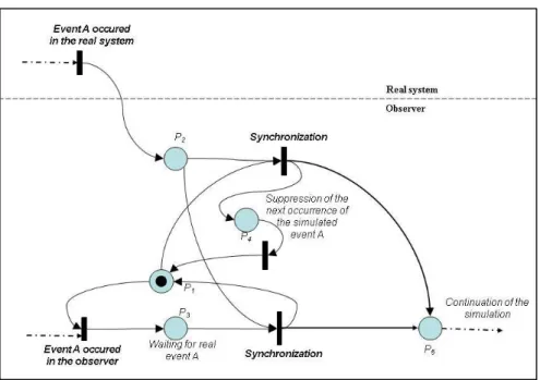
observer may be used in order to evaluate their position, thanks to the prevision functions. The synchronisation function of the observer may be formalised by the Petri Net presented figure 4. When a token is in P2, it means the event named A
happened on the real system: two transitions are linked to the place. However, they cannot be fired simultaneously, as there has to be a token in P1 or
P3, corresponding to the possibility that event A
already happened in the observer. If the token is in P3 (real A happened), synchronisation is kind of
natural and the token goes in P5. If the token is in P1
(real A did not), then the token goes in P4 and P5.
Place P4 has a particular function enabling the
observer to delete the next occurrence of the event
and to make the observer consider that this
occurrence actually happened. The token goes next in P1 to enable the wait for a new event.
Figure 3 Synchronisation example
Figure 4 The observer synchronisation function principles
5 VALIDATION ON AN EXPERIMENTAL DEVICE
5.1 The experimental device
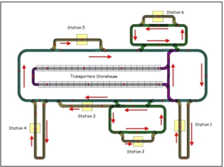
To validate this approach, we used a real-size Flexible Manufacturing System (six stations job-shop with automated transfer presented figure 5). This FMS is a good example of product-driven production (Wong et al., 2002), as the transporters have an electronic tag. A product-driven production is a typical application of our decision support device. Indeed, the transporters travel around the system interacting with their environment, the control being totally reactive. The working of such
a system consists in giving a piece of information to the tag (here the recipe of the product it has to carry) at the beginning of the production (here at the exit of the storehouse). Then, the transporters go from station to station, asking them whether they are able to perform the next requested operation of the recipe. If they are, the transporter may decide to enter the station. These decision rules are relatively simple, but only focus on a very local point of view. As a matter of fact, the global behaviour of the system is very difficult to obtain when needed. That is the case when an operator has to make a decision that might influence the whole system on a short term: for example the parameterisation of a new fabrication order.
Figure 5 The assembly line
5.1.1 The real-time observer
The aim of the observer is to represent as closely as possible the behaviour of the real system. As a matter of fact, local decision rules programmed in the PLC are faithfully reproduced in the observer programming to ensure a sufficient coherence. In the same way, system‟s physical constraints (only one transporter in each turn for example) are kept (thanks here to a resource sharing). Finally, dynamic characteristics are evaluated as correctly as possible (conveyors speed, slowing down in each turn, etc.) (Roy, 1989).
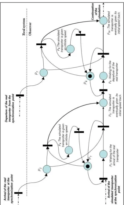
Figure 6 shows how we applied figure 4‟s Petri Net to our device when synchronising in front of a tag reader. That Petri Net is a juxtaposition of two of the event handling models presented before, as we take into account here the arrival and the departure of the transporter in front of the reader (as it might stay an unknown time in front of it, when the operation is performed by a human operator for example). Both of these events are represented in the “Real system” part of the figure.
This model‟s main adaptation considering the generic one deals with places P4 and P9. This model
proposes to infinitely accelerate the simulated transporter when it is late, and to give its initial speed back just after. Another possibility, performed on another simulation piece of software, was to delete the transporter from the observer and
to re-create another one right in front of the reader. These two possibilities are strictly equivalent in the user‟s point of view.
When the simulated transporter is ahead of the real one, it is simply stopped at the station until the real one reaches it.
5.1.2 The control architecture
Concerning the adopted architecture, the observer has to be constantly connected with two elements:
- The OPC server: it sends an event each time a pre-defined group of variables changes its value. Thus, we only need to declare a group of variables characterising the presence of a transporter in front of a sensor and to wait the evolution of this group. When that event occurs, the observer treats the embedded data (sensor‟s reference, transporter‟s number, etc.) as previously defined. This is mainly used for the synchronisation;
- The database: it stores all the system‟s production data, which are mainly needed to set the online simulations up.
Figure 7 shows how simulation is inserted in the considered control architecture of the system. This is a classical hierarchical architecture. The case of distributed control was examined in (Cardin and Castagna, 2009) through the example of Holonic Manufacturing System.
Figure 6 Adaptation of the synchronisation model
5.2 Example of online simulation in a “Decision Support” architecture
This section presents an experiment which aims to:
1. Demonstrate the benefits of online simulation on the production activity control of a complex manufacturing system;
2. Illustrate the human-machine cooperation in a “Decision Support” based architecture enabling online simulation.
5.2.1 Experimental conditions
The studied system is an emulation of the previously presented system. We chose to use an emulation of the real system in order to have reasonable experimental duration, but the behaviour and the performance of both the emulation and the real system are strictly identical. Products transporters can move on the central loop where they can enter the different stations to keep on the recipe of the product. When several products are assigned to a transporter, it treats them successively: the first operation of the recipe is typically the loading of a product on the transporter, the last is its unloading, and it loops until the last product is finished. When all of them are, the transporter goes back to the storehouse. It is only at the exit of this storehouse that the transporter may have a new mission assigned. Each mission is parameterised with:
1. The number of products to transport; 2. The recipe of the products, which is an ordered list of operations to perform (Mc Farlane, 3R);
3. The production order they correspond to. Each production order is characterised by a total number of products to make and a recipe associated.
5.2.2 Problematic
When a new order is placed, the production pilot has to decide how many transporters he allocates to the order (the total number of goods of the order is the product of the number of transporters and the number of products each transporter has to carry). If the pilot chooses a large number, it raises the traffic on the automated transfer system, which causes slow down and thus raises the makespan, when a too small number prevents the operations to be performed in parallel on several stations, and thus raises also the makespan. The pilot needs to find a compromise, which depends on:
- The recipes of the orders actually running (recipes making the products go on separate stations do not get in each other way and thus do not really have an impact on the makespan);
- The actual and the near future traffic on the job-shop (if the running production orders are close to the end or at their very beginning, the influences will not be the same);
- The number of transporters available in the storehouse.
These criteria are generally complex to analyse, as it requires a multi-criteria analysis on a relatively large amount of data. Furthermore, the short-term evolution of the system might greatly modify the values of some data.
5.2.3 Experiment’s procedure
Production starts with an empty and idle job-shop. To load it, a dummy production order is placed. Its parameters (recipe, number of products
Np) are random, except for the number of
transporters Nt which is taken equal to the number
of products (i.e. each transporter carries out one product). Parameters of the job-shop are also randomised at the beginning of the production (production times, operation repartition over the stations, etc.). When 25% of the transporters are back at the storehouse, a second order is placed. We chose 25% in order to have a line more or less loaded according to the randomisation.
In the same way, the first two parameters of the second order are randomised, but the number of transporters is left empty in order to study the impact of its value on the behaviour of the production. The experiment runs in two steps:
1. The pilot has a simple rule to apply: he chooses half of the number of transporters left in the storehouse Ns as number of transporters
allocated to the order. Of course, if this number is greater than the number of products to make, he chooses the number of products. As a matter of fact, the rule can be sum up by the formula:
The value recorded is the total production time for both of the orders;
2. The computer runs several tests in order to determine the optimum. These tests were made on 20 hypotheses, corresponding to:
with and
N the number of the hypothesis to test.
As previously, the total makespan is recorded for each test. We look for N giving the lowest makespan, and we compare this makespan
to the value obtained previously:
This experiment was driven 100 times, and all the parameters were randomised between each experiment. This repetition enables to eliminate the influence of recipes or operatory conditions on the final result. Indeed, only a slight change between two tests in the recipe for example might change completely all the results. As a matter of fact, we perform a lot of tests in order to be sure all the combinations will be evaluated.
5.2.4 Results
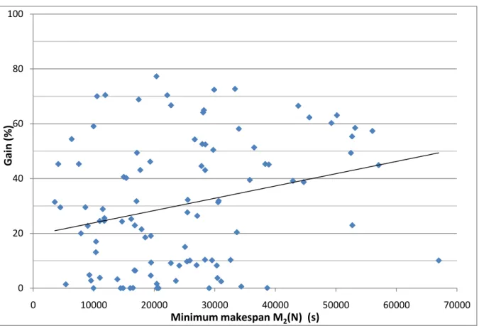
Comparing the two algorithms (figure 8 shows the gain obtained according to the makespan of the whole production), a first conclusion is that the second procedure never gives a worse result than the simple algorithm. Furthermore, the linear regression line drawn on figure 7 shows that the
gain is more important when the productions are long. This is explained by the fact that when the production time is low, the dummy order has a bigger influence on the final result, and thus the benefits of online simulation are withdrawn.
There are cases where the simple rule gives the same result as online simulation (Gain=0%), but considering the whole experiment leads to an average benefit of 30%, with a maximum around 80%. On each case, the time needed to test the 20 hypotheses and display the result(s) is less than 5 seconds. The architecture we propose is a GUI where the operator enters the parameters of the order and press a “Compute” button that starts the simulations. A first table shows all the hypotheses (pre-computed) that the computer thinks testing, table that may be modified by the pilot according to his expertise. When the simulations end up, a table showing all the tests classified in growing order of makespan is displayed and let the pilot decide. When the decision is validated, the computer implements the decision by launching the order with the chosen parameters.
Figure 8 Gain according to the whole production makespan
0 20 40 60 80 100 0 10000 20000 30000 40000 50000 60000 70000
G
ai
n
(
%)
Minimum makespan M
2(N) (s)
6 CONCLUSION
This paper deals with the use of online simulation in the production activity control of a complex manufacturing system. After defining which were the respective places of human and machine in the architecture, this paper gives solutions in order to avoid the initialisation of the simulation problems. This solution is based on the use of a real-time simulation as an observer of the actual behaviour of the system. The state of this observer is used as the best approximation of the real state for the initial state of the online simulations. Finally, we treated an example of application, which demonstrates the technical feasibility of the solution and gives an idea of the benefits the use of the tool can give on a single example.
This example was based on the “Decision Support” level of automation. As stated before, a “Rigid System” level, or even a “Full automation” can be considered. This last level was already presented in (Cardin and Castagna, 2006). This example deals with the use of online simulation directly from the Programmable Logic Controllers (PLC) in the priority rule of a machine supply.
The actual works on this subject focus on the temporal evaluation of this solution: does the approximation made by the use of the observer have a great influence on the final result? What are the communication delays between the occurrence of an event in the real world, and its application in the observer?
REFERENCES
Cardin, O. and Castagna, P. (2006) „Handling uncertainty in Production Activity Control using proactive simulation‟, in Proceedings of 12th
IFAC Symposium on Information Control Problems in Manufacturing. INCOM,
Saint-Etienne, France, pp. 579-584
Cardin, O. and Castagna, P. (2009) „Using online simulation in Holonic Manufacturing Systems‟,
Engineering Applications of Artificial Intelligence, vol. 22, pp.1025-1033.
Cegarra, J. and Hoc, J. M. (2006) „Cognitive styles as an explanation of expert‟s individual differences: A case study in computer-assisted troubleshooting diagnosis‟, International Journal of Human-Computer Studies, Vol. 64,
pp. 123-136.
Cauvin, A. (2005) Analyse, modélisation et
amélioration de la réactivite des systèmes de décision dans les organisations industrielles:
vers une aide à la conduite des processus d'entreprise dans un contexte perturbé,
Habilitation à diriger les recherches, Université Paul Cézanne, Aix-Marseille III.
Davis, W. J. (1998) „On-line simulation :Need and evolving research requirements‟, in J. Banks (Ed) Handbook of Simulation, New York, John Wiley and Sons Inc., pp. 465-516, ISBN 0-471-13403-1.
Endsley, M. R. and Kaber, D. B. (1999) „Level of automation effects on performance, situation awareness and workload in dynamic control task‟ Ergonomics, Vol. 42, No. 3, pp. 462-492. Fowler, J. W. and Rose, O. (2004) „Grand
challenges in modelling and simulation of complex manufacturing systems‟, Simulation, Vol. 80, pp. 469-476.
Hanisch, A., Tolujew, J., Richter, K. and Schulze, T. (2003) „Online simulation of pedestrian flow in public buildings‟, in S.Chick, P.J. Sánchez, D. Ferrin, and D.J. Morrice (Eds) Proceedings
of the 2003 Winter Simulation Conference,
Piscataway, pp. 1635-1641
Hanisch, A., Tolujew, J. and Schulze, T. (2005) „Initialization of online simulation models‟, in M.E. Kuhl, N.M. Steiger, F.B. Armstrong, and J.A. Joines (Eds) Proceedings of the 2005
Winter simulation conference, pp. 1795-1803.
Hoc, J.M. (1990). „Les activités de diagnostic‟, In J.F. Richard, C. Bonnet, & R. Ghiglione (Eds.),
Traité de psychologie cognitive. Tome II: Le traitement de l'information symbolique. Paris:
Dunod, pp. 158-165.
Hoc, J.M. (1996) Supervision et contrôle de
processus, la cognition en situation dynamique,
Presses Universitaires de Grenoble.
Hoc, J.M. (2001) „Towards a cognitive approach to human-machine cooperation in dynamic situations‟, International Journal of
Human-Computer Studies, Vol. 54, pp. 509-540.
Kouiss, K. and Pierreval, P. (1999) „Implementing an on-line simulation in a flexible manufacturing system‟, in Proceedings of the
ESS'99 Conference, Nuremberg, Germany,
26-28 October 1999, pp. 484-488.
McFarlane, D., Carr, J., Harrison, M. and McDonald, A.(2002) Auto-ID's three R's: Rules
and Recipes for product Requirements, Auto-ID
Center White paper.
Rasmussen, J. (1983) „Skills, rules and knowledge; Signals, signs and symbols and other distinctions in human performance models‟
IEEE SMC, No. 3.
Rasmussen, J. (1986) „Information processing and human-machine interaction; An approach to cognitive engineering‟, in P. Sage (Ed) System
Roy, B. (1989) „Main sources of inaccurate determination, uncertainty and imprecision in decision models‟, Mathematical Computer
Modelling, Vol.12, No. 10/11, pp. 1245-1254.
Wong, C.Y., McFarlane, D., Zaharudin, A. and Agarawal, V. (2002) „The Intelligent Product Driven Supply Chain‟, in Proceedings of IEEE
Systems Man and Cybernetics, Hammammet,
Tunisia.
Wu, S-Y. D. and Wysk, R. A. (1989) „An application of discrete-event simulation to on-line control and scheduling in flexible manufacturing‟, International Journal of
Production Research, Vol. 27, No. 9, pp.