Climate change damages to Alaska public infrastructure and the economics of proactive adaptation

Climate change damages to Alaska public infrastructure

and the economics of proactive adaptation

The MIT Faculty has made this article openly available.

Please share

how this access benefits you. Your story matters.

Citation

Melvin, April M. et al. “Climate Change Damages to Alaska Public

Infrastructure and the Economics of Proactive Adaptation.”

Proceedings of the National Academy of Sciences 114, 2 (Janaury

2017): E122–E131 © 2017 National Academy of Sciences

As Published

http://dx.doi.org/10.1073/pnas.1611056113

Publisher

National Academy of Sciences (U.S.)

Version

Final published version

Citable link

http://hdl.handle.net/1721.1/111200

Terms of Use

Article is made available in accordance with the publisher's

policy and may be subject to US copyright law. Please refer to the

publisher's site for terms of use.

Climate change damages to Alaska public

infrastructure and the economics of

proactive adaptation

April M. Melvina_{, Peter Larsen}b_{, Brent Boehlert}c,d_{, James E. Neumann}c_{, Paul Chinowsky}e_{, Xavier Espinet}e_,

Jeremy Martinichf,1, Matthew S. Baumannc, Lisa Rennelsc, Alexandra Bothnerc, Dmitry J. Nicolskyg, and Sergey S. Marchenkog

a_{American Association for the Advancement of Science (AAAS) Science & Technology Policy Fellow, Climate Change Division, US Environmental Protection}

Agency, Washington, DC 20460;b_{Independent Consultant, Helena, MT 59601;}c_{Industrial Economics, Inc., Cambridge, MA 02140;}d_{Joint Program on the}

Science and Policy of Global Change, Massachusetts Institute of Technology, Cambridge, MA 02139;e_{Resilient Analytics, Boulder, CO 80309;}f_Climate

Change Division, US Environmental Protection Agency, Washington, DC 20460; andg_{Geophysical Institute, University of Alaska, Fairbanks, AK 99775}

Edited by B. L. Turner, Arizona State University, Tempe, AZ, and approved November 9, 2016 (received for review July 7, 2016)

Climate change in the circumpolar region is causing dramatic environmental change that is increasing the vulnerability of in-frastructure. We quantified the economic impacts of climate change on Alaska public infrastructure under relatively high and low climate forcing scenarios [representative concentration pathway 8.5 (RCP8.5) and RCP4.5] using an infrastructure model modified to account for unique climate impacts at northern latitudes, including near-surface permafrost thaw. Additionally, we evaluated how proactive adaptation influenced economic impacts on select in-frastructure types and developed first-order estimates of potential land losses associated with coastal erosion and lengthening of the coastal ice-free season for 12 communities. Cumulative estimated expenses from climate-related damage to infrastructure without adaptation measures (hereafter damages) from 2015 to 2099 totaled $5.5 billion (2015 dollars, 3% discount) for RCP8.5 and $4.2 billion for RCP4.5, suggesting that reducing greenhouse gas emissions could lessen damages by $1.3 billion this century. The distribution of damages varied across the state, with the largest damages projected for the interior and southcentral Alaska. The largest source of damages was road flooding caused by increased precipitation followed by damages to buildings associated with near-surface permafrost thaw. Smaller damages were observed for airports, railroads, and pipelines. Proactive adaptation reduced total projected cumulative expenditures to $2.9 billion for RCP8.5 and $2.3 billion for RCP4.5. For road flooding, adaptation provided an annual savings of 80–100% across four study eras. For nearly all infrastructure types and time periods evaluated, damages and ad-aptation costs were larger for RCP8.5 than RCP4.5. Estimated coastal erosion losses were also larger for RCP8.5.

Alaska

|

climate change

|

damages

|

adaptation

|

infrastructure

C

limate change at high latitudes is causing rapid and un-precedented environmental change. The rate of temperature rise across the Arctic has been twice the global average in recent decades (1–3). Sea and land ice has diminished (4, 5), and in-creased coastal erosion (6, 7), permafrost thaw (8–10), and wildfire activity (11–14) have been observed. Models project that these changes will continue (15–17) and that the corresponding societal impacts will be greater (18) without substantial near-term global reductions in greenhouse gas (GHG) emissions. In the state of Alaska and across the broader circumpolar north, these changes are exacerbating existing challenges and in-troducing new risks for communities, including increased dam-age to critical infrastructure (19–21).

Climate change increases the vulnerability of infrastructure by enhancing environmental stressors, thereby creating additional strains on structures beyond what is expected from normal conditions and use. Risks to infrastructure associated with cli-mate change in the Arctic have been studied previously for some

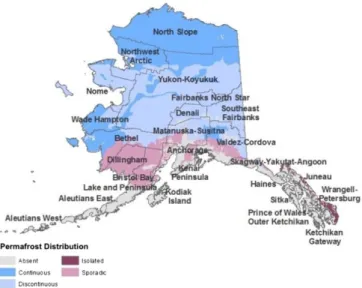
environmental stressors. Increased near-surface permafrost thaw associated with climate warming has been widely recognized as a cause of increased infrastructure damage (22–25). This climate-driven thaw can occur concurrent with thaw induced by natural disturbances, such as wildfire (26, 27), and human activities (20, 23, 27, 28), including the construction of infrastructure. Perma-frost thaw and subsequent ground subsidence, particularly where permafrost is ice-rich, negatively impact buildings, roads, rail-roads, pipelines, and oil and gas infrastructure (19, 20, 24, 29). In Alaska, Hong et al. (25) found the greatest near-term risks of thaw settlement in relatively warm permafrost found in the dis-continuous permafrost zone in the interior and longer-term risks in the continuous permafrost zone in the northern part of the state (Fig. 1 shows a map of permafrost distribution). Warmer temperatures can also alter the frequency of freeze–thaw cycles (FTCs), impacting foundation and underground infrastructure stability and vulnerability (30, 31). Extensive erosion influenced by sea ice loss, permafrost thaw, and inland flooding (7, 32) threatens numerous coastal and riverine communities in Alaska and affects most infrastructure types (33). As climate change continues, the extent of infrastructure damage as well as the costs

Significance

Climate change in Alaska is causing widespread environmental change that is damaging critical infrastructure. As climate change continues, infrastructure may become more vulnerable to damage, increasing risks to residents and resulting in large economic impacts. We quantified the potential economic damages to Alaska public infrastructure resulting from climate-driven changes in flooding, precipitation, near-surface perma-frost thaw, and freeze–thaw cycles using high and low future climate scenarios. Additionally, we estimated coastal erosion losses for villages known to be at risk. Our findings suggest that the largest climate damages will result from flooding of roads followed by substantial near-surface permafrost thaw-related damage to buildings. Proactive adaptation efforts as well as global action to reduce greenhouse gas emissions could considerably reduce these damages.

Author contributions: A.M.M., B.B., and J.M. developed and coordinated the study; P.L. contributed to study development and provided expert guidance; B.B., J.E.N., P.C., X.E., M.S.B., L.R., A.B., D.J.N., and S.S.M. compiled data and performed the technical analyses; and A.M.M. wrote the paper, with input on technical methods from all authors. The authors declare no conflict of interest.

This article is a PNAS Direct Submission.

Freely available online through the PNAS open access option.

1_{To whom correspondence should be addressed. Email: martinich.jeremy@epa.gov.} This article contains supporting information online atwww.pnas.org/lookup/suppl/doi:10. 1073/pnas.1611056113/-/DCSupplemental.

to maintain, replace, and adapt the built environment are expec-ted to increase.

Few studies have moved beyond observation and risk evalua-tion to quantify the potential economic impacts of climate change on Alaska public infrastructure. Climate change-related increases in costs have been estimated at about $50 million (original values converted to 2015 dollars using the Consumer Price Index) annually (34) for a subset of stressors affecting roads and the electricity sector, whereas Larsen et al. (35) esti-mated approximately $7.3–14.5 billion (from 2006 to 2080; val-ues converted to 2015 dollars using the Consumer Price Index) above “normal” operations and maintenance resulting from permafrost thaw, flooding, and coastal erosion impacts on a wide range of infrastructure types. In recent years, the analysis by Larsen et al. (35) has served as a guide for considering damage to infrastructure in Alaska and the broader Arctic under different climate futures. Although this study has provided valuable insights, the authors noted that estimates could be improved considerably with a more comprehensive inventory of public infrastructure and the use of nonlinear damage functions that better capture rela-tionships among environmental stressors, infrastructure lifespan, and the associated incremental change in capital and operation and maintenance costs (35, 36).

We addressed the recommendations made by Larsen et al. (35) and developed new estimates of potential economic impacts of climate change to Alaska’s public road, building, airport, rail, and pipeline infrastructure. Using high and low climate forcing scenarios [representative concentration pathway 8.5 (RCP8.5) and RCP4.5, respectively, from the Coupled Model Intercom-parison Project Phase 5 (CMIP5)] (37) for five general circula-tion models (GCMs), we evaluated the climate-related change in incurred costs (hereafter damages) required to maintain in-frastructure. We estimated the benefits (or avoided damages) to infrastructure of global reductions in GHG emissions and iden-tified where proactive adaptation measures may reduce climate change-related expenses. Climate model projections were in-corporated into a reconfigured version of the Infrastructure Planning Support System (IPSS) software tool (38–40) that ac-counts for climate change impacts unique to northern latitudes, including near-surface permafrost thaw and extreme freeze–thaw dynamics. This model also considers damages from precipitation

and precipitation-caused flooding. Independently, we developed an approach to generate first-order estimates of projected coastal erosion rates and evaluated how GHG mitigation may influence erosion in 12 coastal communities where immediate actions to manage erosion or relocate have been recommended (33). This study is one component of a broader multisector modeling framework developed for the Environmental Protection Agency Climate Change Impacts and Risk Analysis Project (41, 42), which seeks to quantify the avoided or reduced impacts of cli-mate change resulting from GHG mitigation and adaptation.

Results

Damages.The analysis presented here was designed to isolate the incremental change in damages and expenditures resulting from climate change. Costs incurred as a result of operation and maintenance or infrastructure replacement required irrespective of climate change are not included in the damage values. For precipitation, flooding, and freeze–thaw stressors, damages represent the expenditures required to maintain current levels of service, enabling the infrastructure to remain functional through the intended design lifespan. In the case of near-surface per-mafrost thaw, where repair approaches are limited, damages represent the cost of infrastructure replacement. Damage esti-mates reflect expenditures incurred when no adaptation mea-sures are taken. Adaptation costs are quantified separately and explained in Adaptation. Reported damages (and adaptation costs) reflect the difference between projected values and a historic baseline period (1986–2005) (detailed in Methods andSI Text) to isolate climate change impacts from weather variability not attributed to climate change. When the IPSS determines that infrastructure is in need of replacement, the model tabulates expenditures based on historical building standards and con-struction costs. Therefore, the damage estimates do not estimate the effect that more climate-resilient construction could provide or additional design and engineering costs associated with such efforts. Although this estimation approach may not seem intuitive, in practice, it is generally the construction approach taken, be-cause design and construction practices follow established codes and guidelines. The specific types of damages modeled in the IPSS are summarized in Table 1 and detailed inMethods.

We used two approaches to present damages (and adaptation costs) in this study: cumulative estimates for the 2015–2099 time period reported in 2015 dollars and discounted at 3% and annual undiscounted estimates that represent expenditures across four 20-y eras. The discounted cumulative values reflect the net value in the present day, thereby providing an equal basis to sum and compare the values for different time periods. A 3% discount rate is commonly used in climate impacts literature and consis-tent with the central rate used in the US Government’s Social Cost of Carbon estimates (43). For reference, we have provided cumulative undiscounted values inTable S1but do not discuss them here. We present undiscounted mean annual damages and adaptation costs across study eras to illustrate the trajectory of impacts between the two RCPs over time, which can be masked when discounting is applied (i.e., late century differences be-tween RCPs can be minimized after discounting).

Statewide Damages to Infrastructure. Total cumulative (dis-counted) damages to infrastructure (without adaptation) result-ing from projected climate change this century were estimated to be approximately $5.5 billion for RCP8.5 and $4.2 billion for RCP4.5 (Table 2). For both RCPs, flooding associated with changes in precipitation accounted for about 45% of damages, and near-surface permafrost thaw was responsible for 38% (although high variability was observed among GCMs) (Table 2 shows minimum and maximum values). Changes in precipitation accounted for about 17% of cumulative damages. The largest total damages were observed for roads ($3.1 and $2.4 billion for

Fig. 1. Alaska’s boroughs overlaid on a map of permafrost distribution across

the state. The area defined as continuous permafrost has>90% of land

un-derlain by permafrost, discontinuous represents 50–90% areal permafrost

ex-tent, sporadic indicates 10–50% areal permafrost extent, and isolated indicates

>0–10% areal permafrost extent.

ENVIRONMENTA L SC IENCES SU STAINABILITY SCIENCE PNAS

RCP8.5 and RCP4.5, respectively) and buildings ($1.7 and $1.4 billion, respectively); however, the environmental stressors re-sponsible for the damages differed, with∼75% of road damages caused by flooding and 90% of building damages caused by near-surface permafrost thaw under both RCPs. Airports, railroads, and pipelines made up a smaller fraction of the overall public infrastructure inventory, which contributed to considerably lower projected damages, collectively accounting for just over 10% of total damages (Table 2).

Total damages for RCP8.5 were $1.3 billion more than those observed for RCP4.5 (Table 2), suggesting that global reductions in GHG emissions provide monetary benefits for Alaska public infrastructure. This pattern was observed across nearly all in-frastructure types and environmental stressors considered in this analysis. The one exception was the negative values observed for freeze–thaw damages, which indicate that warming associated with unmitigated climate change may reduce future damages from this environmental stressor, especially to roads, to levels below those reported historically. However, this benefit provided little offset against total projected damages caused by other stressors.

Mean annual projected damages (undiscounted; summed for all evaluated environmental stressors) varied by infrastructure type and RCP across study eras (Fig. 2). Roads exhibited in-creased annual damages over time that were consistently higher for RCP8.5, with the largest differences observed in the 2090 era ($212 million y−1vs. $109 million y−1for RCP8.5 and RCP4.5, respectively) (Fig. 2A). This pattern was driven primarily by in-creased flood-related damages, which totaled about $58 million y−1 in the 2030 era and reached $165 million y−1 in 2090 for RCP8.5. In contrast, annual building damages were projected to be largest in the 2030 era ($84 million for RCP8.5) (Fig. 2B) and decrease over time, with smaller relative differences between RCPs than observed for roads. For buildings, annual changes over time were driven primarily by near-surface permafrost thaw. Some of the GCMs projected complete loss of near-surface permafrost from much of interior Alaska by the end of the century (Fig. S1), suggesting that no additional damages from this environmental stressor would occur in some areas and therefore, total statewide damages in later eras would decrease. It is possible that deeper, ice-rich permafrost could cause sub-sidence at the local scale and result in future damages, even if near-surface permafrost is lost; however, these impacts were not evaluated in this analysis. Additionally, our model included the assumption that, if a building was damaged to the point that replacement was required, the new building would (when pos-sible) not be built on permafrost or that additional measures would be taken to reduce the likelihood of future damages from

this stressor. For airports, the 2090 era incurred the largest an-nual damages for RCP8.5 ($22 million y−1) and the smallest damages for RCP4.5 (11 million y−1) (Fig. 2C). Airport runway damages from flooding and precipitation as well as near-surface permafrost thaw impacts on airport buildings contributed to the observed pattern in damages across eras for this infrastructure type. For railroads and pipelines, near-surface permafrost thaw was the only environmental stressor modeled. Both these in-frastructure types showed the largest damages in the 2070 era for RCP8.5 (Fig. 2 D and E), which is likely because of a large change in near-surface permafrost during this timeframe. How-ever, railroads tended toward larger damages in earlier eras, whereas pipeline damages increased over time, especially for RCP8.5. Damage estimates for these infrastructure types were highly variable, resulting from the range of projected near-sur-face permafrost thaw among GCMs.

Distribution of Damages Across Alaska.The distribution of cumu-lative (discounted) damages this century varied across the state, with the largest damages projected for RCP8.5 in interior and southcentral boroughs, including Fairbanks North Star, Valdez-Cordova, and Yukon-Koyukuk (Figs. 1, borough locations and 3A). The smallest projected damages were observed in the southwest boroughs of Bristol Bay, Lake and Peninsula, and Kodiak Island. In the Aleutians East borough, no discernable damages were ob-served, which was likely driven by less relative climate change in this portion of the state and a small infrastructure inventory. Cumula-tive damages were smaller for RCP4.5 than RCP8.5 for every borough (Fig. 3A and B), indicating that global reductions in GHG emissions could provide benefits across the state. The largest ben-efits were observed for Fairbanks North Star and Yukon-Koyukuk boroughs, where cumulative damages were estimated to be ap-proximately $286 and $191 million less, respectively, for RCP4.5. Cumulative per capita damages were larger for RCP8.5 than RCP4.5 for all boroughs (Fig. 3C and D). The largest reductions in per capita damages between RCPs were observed for Yukon-Koyukuk, Southeast Fairbanks, and Denali boroughs.

Adaptation.The costs of proactive adaptation were quantified for infrastructure type–climate stressor combinations where effec-tive adaptation methods exist and costs are quantifiable (listed in Table 1). As such, these adaptation costs were modeled for a subset of the infrastructure type–climate stressor combinations reported for damages. These adaptation costs include upfront investment and modification of infrastructure before the occur-rence of climate-related damages. For precipitation and flood-ing, adaptation measures are only applied in the IPSS when infrastructure is determined to be vulnerable to climate change

Table 1. Causes of damage and proactive adaptation approaches modeled in the IPSS for each infrastructure type–climate stressor evaluated in this analysis

Infrastructure type and environmental

stressor Damage sources Adaptation approaches

Roads and runways

Flooding Culvert and road washout Increased diameter culverts and drainage systems Permafrost thaw Cracking, subsidence Base-layer modification, thermosyphon installation

Precipitation Erosion, base-layer damage Modified binder/sealant application, base-layer strengthening Freeze–thaw Base-layer damage, cracking, rutting Not evaluated

Buildings

Precipitation Pooled water on roof Increased diameter roof drainage systems

Permafrost thaw Cracking, subsidence Not evaluated

Railroads

Permafrost thaw Cracking, subsidence Base-layer modification, thermosyphon installation Pipelines

Permafrost thaw Cracking, subsidence Not evaluated

based on the design change threshold. No adaptation measures for permafrost thaw were identified that were less expensive than complete infrastructure replacement. Therefore, we only report estimated damages from this stressor here. When adaptation measures are applied in the IPSS, the costs associated with that adaptation are quantified. After a unit of infrastructure is adapted, it is assumed that the future vulnerability of that infrastructure to future climate damages is inconsequential and that no climate-related damages are incurred from the time of adaptation through the remainder of the intended design lifespan. For the cumulative costs presented in this analysis, we sum the adaptation costs with the incurred damages to units of infrastructure where adaptation

measures are not taken (and damages from near-surface perma-frost thaw, because adaptation was found to be more expensive) to provide total estimated expenditures this century when adaptation is applied.

Benefits of Adaptation.Cumulative projected incurred costs (dis-counted) when proactive adaptation is modeled totaled $2.9 billion for RCP8.5 and $2.3 billion for RCP4.5 (costs when proactive adaptation is modeled) (Table 2). These values suggest a reduction in expenditures of $2.6 billion for RCP8.5 and $1.9 billion for RCP4.5 compared with damages without adaptation. Adaptation to flooding (modeled for roads and runways) and

Table 2. Cumulative climate change damages (without adaptation) and total costs when proactive adaptation measures are included for 2015–2099 presented by infrastructure type and environmental stressor (in 2015 millions of dollar, 3% discount)

RCP Flooding Permafrost thaw Precipitation Freeze–thaw Total

Damages (without adaptation) Roads

8.5 2,300 (1,700, 3,100) 180 (9, 380) 640 (480, 820) −20 (−27, −9) 3,100 (2,200, 4,300) 4.5 1,800 (1,500, 2,200) 65 (−18, 280) 520 (450, 630) −16 (−20, −11) 2,400 (1,900, 3,100) Buildings

8.5 Not included 1,500 (1,200, 1,900) 120 (110, 140) Not included 1,700 (1,300, 2,100)

4.5 1,300 (910, 1,900) 120 (110, 120) 1,400 (1,000, 2,000)

Airports*,†

8.5 180 (130, 250) 170 (110, 240) 120 (99, 180) −5 (−6, −3) 470 (330, 670)

4.5 150 (120, 200) 120 (60, 220) 100 (84, 150) −4 (−5, −3) 370 (250, 570)

Railroads

8.5 Not included 200 (44, 340) No impact No impact 200 (44, 340)

4.5 97 (−7, 320) 97 (−7, 320)

Pipelines

8.5 Not included 33 (−4, 83) Not included Not included 33 (−4, 83)

4.5 4 (−5, 33) 4 (−5, 33)

Total

8.5 2,500 (1,800, 3,300) 2,100 (1,300, 3,000) 890 (690, 1,100) −25 (−33, −12) 5,500 (3,800, 7,400) 4.5 1,900 (1,600, 2,400) 1,600 (950, 2,700) 750 (650, 900) −20 (−24, −14) 4,200 (3,200, 6,000) Costs when proactive adaptation

is modeled Roads

8.5 340 (310, 430) Damages only‡ 370 (320, 470) Damages only 870 (610, 1,300)

4.5 320 (240, 400) 330 (260, 380) 700 (460, 1,000)

Buildings

8.5 Not included Damages only 7 (5, 12) Not included 1,500 (1,200, 2,000)

4.5 6 (5, 8) 1,300 (920, 1,900)

Airports*

8.5 46 (41, 58) Damages only‡ 87 (71, 120) Damages only 300 (210, 420)

4.5 46 (36, 58) 73 (53, 100) 240 (140, 380)

Railroads

8.5 Not included Damages only‡ No impact No impact 200 (44, 340)

4.5 97 (−7, 320)

Pipelines

8.5 Not included Damages only Not included Not included 33 (−4, 83)

4.5 4 (−5, 33)

Total

8.5 380 (350, 490) 2,100 (1,300, 3,000) 470 (400, 600) −25 (−33, −12) 2,900 (2,100, 4,100) 4.5 370 (280, 450) 1,600 (950, 2,700) 410 (320, 490) −20 (−24, −14) 2,300 (1,500, 3,700)

Adaptation includes the sum of the costs for adapting those infrastructure units where damages are projected to occur plus any damages incurred to

infrastructure units where adaptation was not applied. For infrastructure type–climate stressor combinations where adaptation was not modeled, the

damage estimates were used in the calculations for costs when proactive adaptation is modeled. Reported values are mean (minimum, maximum) for five GCMs. Summed means may not equal the total because of rounding. Not included indicates where impacts are unexpected or minimal or inclusion in the IPSS would require extensive model revision that was outside the scope of this analysis. No impact indicates instances where the environmental stressor is not expected to affect the given infrastructure type.

*Airports values include the sum of expenditures for airport buildings and runways.

†_{Damage values for airports include runway flooding, permafrost thaw, precipitation, and freeze–thaw stressors as well as permafrost thaw and precipitation}

damages to airport buildings.

‡_{Near-surface permafrost thaw adaptation costs were quantified for these infrastructure types; however, adaptation was found to be more expensive than}

incurred damages, and therefore, damages were used when calculating total costs.

ENVIRONMENTA L SC IENCES SU STAINABILITY SCIENCE PNAS

precipitation (modeled for roads, runways, buildings, and airport buildings) reduced the expected cumulative (discounted) costs of climate change this century for both RCPs; however, adaptation benefits were consistently larger for RCP8.5 (Table 2). The ben-efits of adaptation were largest for road flooding under RCP8.5, where adaptation reduced the total economic impact from the projected $2.3 billion in cumulative damages to $340 million in adaptation costs. Adaptation to precipitation nearly halved the total expenses to roads and provided a large reduction in building expenses, although the damages to buildings were rel-atively small. In contrast, there are limited cost-effective options for adapting infrastructure to near-surface permafrost thaw. Our analysis considered permafrost thaw-related adaptation costs for roads, runways, and railroads and determined that adapting was more expensive then the cumulative projected damage estimates. Across study eras, mean annual (undiscounted) costs to adapt roads and runways to flooding and buildings and airport buildings to precipitation were highest in the 2030 era and generally de-clined over time for both RCPs. This cost estimate assumes that well-designed adaptation measures were taken early in the century and continued to provide economic benefits into later eras.

De-clines in adaptation costs were concurrent with increased pro-jected damages from these stressors (Fig. 4), resulting in an increased relative benefit of adaptation over time (expressed as percentage savings in Fig. 4). For roads and runways, the benefits of adaptation (and the projected damages where adaptation was not considered) were consistently larger for flooding than pre-cipitation (Fig. 4A and C). For both buildings and airport build-ings, total annual damages from precipitation were much smaller than for roads and runways (note the difference in scales in Fig. 4 B and D); however, the benefits of adaptation were large, with a percentage savings in expenditures (i.e., difference between damages and adaptation costs) ranging from 95 to 105% for all study eras (where values exceeding 100% indicate adaptation costs lower than historical maintenance costs).

Change in Coastal Erosion Rates for Select Communities.The coastal ice-free season was projected to lengthen by about 11, 17, and 15 d decade−1in the south (56°N to 60°N), central (60°N to 65°N), and north (>65°N) regions, respectively, for RCP8.5 and 8, 13, and 10 d decade−1in the south, central, and north regions, re-spectively, for RCP4.5. This finding represents an∼80–90% in-crease in coastal ice-free days by 2095 for the central and north regions under RCP8.5 and just over a 60% increase for RCP4.5 (Table S2). In the south, 39% and 31% increases were projected for RCP8.5 and RCP4.5, respectively. The difference in length of the ice-free season between RCPs increased with time for all regions (Fig. 5A), with the largest difference between scenarios being 36 d observed for the north region in 2095 (Fig. 5A and

Table S2). Projected cumulative land losses from erosion in 2095 varied across communities (Fig. 5B–D andTable S3) and were strongly influenced by the current erosion rates used in calcu-lating future change. The largest losses were projected for Newtok (Fig. 5C). Land losses were consistently higher for RCP8.5 than RCP4.5, and projections generally suggested that communities located in the central and south regions could ex-perience larger erosion-driven land losses resulting from a longer

Fig. 2. Annual damages [undiscounted and without adaptation in million US

dollars (MUSD)] to each infrastructure type [(A) roads, (B) buildings, (C) airports,

(D) railroads, and (E) pipelines] for four study eras. Values are the mean±

minimum, maximum for five GCMs and represent the mean annual damages (sum of all evaluated environmental stressors for each infrastructure type) for the 20 y included in each era. Note the difference in scales among panels.

Fig. 3. (A and B) Cumulative damages (2015–2099; 3% discount) to

in-frastructure and (C and D) per capita damage estimates for each borough across Alaska for (A and C) RCP8.5 and (B and D) RCP4.5. Values for each borough represent the mean of five GCMs included in this analysis.

ice-free season than those in the north. For example, for sites in the south, erosion rates were∼22% higher for RCP8.5 compared with current baseline erosion rates and about 18% higher for RCP4.5. Comparable values in the central region were about 44% and 34%, respectively, and for the north region sites, erosion rates were 51% and 35%, respectively, higher than current rates.

Discussion

Damages to Alaska public infrastructure from climate change are projected to be large and widespread. Many previous studies have recognized the risks of permafrost thaw (20, 24, 25), and our findings indicate extensive damages from this stressor. How-ever, the largest estimated damages in this analysis resulted from flooding caused by increased precipitation. This finding suggests that climate damages to infrastructure will extend well beyond areas underlain by permafrost and that greater attention to future flooding risks is warranted. Although damages are projected to be large, the total financial impacts of climate change could be re-duced considerably by proactive investment in adaptation. The largest monetary benefits of adaptation could be achieved by modifying road drainage systems to reduce flooding impacts. Ad-ditional benefits could result from changes to road and runway surfaces and base-layer modifications and by improving building roof drainage systems and installing materials that better with-stand projected precipitation increases (Fig. S2B). For flooding and precipitation damages to roads, runways, and buildings, our model initiated adaptation measures at the time point when projected damages began, which typically occurred early in the century. Generally, this initiation of adaptation resulted in larger

annual adaptation costs (and smaller relative adaptation benefits compared with damages) during the 2030 era. These early ac-tions are projected to reduce the vulnerability of infrastructure in subsequent time periods, resulting in late century eras having proactive adaptation costs comparable with and sometimes even lower than historic maintenance costs.

Total economic impacts of climate change on Alaska public infrastructure could also be lessened through global action that reduces GHG emissions to meet RCP4.5. The $1.3 billion dif-ference in cumulative damages between RCP8.5 and RCP4.5 reflects greater infrastructure damages associated with a larger projected increase in temperature, precipitation, and near-sur-face permafrost thaw under the RCP8.5 scenario (Figs. S1and

S2). With the exception of buildings in the 2070 era, which may experience delayed damages from near-surface permafrost thaw because of the lower temperature increase under RCP4.5, mean annual projected damages to all infrastructure types were lower under RCP4.5. These findings are consistent with other studies that have found reduced economic impacts under lower GHG emissions scenarios (35, 44).

Our reported cumulative damages ($5.5 and $4.2 billion for RCP8.5 and RCP4.5, respectively) are similar in magnitude to those in the work by Larsen et al. (35), which estimated $7.3–14.5 billion (converted to 2015 dollars using the Consumer Price In-dex) in damages to 2080 without adaptation using different methodologies and climate scenarios. Larsen et al. (35) also in-cluded reactive,“event-based” adaptation, where adaptive actions were taken when damages reduced the lifespan of structures. Using this approach, they projected a 10–45% reduction in eco-nomic impacts from 2006 to 2080 under a moderate GHG emis-sions scenario. Our analysis suggests a much larger benefit of adaptation, indicating a 45–47% reduction in expenditures com-pared with damages when no adaptation measures are taken. We attribute this difference to our proactive adaptation method, where action is taken before deterioration of structures, to main-tain the full lifespan. This approach can result in upfront invest-ments that are lower than replacement costs and reduced future vulnerability, which led to the observed increase in benefits over

Fig. 4. Bars illustrate the annual damages [undiscounted, in million US

dollars (MUSD)] to (A) roads, (B) buildings, (C) airport runways, and (D) air-port buildings specifically from flooding (blue) and precipitation (purple) for the two RCPs. Percentages represent the percentage savings in total ex-penditures for the given stressor and RCP resulting from proactive adapta-tion compared with mean estimated damages (where damages assume no adaptation). Adaptation costs were lower than estimated climate damages for all environmental stressors and infrastructure types shown here. Per-centages greater than 100 indicate instances where estimated adaptation costs fell below the historical baseline maintenance costs. Values represent

the mean (± minimum, maximum) for five GCMs. Note the difference in

scales among panels.

Fig. 5. (A) Length of coastal ice-free season and estimates of cumulative

coastal land loss from erosion this century for select coastal communities in

the (B) south (56°N to 60°N), (C) central (60°N to 65°N), and (D) north (>65°N)

regions designated for this analysis.

ENVIRONMENTA L SC IENCES SU STAINABILITY SCIENCE PNAS

time for many of the infrastructure type–climate stressor rela-tionships that we modeled.

Estimated annual damages to infrastructure stemming from the added environmental stresses (above normal “wear and tear”) caused by climate change could have large financial im-plications if our projections translate to realized damages and adaptation costs. For the 2030 era, mean annual damages were approximately $181 and $142 million for RCP8.5 and RCP4.5, respectively (sum of all infrastructure types is in Fig. 1) and are projected to increase over time. These values represent 14–18% of the fiscal year 2017 capital budget request for the Alaska Department of Transportation and Public Facilities (45). In this budget, $8 million was requested specifically for “Deferred Maintenance, Renewal, Repair and Equipment,” which is a de-crease from recent years, where enacted appropriations totaled $25–27 million to address this need (https://www.omb.alaska.gov/ html/budget-report/fy-2016-budget.html). Collectively, this in-formation suggests that climate-related damages could place an additional strain on state finances. We are aware of only one other study that has estimated annual climate change damages for Alaska’s public infrastructure. Relying on a limited number of examples, Cole et al. (34) suggested that climate damages could reach about $50 million y−1 (converted to 2015 dollars using the Consumer Price Index) in the near term. The large dif-ference between these findings and our results is likely driven by our more comprehensive inventory, which includes more than just state-owned public infrastructure, and thorough evaluation of dominant climate stressors, especially inclusion of projected flooding damages. Multiple factors contributed to our estimated extent, timing, and distribution of damages. For each infrastructure type, the quantity of infrastructure included in our inventory, the unique engineering-based stressor–response functions developed for that infrastructure, and the price of maintenance and repair of that type of structure affected projected damages. The timing of damages was impacted by the rate of change of each environ-mental stressor and the sensitivity of each type of infrastructure to the change. Distribution of damages across the state and in-dividual boroughs was affected by the quantity and location of infrastructure and the impact of the environmental stressors at any given location. For instance, the southcentral borough of Valdez-Cordova includes among the highest total road area in our inventory and is in a region projected to have a relatively large increase in precipitation for many of the GCMs (Fig. S2B), which strongly influenced the projected cumulative flooding damages for that borough.

We did not estimate climate damages associated with coastal erosion in the IPSS analysis; however, our infrastructure in-ventory included assets in coastal communities, and therefore, damages from modeled environmental stressors are reflected in the reported damages and adaptation costs. We excluded coastal erosion from the economic analysis because our approach rep-resents a first-order approximation of rates that relied heavily on the assumption that the projected lengthening of the coastal ice-free season is proportional to changes in coastal erosion. Al-though this relationship has been noted (46), we determined that improved understanding of this linkage is needed to appropri-ately project climate-related erosion damages. Also, many of the coastal communities experiencing erosion problems are affected by both river and ocean processes (33), making climate and source attribution more challenging. Despite these limitations, the un-derlying literature indicates a strong likelihood of a lengthening of the coastal ice-free season throughout this century, and our pro-jections show that, for many communities, global GHG emissions reduction could reduce erosion, thereby lessening impacts.

This study describes an improved approach to quantifying cli-mate damages to public infrastructure, but these esticli-mates could be further strengthened. Additional modeling capabilities that build

on the stressor–response relationships developed here along with creation of new functions that capture damages to ports, tele-communications, and other infrastructure types would provide a more comprehensive evaluation of potential vulnerabilities and associated damages. Improved knowledge of the influence of a lengthening coastal ice-free season on coastal infrastructure would further refine our ability to estimate potential damages from cli-mate change. Continued updates and expansion of our infrastructure inventory, which includes counts and more detailed location in-formation of infrastructure, would also better inform damage es-timates and adaptation costs. Additionally, analysis at a finer resolution would allow for community-level evaluation and reduce assumptions about infrastructure distribution, which could be es-pecially important for accurately projecting damages from near-surface permafrost thaw. Projections of deep, ice-rich permafrost thaw could also improve estimates of damages from this stressor. Quantification of loss of use impacts would also inform potential damages and could be particularly meaningful in Alaska, where there is a lack of infrastructure redundancy across much of the state. Within the climate modeling framework, inclusion of addi-tional GCMs, climate scenarios, and climate sensitivities could provide a more robust evaluation of the range and variability of projected damages and adaptation costs. Finally, new economic opportunities will be made possible by climate change, including longer ice-free seasons for ports. Future research combining our analytical approach with projections of future socioeconomics, demand, technology, and new infrastructure siting could provide a more comprehensive estimate of future impacts.

This study provides new estimates of the potential damages from climate change to Alaska public infrastructure and suggests that taking proactive action to adapt infrastructure in the near term could dramatically reduce damages across the state through-out this century. Variation and general trends in the timing of damages and relative adaptation benefits to different infrastructure types may help to inform decisions about prioritizing investments. Together with global reductions in GHG emissions, these efforts may reduce damages to infrastructure and the impacts of climate change on Alaskan communities.

Methods

Estimated damages to public infrastructure from climate change and costs when adaptation measures are used were evaluated using downscaled cli-mate model projections and the IPSS software tool (38, 39). The IPSS model was modified to include unique impacts of climate change at high latitudes. Damages and adaptation costs were estimated for four 20-y eras, with the mean annual era value presented with the central year: 2030 (2020–2039),

2050 (2040–2059), 2070 (2060–2079), and 2090 (2080–2099). The analysis

relied on a public infrastructure inventory compiled for this study. We also developed first-order estimates of projected coastal erosion rates for 12 vulnerable coastal communities and evaluated how global GHG mitigation influenced these rates.

Climate and Near-Surface Permafrost Thaw Projections. We used downscaled

climate data developed by the Scenarios Network for Alaska+ Arctic

Plan-ning at the University of Alaska, Fairbanks (47). This dataset included climate projections for RCP8.5 and RCP4.5 for five GCMs from the CMIP5 archive that

have the most skill for Alaska and the Arctic (48) (https://www.snap.uaf.edu/

methods/models). Change in active-layer thickness (ALT), which indicates near-surface permafrost thaw, was projected for each study era, GCM, and

RCP using reduced form equations developed for this study (detailed inSI Text)

and based on the Geophysical Institute Permafrost Lab model (49, 50). Pro-jected minimum and maximum annual temperatures, precipitation, change in mean annual ground temperature (MAGT), ground ice content (GIC), and ALT as well as baseline permafrost and GIC maps (51) were input to the IPSS model to determine impacts on infrastructure (details of climate model selection,

spatial and temporal downscaling, and projections are inSI Text).

Inventory Compilation. Counts and units of measure for publicly owned roads, airports, buildings, railroads, and pipelines were compiled from numerous sources, including State of Alaska and national geospatial datasets (all sources

are listed inSI Text). Much of the inventory database contained exact lo-cations of infrastructure. When exact lolo-cations were not provided, as-sumptions regarding locations within villages and boroughs were made (SI Text). This analysis assumes no change in inventory size during the study period, which could lead to an underestimate of potential damages if ad-ditional infrastructure is added this century in response to population growth or other factors.

IPSS. The IPSS tool incorporates engineering knowledge, stressor–response

algorithms, and climate projections to quantify potential vulnerabilities resulting from climate change for numerous infrastructure types. Modeling damages. The IPSS has been previously configured to estimate damages (and adaptation costs) caused by precipitation and precipitation-caused flooding, and we used the same approach in this analysis (described

below). Stressor–response relationships are specific to each environmental

stressor and infrastructure combination. Damages are quantified using engineering- and material science-based relationships between each envi-ronmental stressor and the extent of damages associated with the projected amount of change in the stressor after an empirically determined threshold

is crossed. For precipitation, flooding, and freeze–thaw stressors, damages

reflect the expenditures required to maintain current levels of service and allow infrastructure to remain functional through the intended design lifespan. In the case of permafrost, where repair approaches are limited, damages represent only the expenditures required for infrastructure re-placement. Damages are calculated by first determining the extent of damage caused by each environmental stressor and then applying a mon-etary value of those damages based on known construction and

mainte-nance costs. These calculations are unique to each stressor–response

relationship and detailed in the following sections. Modeled damages rep-resent only those costs attributed to the incremental change in expenditures caused by the projected climate change. Estimates presented here do not include operation and maintenance costs from normal wear and tear, damages caused by factors other than the evaluated climate variables, or replacement costs of structures resulting from infrastructure reaching the end of its design lifespan.

Modeling adaptation costs. The IPSS models proactive adaptation for infrastructure

type–climate stressor combinations where effective adaptation methods exist and

costs are quantifiable. Adaptation is applied in the form of upgrades to units of infrastructure when structures are determined to be vulnerable to a climate change stressor. In some cases, adaptation is determined to be cost-effective

(i.e., adaptation costs< estimated damages), but in other instances, adaptation

costs may be more than estimated damages. For instance, for permafrost thaw, no adaptation measures were identified that were less expensive than in-frastructure reconstruction. Generally, the extent of adaptation required for a given unit of infrastructure is determined by the projected change in each in-dividual stressor through the design lifespan of the infrastructure. After a unit of infrastructure is adapted, it is assumed that future vulnerability to climate damages is minimal and no additional climate-related costs or damages are in-curred in the model through the end of the intended design lifespan. Historical baseline. We calculated the difference between our estimated damages (and adaptation costs) and damages that would have been incurred

in a historical baseline period (1986–2005). Information in the historical

baseline represents weather impacts captured historically that we do not attribute to climate change. By reporting the difference between these values, the effects of climate change are isolated from historical baseline maintenance costs. Detailed methods for generating the historical baseline

are outlined inSI Text.

IPSS Considerations for Northern Latitudes. Assessing potential infrastructure damages at high latitudes requires specific considerations and model mod-ifications for extreme low temperatures. This study incorporated these cold weather conditions in three specific stressor categories: pavement temper-ature, FTCs, and near-surface permafrost thaw. Weather conditions in Alaska can lead to costs that are two to three times the typical construction, op-erations, and maintenance costs found in the contiguous United States across

infrastructure types (RSMeans 2015;https://rsmeansonline.com/), and

con-sideration of these higher costs was incorporated into the damage estimates. However, design standards modeled here are assumed to be comparable with those used in the contiguous United States.

Pavement temperature impacts on roads. An important factor in determining whether pavement damage will occur with climate change is the ability of the pavement to withstand changes in temperature. Pavements are designed for specific minimum and maximum temperature limits, and environmental changes beyond these limits have the potential to damage pavement sur-faces. For this study, when climate projections indicated a potential threshold

change from the baseline climate temperature range, it was assumed that pavement was more likely to be damaged, and a cost was applied at the time that the threshold was crossed to account for pavement binder reconstruction expenditures. Specific road surface temperature and binder thresholds were determined from changes in minimum (1 d) and maximum (7-d average) temperatures using equations and research reported in the work by Mills et al. (52). These temperature functions were also used to analyze climate change impacts on asphalt runways for airports.

FTCs. FTCs affect the long-term durability of paved roads and asphalt runways because of the impact that repeated freezing and thawing have on the stability of the base supporting the pavement surface. We used two methods to calculate FTC impacts on road and runway maintenance costs and dam-ages. We determined whether changes in precipitation and temperature placed the infrastructure within a given climate grid cell in a new pavement performance zone. These zones were characterized by the Freezing Degree Index and mean annual precipitation, which were combined to place the grid cells in wet or dry zones and high or low FTC environmental zones (31)

(detailed inSI Text). When projected climate change indicated that a

geo-graphic area crossed into a new zone, specific increases were applied to the maintenance costs for the affected road and runway segments. We used a second method when climate change did not cause a threshold crossing into a different zone, but increased FTC could still result in damages. For this approach, we quantified climatic changes based on the percentage increase in frequency of FTC for a rolling 5-y period relative to the historic baseline. Costs were estimated based on corresponding increases in routine

mainte-nance to repair freeze–thaw-related road and runway damages (31, 53).

Near-surface permafrost thaw. Near-surface permafrost thaw affects all types of infrastructure but in different ways depending on whether the infrastructure is located above or below the ground and the potential for underlying permafrost to thaw if permafrost is present (20, 54). Permafrost thaw impacts the soil bearing underneath structures and may weaken foundations, creating risks directly related to the capacity of the soil to bear the weight of the support structures for the infrastructure. The broad foundations of buildings may be affected differently than linear elements, like rail and pipelines, which have specific support points that hold the infrastructure in place. If near-sur-face permafrost thaws and GIC is reduced, soil will subside, and infrastructure failure will occur when the subsidence amount exceeds the allowance of the construction materials to bend to the stresses (55).

We assessed changing vulnerability from near-surface permafrost thaw for roads, buildings, rail, and pipelines. First, we overlaid the infrastructure in-ventory with current and projected ALT and GIC maps. For buildings, we developed a risk assessment that assigns potential risk because of near-surface permafrost thaw based on a spatially centered value in each climate grid cell. Second, we implemented a threshold approach based on permafrost distribution, GIC, and projected change in MAGT to determine when critical

foundation damage was likely to occur (detailed inSI TextandTables S4

andS5) that would require rebuilding or retrofit of the entire building. For

roads, railroads, and pipelines, we determined where thaw settlement was likely to cause asset failure and the lengths of pipe and rail where re-placement would be required, thereby incurring costs (56). Costs were ap-plied based on total estimated cost of replacement using specific inventory

data and RSMeans cost estimates (2016;https://rsmeansonline.com/), with

customized adjustments made for the Arctic conditions based on available data. When near-surface permafrost was lost for a given location, no addi-tional damages to infrastructure were incurred from this environmental stressor. Methods for adapting infrastructure to near-surface permafrost thaw are limited and costly. Approaches modeled in the IPSS after the damage threshold was crossed included modifying the base of the infrastructure and installing thermosyphons to maintain lower soil temperatures.

Previously Developed Stressor–Response Relationships Applied in this Study.

Precipitation and flooding damages and adaptation costs have been modeled previously in the IPSS (38, 57, 58) and were not modified specifically for this study. Similarly, underlying assumptions in the model related to these en-vironmental stressors were not changed for this analysis.

Precipitation. Precipitation damages to paved and unpaved roads and runways were triggered when projected maximum monthly precipitation increased by 10 cm above the historical baseline, with incremental increases in damages applied for each subsequent 10-cm increase (57). Modeled damages result from the vertical impact of precipitation on road surfaces. For paved roads and runways, increased precipitation causes rutting, which reduces the time until resurfacing is required. For unpaved surfaces, precipitation increases erosion (while also making considerations for traffic levels and road slope, which influence the erosion rate), and damage estimates are generated

ENVIRONMENTA L SC IENCES SU STAINABILITY SCIENCE PNAS

from refilling, compacting, and aligning the road or runway surface to re-store function (38).

For paved roads and runways, modeled adaptation measures include changing the sealant or binder to better withstand the projected increase in precipitation as well as modifying the base layer to enhance drainage below the pavement surface. Limited adaptation approaches are available for unpaved surfaces, and therefore, the accepted approach is to pave roads and runways that were previously unpaved (when it is cost-effective to do so based on projected damages). In these instances, the adaptation costs are comparable with construction costs for the alternative surface type.

Precipitation-driven damages to buildings quantified in the IPSS are specific to roof drainage systems (59). When drainage systems are not ade-quately sized, water is modeled to pool, resulting in material and sealant failure and increased repair expenses. The IPSS triggers roof damages when the monthly precipitation exceeds the historic design standard referenced in relevant building codes. Roof adaptation for increased precipitation includes the installation of larger drainage systems. These costs are quantified based on the known construction costs associated with drainage installation (59). Flooding. Precipitation-induced flooding damages to roads and runways result from the lateral movement of water, which creates washouts, erosion, and/or surface degradation depending on the level of increased flow (57). The extent of damages is determined based on the recurrence interval of the projected flooding. As the recurrence interval increases, the level of damage increases, which reflects the greater damage that the flood can cause to roadways and culverts. For events with a recurrence interval of 15 y or less, no additional damage is calculated for paved roads, because the standard base is designed to withstand floods up to a 15-y recurrence interval. When the recurrence interval reaches 50 y, damages are estimated to be double those of the 20-y recurrence to account for impacts on riverside floodplains and nonculvert washouts. For a 100-y event, damages are estimated to be 50% larger than those of the 50-y event.

Costs quantified for adapting roads and runways to projected flooding focus on the installation of larger-diameter road drainage systems. However, additional adaptations include strengthening the structure of the roadway through an increased base layer as well as wider shoulders in areas that have repeated floods projected.

Coastal Erosion. The presence of coastal sea ice buffers Arctic coastlines against wave energy, thus naturally mitigating erosion (46). Climate change is pre-dicted to slow the advance of the seasonal sea ice in fall and reduce the overall extent of the Arctic sea ice sheet in winter, which may lengthen the ice-free season in coastal areas (60, 61). It has also been suggested that the increased length of the ice-free season is a good first-order indicator of coastal erosion (46). Our analysis relies on the assumption that, as the ice-free season along

Alaska’s coastline increases, erosion rates will increase proportionally. First, we

divided the coastline into three coarse latitudinal regions: south (56°N to

60°N), central (60°N to 65°N), and north (>65°N). For these regions, we

pro-jected changes in the length of the ice-free season this century using observed changes in coastal sea ice cover and observed and projected future changes in sea ice extent. Second, we combined this information with measured coastal erosion rates in 12 coastal communities to determine cumulative coastline losses to 2095 for RCP8.5 and RCP4.5.

Current length of coastal ice-free season and extent of sea ice sheet. We used satellite data to reconstruct the coastal open water season and the corre-sponding extent of the Northern Hemisphere sea ice sheet during recent years (2006, 2008, 2010, and 2012) to serve as a baseline. We also extracted the areal extent of the Arctic sea ice sheet at the times that sea ice advanced to cover the coast in fall and retreated to expose the coast in the spring in each of the designated regions. Daily sea ice extent and ice edge boundary

data were obtained from Multisensor Analyzed Sea Ice Extent–Northern

Hemisphere maps (nsidc.org/data/G02186) and the National Snow & Ice Data

Center (NSIDC;nsidc.org/). Data were imported into Google Earth Pro at

semimonthly intervals for the ice advance (September to January) and ice retreat (March to July) seasons for years 2006, 2008, 2010, and 2012. These years reflect a reasonable characterization of interannual variability in sea ice extent and duration of cover and include both cold and warm years in the Bering Sea (62). Using visual inspection, we determined whether sea ice covered the coastline length in each region for each time interval and coded the interval as yes, no, or partial. The area of the sea ice sheet at the date of coastal sea ice cover/retreat for each region and year was also extracted and

then, averaged across the 4 y evaluated (Tables S6–S8).

Projected lengthening of coastal ice-free season. Projected sea ice extent was manually extracted from CMIP5 ensemble means at decadal intervals for September (RCP8.5 and RCP4.5) and March (RCP4.5 only) from 2000 to 2100 (17, 61). To estimate extent for March RCP8.5, the March RCP4.5 rate was scaled proportionally to the relationship between the September RCP8.5 and RCP4.5 rates. Projected decadal reduction rates were then applied to mean monthly

historical (1979–2015) sea ice extent values from the NSIDC Sea Ice Index data

from 1979 to 2015 (nsidc.org/data/G02135) (SI Text) to project monthly sea ice

extent through the end of the century at decadal intervals. The projected monthly sea ice extent values were then compared with current mean sea ice extent at the dates of coastal sea ice cover and retreat to determine the length

of the coastal ice-free season through the end of the century (Table S2).

Projected monthly sea ice extent values for each RCP were then compared with the current average sea ice extent at the date of coastal sea ice cover and the date of sea ice retreat for each of three regions. In the sea ice advance months of September to February, the projected sea ice extent was compared with the current average sea ice extent at the date of coastal sea ice cover for each region. When the projected value exceeded the average, ice cover began for the respective region. Similarly, in the ice retreat months of March to August, the projected sea ice extent was compared with the current av-erage sea ice extent at the time of coastal ice retreat for each region, and when the projected value was less than the average value, the ice-free season began for the respective region. These comparisons were used to estimate the length of the ice-free season in each decade for each of three regions through

the end of the century (Fig. S3).

Estimation of coastal erosion rates in coastal communities. Finally, we projected cumulative coastal erosion to 2095 for 12 coastal communities identified as extremely vulnerable to erosion (33). We assumed that erosion rates will increase proportionally with lengthening of the coastal ice-free season and then, applied the percentage increase in the decadal projections of coastal ice-free season to current erosion estimates obtained from the US Army Corps of Engineers Baseline Erosion Assessment (33) and the National Oce-anic and Atmospheric Administration Fisheries Alaska Fisheries Science

Center (Individual Profiles; www.afsc.noaa.gov/REFM/Socioeconomics/

Projects/cpu.php). Cumulative erosion estimates through the end of cen-tury for each coastal community for both RCP8.5 and RCP4.5 are presented inTable S3.

As detailed here and inSI Text, many of the datasets used as inputs to this

analysis are publicly available (including the downscaled climate model projections, current coastal erosion rates, and others). Datasets generated as part of this analysis are available from J.M. by request.

ACKNOWLEDGMENTS. We thank Lucy Page and Amy Schweikert for assistance in the development of this analysis and Ken Strzepek for helpful guidance. We also thank all who participated in the technical expert meeting held in Fairbanks, Alaska at the start of this project and provided additional guidance throughout the analysis. We thank John Walsh for providing comments on this manuscript. Two anonymous reviewers provided construc-tive feedback that greatly improved this manuscript. We acknowledge the financial support of US Environmental Protection Agency (EPA) Climate Change Division Contract EP-D-14-031. The views expressed here are those of the authors and do not necessarily reflect those of the EPA.

1. Christensen JH, et al. (2013) Climate phenomena and their relevance for future regional climate change. Climate Change 2013: The Physical Science Basis. Contribution of Working Group I to the Fifth Assessment Report of the Intergovernmental Panel on Climate Change, eds Stocker TF, et al. (Cambridge Univ Press, Cambridge, UK), pp 1217–1308.

2. Bekryaev RV, Polyakov IV, Alexeev VA (2010) Role of polar amplification in long-term surface air temperature variations and modern arctic warming. J Clim 23(14):3888–3906. 3. Jeffries MO, Richter-Menge J, eds (2013) Arctic in state of the climate in 2012. Bull Am

Meteorol Soc 94(8):S111–S146.

4. Berthier E, Schiefer E, Clarke GKC, Menounos B, Remy F (2010) Contribution of Alaskan glaciers to sea-level rise derived from satellite imagery. Nat Geosci 3(2):92–95. 5. National Snow and Ice Data Center (2015) Melt Season in Review. Available at nsidc.

org/arcticseaicenews/2015/10/. Accessed January 19, 2016.

6. Gibbs AE, Richmond BM (2015) National Assessment of Shoreline Change—Historical Shoreline Change Along the North Coast of Alaska, U.S.–Canadian Border to Icy Cape (US Geological Survey, Reston, VA), US Geological Survey Open-File Report 2015-1048. 7. Jones BM, et al. (2009) Increase in the rate and uniformity of coastline erosion in

Arctic Alaska. Geophys Res Lett 36:L03503.

8. Brown J, Romanovsky VE (2008) Report from the International Permafrost Associa-tion: State of permafrost in the first decade of the 21(st) century. Permafr Periglac Process 19(2):255–260.

9. Romanovsky VE, Smith SL, Christiansen HH (2010) Permafrost thermal state in the Polar Northern Hemisphere during the international polar year 2007-2009: A syn-thesis. Permafr Periglac Process 21(2):106–116.

10. Romanvosky VE, et al. (2012) 2012: Permafrost in Arctic Report Card 2012. Available at www.arctic.noaa.gov/reportcard. Accessed January 19, 2016.

11. Kasischke ES, et al. (2010) Alaska’s changing fire regime - implications for the vul-nerability of its boreal forests. Can J For Res 40(7):1313–1324.

12. Kelly R, et al. (2013) Recent burning of boreal forests exceeds fire regime limits of the past 10,000 years. Proc Natl Acad Sci USA 110(32):13055–13060.

13. Balshi MS, et al. (2009) Assessing the response of area burned to changing climate in western boreal North America using a Multivariate Adaptive Regression Splines (MARS) approach. Glob Chang Biol 15(3):578–600.

14. Flannigan M, Stocks B, Turetsky M, Wotton M (2009) Impacts of climate change on fire activity and fire management in the circumboreal forest. Glob Chang Biol 15(3): 549–560.

15. Pastick NJ, et al. (2015) Distribution of near-surface permafrost in Alaska: Estimates of present and future conditions. Remote Sens Environ 168:301–315.

16. Flannigan MD, Krawchuk MA, de Groot WJ, Wotton BM, Gowman LM (2009) Impli-cations of changing climate for global wildland fire. Int J Wildland Fire 18(5):483–507. 17. Overland JE, Wang M, Walsh JE, Stroeve JC (2014) Future Arctic climate changes:

Adaptation and mitigation time scales. Earths Futur 2(2):68–74.

18. Larsen JN, et al. (2014) Polar regions. Climate Change 2014: Impacts, Adaptation, and Vulnerability. Part B: Regional Aspects. Contribution of Working Group II to the Fifth Assessment Report of the Intergovernmental Panel on Climate Change, eds Barros VR, et al. (Cambridge Univ Press, Cambridge, UK), pp 1567–1612.

19. Instanes A, et al. (2005) Infrastructure: Buildings, support systems, and industrial fa-cilities. Arctic Climate Impact Assessment, eds Symon C, Arris L, Heal B (Cambridge Univ Press, Cambridge, UK), pp 1–1042.

20. US Arctic Research Commission Permafrost Task Force (2003) Climate Change, Permafrost, and Impacts on Civil Infrastructure (US Arctic Research Commission, Ar-lington, VA), Special Report 01-03.

21. Secretariat and Cooperative Institute for Arctic Research (2005) Impacts of a Warming Arctic: Arctic Climate Impact Assessment (Univ of Alaska, Fairbanks, AK). 22. Vyalov SS, Gerasimov AS, Zolotar AJ, Fotiev SM (1993) Ensuring structural stability and

durability in permafrost ground areas at global warming of the Earth’s climate. Proceedings of the Sixth International Conference on Permafrost (South China Univ of Technology Press), pp 955–960.

23. Nelson FE, Anisimov OA, Shiklomanov NI (2002) Climate change and hazard zonation in the circum-Arctic permafrost regions. Nat Hazards 26(3):203–225.

24. Nelson FE, Anisimov OA, Shiklomanov NI (2001) Subsidence risk from thawing per-mafrost. Nature 410(6831):889–890.

25. Hong E, Perkins R, Trainor S (2014) Thaw settlement hazard of permafrost related to climate warming in Alaska. Arctic 67(1):93–103.

26. Yoshikawa K, Bolton WR, Romanovsky VE, Fukuda M, Hinzman LD (2003) Impacts of wildfire on the permafrost in the boreal forests of Interior Alaska. J Geophys Res 107: 8148.

27. Jorgenson MT, et al. (2010) Resilience and vulnerability of permafrost to climate change. Can J For Res 40(7):1219–1236.

28. Brown J, Grave NA (1979) Physical and thermal disturbance and protection of per-mafrost. Proceedings of the Third International Conference on Permafrost (National Research Council of Canada, Ottawa), Vol 2, pp 51–91.

29. Raynolds MK, et al. (2014) Cumulative geoecological effects of 62 years of in-frastructure and climate change in ice-rich permafrost landscapes, Prudhoe Bay Oil-field, Alaska. Glob Chang Biol 20(4):1211–1224.

30. Ferrians OJJ, Kachadoorian R, Greene GW (1969) Permafrost and Related Engineering Problems in Alaska (US Department of the Interior, Washington, DC), Geological Survey Professional Paper 678.

31. US Department of Transportation, Federal Highway Administration (2006) Long-Term Pavement Performance (LTPP) Data Analysis Support: National Pooled Fund Study TPF-5(013)–Effects of Multiple Freeze Cycles and Deep Frost Penetration on Pavement Performance and Cost (US Department of Transportation, Federal Highway Administration, McLean, VA), Publ No FHWA-HRT-06-121.

32. Lantuit H, et al. (2012) The Arctic Coastal Dynamics Database: A new classification scheme and statistics on arctic permafrost coastlines. Estuaries Coast 35(2):383–400. 33. US Army Corps of Engineers (2009) Alaska Baseline Erosion Assessment (US Army

Corps of Engineers, Alaska District, Anchorage, AK).

34. Cole H, Colonell V, Esch D (1999) The economic impact and consequences of global climate change on Alaska’s infrastructure. Proceedings of the Assessing the Consequences of Climate Change for Alaska and the Bering Sea Region Workshop, eds Weller G, Anderson PA (Center for Global Change and Arctic System Research, Univ of Alaska, Fairbanks, AK), pp 43–57.

35. Larsen PH, et al. (2008) Estimating future costs for Alaska public infrastructure at risk from climate change. Glob Environ Change 18(3):442–457.

36. US Arctic Research Commission (2010) Scaling Studies in Arctic System Science and Policy Support, A Call-To-Research (US Arctic Research Commission, Arlington, VA). 37. Taylor KE, Stouffer RJ, Meehl GA (2012) An overview of CMIP5 and the experiment

design. Bull Am Meteorol Soc 93(4):485–498.

38. Chinowsky PS, Price JC, Neumann JE (2013) Assessment of climate change adaptation costs for the US road network. Glob Environ Change 23(4):764–773.

39. Schweikert A, Chinowsky P, Espinet X, Tarbert M (2014) Climate change and in-frastructure impacts: Comparing the impact on roads in ten countries through 2100. Procedia Eng 78:306–316.

40. Espinet X, Schweikert A, van den Heever N, Chinowsky P (2016) Planning resilient roads for the future environment and climate change: Quantifying the vulnerability of the primary transport infrastructure system in Mexico. Transp Policy 50:78–86. 41. Martinich J, Reilly J, Waldhoff S, Sarofim M, McFarland J, eds (2015) Special issue on a

mutli-model framework to achieve consistent evaluation of climate change impacts in the United States. Clim Change 131(1):1–181.

42. United States Environmental Protection Agency (2015) Climate Change in the United States: Benefits of Global Action (CIRA) (US Environmental Protection Agency, Washington, DC).

43. Interagency Working Group on Social Cost of Carbon USG (2013) Technical Support Document: Technical Update of the Social Cost of Carbon for Regulatory Impact Analysis Under Executive Order 12866 (US Government, Washington, DC). 44. Neumann JE, et al. (2015) Climate change risks to US infrastructure: Impacts on roads,

bridges, coastal development, and urban drainage. Clim Change 131(1):97–109. 45. Department of Transportation/Public Facilities (2015) State of Alaska FY2017

Governor’s Operating Budget (State of Alaska, Juneau, AK).

46. Overeem I, et al. (2011) Sea ice loss enhances wave action at the Arctic coast. Geophys Res Lett 38:L17503.

47. SNAP (Scenarios Network for Alaska+ Arctic Planning). Available at https://www. snap.uaf.edu/. Accessed July 16, 2015.

48. Walsh JE, Chapman WL, Romanovsky V, Christensen JH, Stendel M (2008) Global cli-mate model performance over Alaska and Greenland. J Clim 21(23):6156–6174. 49. Romanovsky VE, Osterkamp TE (1997) Thawing of the active layer on the coastal plain

of the Alaskan Arctic. Permafr Periglac Process 8(1):1–22.

50. Sazonova TS, Romanovsky VE (2003) A model for regional-scale estimation of poral and spatial variability of active layer thickness and mean annual ground tem-peratures. Permafr Periglac Process 14(2):125–139.

51. Brown J, Ferrians O, Heginbottom JA, Melnikov E (2002) Circum-Arctic Map of Permafrost and Ground-Ice Conditions, Version 2 (National Snow and Ice Data Cen-ter, Boulder, CO).

52. Mills B, et al. (2007) The Road Well-Traveled: Implications of Climate Change for Pavement Infrastructure in Southern Canada (Environment Canada, Waterloo, On-tario, Canada).

53. Applied Research Associates, Inc. (2008) Estimation of the Representative Annualized Capital and Maintenance Costs of Roads by Functional Class, Revised Final Report (Transport Canada, Ottawa).

54. Harris SA (1987) Effects of climatic change on northern permafrost. Northern Perspectives 15(5):7–9.

55. Suzuki N, Kondo J, Shimamura J (2008) Strain Capacity of High-Strength Line Pipes (JFE Steel Corporation, Tokyo), JFE Technical Report No 12.

56. Pullman ER, Jorgenson MT, Shur Y (2007) Thaw settlement in soils of the Arctic Coastal Plain, Alaska. Arct Antarct Alp Res 39(3):468–476.

57. Chinowsky P, Arndt C (2012) Climate change and roads: A dynamic stressor–response model. Rev Dev Econ 16(3):448–462.

58. Chinowsky P, et al. (2015) The impact of climate change on road and building in-frastructure: A four-country study. Int J Disaster Resilience in the Built Environment 6(4):382–396.

59. Chinowsky P, Schweikert A, Hayles C (2014) Potential impact of climate change on municipal buildings in South Africa. Procedia Econ Finance 18:456–464.

60. Stroeve J, Holland MM, Meier W, Scambos T, Serreze M (2007) Arctic sea ice decline: Faster than forecast. Geophys Res Lett 34:L09501.

61. Stroeve JC, et al. (2012) Trends in Arctic sea ice extent from CMIP5, CMIP3 and ob-servations. Geophys Res Lett 39:L16502.

62. Stabeno PJ, et al. (2012) Comparison of warm and cold years on the southeastern Bering Sea shelf and some implications for the ecosystem. Deep Sea Res Part 2 Top Stud Oceanogr 65-70:31–45.

63. Sheffield J, Goteti G, Wood EF (2006) Development of a 50-year high-resolution global dataset of meteorological forcings for land surface modeling. J Clim 19(13): 3088–3111. ENVIRONMENTA L SC IENCES SU STAINABILITY SCIENCE PNAS