HAL Id: hal-01718345
https://hal.inria.fr/hal-01718345
Preprint submitted on 27 Feb 2018HAL is a multi-disciplinary open access archive for the deposit and dissemination of sci-entific research documents, whether they are pub-lished or not. The documents may come from
L’archive ouverte pluridisciplinaire HAL, est destinée au dépôt et à la diffusion de documents scientifiques de niveau recherche, publiés ou non, émanant des établissements d’enseignement et de
Singularities of min time affine control systems
Jean-Baptiste Caillau, Jacques Fejoz, Michaël Orieux, Robert Roussarie
To cite this version:
Jean-Baptiste Caillau, Jacques Fejoz, Michaël Orieux, Robert Roussarie. Singularities of min time affine control systems. 2018. �hal-01718345�
Singularities of min time affine control systems
J.-B. Caillau∗ J. Féjoz† M. Orieux‡ R. Roussarie§February 2018
Abstract
Affine control problems arise naturally from controlled mechanical systems. Build-ing on previous results [2, 8], we go one step further and prove that the extremal flow given by Pontrjagin maximum principle can be stratified. We also study the regularity of this flow in terms of regular-singular transition and prove that, as in the nilpotent approximation, the singularity of time minimizing extremals is loga-rithmic. We finally give global bounds on the number of such singularities and apply our results to the control of two and three bodies in space mechanics.
Introduction
In this paper we study minimum-time affine control systems, of the form 9x“ F0pxq ` u1F1pxq ` u2F2pxq,
where u is contained in some euclidean ball and all vector fields are smooth. We aim at developing a general theory and applying it to space mechanics, and more precisely to the controlled Kepler problem and the controlled restricted planar three-body problems. In our configuration, the controlled spacecraft (a satellite for instance) is under the influence of two primaries in circular motion. The mass of the satellite is supposed negligible with respect to the mass of the two primaries; see [16] for more details on the restricted 3-body problem. The dynamics is
:q` ∇Vµpqq ´ 2J 9q “ u
where Vµis the potential described in section 4, and fits our generic hypothesis (A) given
in section 1, and u,the control, being the thrust of the engine. In [8], the nilpotent case
∗
LJAD, Univ. Côte d’Azur & CNRS/Inria, Parc Valrose, F-06108 Nice ([email protected]).
†
CEREMADE, Univ. Paris Dauphine, Place du Maréchal de Lattre de Tassigny, F-75016 Paris and IMCCE, Observatoire de Paris, 77 avenue Denfert Rochereau, F-75014 Paris ([email protected]).
‡
CEREMADE, Univ. Paris Dauphine, Place du Maréchal de Lattre de Tassigny, F-75016 Paris ([email protected]).
has been extensively treated and the average problem is considered. See also [6], where geodesic convexity is proved for the averaged system in the case µ “ 0 (Kepler). Here we will be interested in the original (as opposed to averaged) system. In this matter, the recent work [7] proved the non integrability of the extremal system, and [10] where the
L1 minimization is studied, necessary and sufficient conditions for optimality are given.
Recently, sufficient conditions for optimality have been also proved in [1] for a minimum time affine control system in a slightly different context.
In section 1, we start by recalling some classical results of geometric optimal control, with a particular emphasis on the Pontrjagin Maximum Principle, which reduces the problem to the study of a singular Hamiltonian system. For the sake of simplicity, we carry out the arguments in a 4-dimensional manifold, but the method can be adapted to a 2m-dimensional manifold with an m-dimensional affine control. We study the local structure of the Hamiltonian flow under generic assumptions in section 2. The beginning of our study is builds upon the analysis in [8] and goes one step further than the recent paper [2] where the flow is proved to be well-defined and continuous: Using the underlying normal hyperbolicity of the system, we provide a stratification such that the flow is smooth on each stratum. We investigate in section 3 the kind of singularity of the flow encountered when crossing strata. Thanks to a suitable normal form, we prove that the associated regular-singular transition results in a logarithmic term, implying it belongs to the log-exp category, [11]. We apply these results to the control of the circular restricted three-body problem in section 4. We finally investigate global properties of the flow and give upper bounds on the number of switchings of the control for this nonlinear system. In contrast with [9] where a subset of the switching set was studied, we treat here the general case using a comparison à la Sturm. (We also note that such bounds for time minimization are given in the linear case in [4].)
Notations.
– Smooth will mean of class C8.
– M is a 4-dimensional smooth manifold.
– Let F0, F1 and F2 be smooth vector fields on M.
– Let T M and T˚M be respectively the tangent and cotangent bundles of M, and
π: T˚M Ñ M be the canonical projection.
– Let |v| be the standard Euclidean norm of a vector v P Rn.
– Let r¨, ¨s be the standard Lie bracket of vector fields on manifolds. For two vector fields Fi, Fj we denote their Lie bracket by Fij “ rFi, Fjs.
– Similarly, let t¨, ¨u be the standard Poisson bracket on T˚M: In Darboux
coordi-nates px, pq, tf, gu “ Bf
BxBgBp´BxBgBfBp. For two smooth Hamiltonians Hi on T˚M, we
denote their Poisson bracket by Hij :“ tHi, Hju, so that if z is a Hamiltonian
tra-jectory of H, d
– For f P C8pT˚Mq (smooth real-valued function on T˚M), let ad f : C8pMq ý,
ad fpgq “ tf, gu.
– For an normally hyperbolic equilibrium point z P M, let Wspzq (respectively
Wupzq) be its stable (respectively unstable) manifold.
– Let J :“ˆ 0 1´1 0˙ be the standard two-dimensional symplectic matrix.
1
Setting
We first briefly introduce the general minimum-time affine control system
9x“ F0pxq ` u1F1pxq ` u2F2pxq, x P M, u P U (1)
where U is the set of controls u P L8pr0, t
fs, R2q constrained in the unit Euclidean ball
B of R2. (One can equally let the admissible controls be in L1locpr0, tfs, R2q rather than
L8pr0, tfs, R2q, without much difference.)
The associated minimum-time control problem is: $ ’ ’ ’ ’ & ’ ’ ’ ’ % 9xptq “ F0pxptqq ` u1ptqF1pxptqq ` u2ptqF2pxptqq, t P r0, tfs, u P U xp0q “ x0 xptfq “ xf tf Ñ min . (2)
By definition, the associated pseudo-Hamiltonian is
Hpx, p, uq “ H0` u1H1` u2H2, Hi“ xp, Fipxqy, i “ 0, 1, 2.
The first main theorem of the theory, known as the Pontrjagin Maximum Principle, provides a necessary condition for optimality, allowing us to work with a true—that is independent of the control—Hamiltonian system, possibly with singularities. Since the extremals lie in the cotangent bundle of the phase space, the dimension is doubled. See for instance [3].
Theorem 1 (Pontrjagin Maximum Principle (PMP)). Let px, uq be a minimum-time
trajectory of (2). There exists a Lipschitz curve pptq P TxptqM˚, t P r0, tfs, such that,
almost everywhere on r0, tfs
(i) px, pq is a solution of the Hamiltonian system associated with H:
9x“ BHBppx, p, uq, 9p“ ´BHBxpx, p, uq, (3)
(ii) Hpxptq, pptq, uptqq “ maxvPBHpxptq, pptq, vq,
Moreover, pp.q does not vanish on r0, tfs. Solutions of (3) are called extremals, and
their projections on M, extremal trajectories. We define the singular locus, or switching
surface, as
Σ “ tz P T˚M, H1pzq “ H2pzq “ 0u.
Extremals along which pH1, H2q does not vanish are called bang arcs (u takes values in
BB). An extremal is said to be bang-bang if it is a concatenation of bang arcs. The following proposition is immediate.
Proposition 1. An extremal lying out of Σ is an integral curve of the maximized
Hamil-tonian
H˚pzq “ H0pzq `
b
H12pzq ` H22pzq, and the associated control is
u“ a 1
H12` H22pH1, H2q (thus it lies in S1).
Extremals lying outside Σ are bang arcs and we will see that those crossing Σ are bang-bang extremals. In what follows, we make the following assumption:
detpF1pxq, F2pxq, F01pxq, F02pxqq ‰ 0, for almost all x P M. (A)
This property is generic among vector fields, and holds for most systems coming from mechanical systems. It is a sufficiency condition for global controllability, provided the drift F0 is recurrent, thus, for instance, controllability holds for the controlled Kepler
and on some Hill’s region of the restricted circular three body problem (see [8]). Also, since the adjoint vector cannot be zero, assumption (A) implies H2
1pzq`H22pzq`H012 pzq`
H022 pzq ‰ 0 along an extremal z.
2
Stratification of the extremal flow
We let ¯z P Σ, and we are interested in the local behavior around ¯z. We know after [8] that there are essentially three cases, which lead to three stratas: ¯z is one of the three sets
Σ´“ tH12pzq2ă H02pzq2` H01pzq2u
Σ`“ tH12pzq2ą H02pzq2` H01pzq2u
Σ0 “ tH12pzq2“ H02pzq2` H01pzq2u.
The theorem below tackles the case of extremals that do not lie entirely in Σ, i.e., the ones initializing outside Σ.
(i) there exists a unique solution for system (2) in O¯z;
(ii) there is at most one switch on O¯z;
(iii) and extremals crossing Σ are bang-bang.
Furthermore, if ¯z P Σ´, the extremal flow z : pt, z0q P r0, tfs ˆ O¯z ÞÑ zpt, z0q P M is
piecewise smooth. More precisely, it can be stratified as follows: O¯z“ S0Y S1Y Σ
where S1is the codimension-one submanifold of initial conditions leading to the switching
surface, S0 “ O¯zzpS1Y Σq. Both are stable by the flow, which is smooth on S0, and on
r0, tfs ˆ S1z∆ where ∆ “ tp¯tpz0q, z0q, z0 P S1u, and ¯tpz0q is the switching time of the
extremal initializing at z0, and continuous on O¯z. If ¯z P Σ`, no extremal intersects the
singular locus, and therefore, the flow is smooth on O¯z.
In a slow enough time, so that we have sufficient regularity to define stable and unstable manifolds to Σ, S1 is actually the global stable manifold.
Example 1. Before going into the proof, let us see a simple example given by a nilpotent
approximation (only brackets of length smaller than 2 are non zero) of the two body controlled problem (see section 4):
:q` q |q|3 “ u. The nilpotent approximation is [8]
"
9x1“ 1 ` x3 9x3“ u1
9x2“ x4 9x4“ u2 (4)
with the same bound on the control |u| ď 1. The maximum principle leads to the maximized Hamiltonian:
Hpx, pq “ p1p1 ` x3q ` p2x4`
b
p23` p24
(pi being the adjoint variable of xi), and the co-dimension two sub-manifold Σ “ tp3“
0u X tp4 “ 0u is the singular locus. Notice that p1 and p2 are constant, note a “ ´p1p0q
et c “ ´p2p0q. We then get p3ptq “ at ` b, p4ptq “ ct ` d, with b “ p3p0q et d “ p4p0q.
From (4), the regularity of the flow is given by the x3 and x4 components. We have
9x3 “ a at` b
pat ` bq2` pct ` dq2, (5)
thus we see that singularity arises when t ÞÑ pat`b, ct`dq vanishes, ie, ad´bc “ 0 which defines our codimension one submanifold S1 “ tp1p4´p2p3“ 0uztp “ 0u (remember that
Principle). Naturally, we get a symmetric dynamics for x4 and end up with the same
sub-manifold. One can notice that this strata is stable by the flow of H: If z0 P S1,
zpt, z0q “ pxptq, pptqq P S1. Outside S1, we can explicitly solve (5), to obtain: x3pt, z0q “ a a2` c2p a pat ` bq2` pct ` dq2´ab2` d2q ´cpaad2` c´ bc2q3{2 „ argshˆpa2` c2qt ` ab ` cd ad´ bc ˙ ´ argsh ˆ ab` cd ad´ bc ˙ ` x3p0q. (6)
It becomes then obvious that the flow of the nilpotent approximation is smooth outside
S1. If a and c are null, p3 and p4 become constant, and since p cannot vanish, switching
never occurs. Now observe that the flow can be continuously extended to S1 by
x3pt, z0q “ a
a2` c2p
a
pat ` bq2` pct ` dq2´ab2` d2q ` x3p0q
for all z0P S1ztp “ 0u. Restricted to S1, the flow is locally smooth, except at switches.
We also have global continuity, even-though the flow is not Lipschitz continuous. Fur-thermore, on this simple model a singularity of the type ”z ln z” appears when crossing
S1. This assumption is the subject of section 3.
Let us now prove theorem 2. Consider a local chart in O¯z,
zP T˚M ÞÑ px, p1, p1, p3, p4q P R4ˆ R4ÞÑ px, H1, H2, H01, H02q.
This map is a smooth change of coordinates according to assumption (A). Then, a polar blow-up is used to study the dynamics near the singularity by setting
pH1, H2q “ pρ cos θ, ρ sin θq, pρ, θq P R ˆ S1.
In polar coordinates we have an expression for the control u “ pcos θ, sin θq, and Σ “ tρ “ 0u. At this point, the dynamics is the following:
$ ’ ’ ’ ’ ’ ’ & ’ ’ ’ ’ ’ ’ % 9x“ F0pxq ` cos θF1pxq ` sin θF2pxq 9ρ“ cos θH01` sin θH02 9θ “ 1 ρpH12` cos θH02´ sin θH01q 9H01“ H001` cos θH101` sin θH201 9H02“ H002` cos θH102` sin θH202 (7)
The vector fields Fi are smooth, and then, so are the Hi and all their Poisson brackets.
Setting a new time to desingularize dt “ ρds we get: $ ’ ’ ’ ’ ’ ’ & ’ ’ ’ ’ ’ ’ % x1“ ρpF0pxq ` cospθqF1pxq ` sinpθqF2pxqq ρ1“ ρpcos θH01` sin θH02q θ1 “ H12` cospθqH02´ sinpθqH01 H011 “ ρpH001` cos θH101` sin θH201q H021 “ ρpH002` cos θH102` sin θH202q. (8)
In this new time, the autonomous vector field is smooth, which imply existence and uniqueness, as well as smoothness of the flow. We will now note X for the vector field of the dynamical system p8q. Note that when ρ is null, only θ is non constant, in particular Σ “ tρ “ 0u is invariant by the flow (in time s). Also note the following formula:
ad ρ “ ad H0` cos θ ad H1` sin θ ad H2. (9)
In the following we will denote πp¯zq “ ¯x, Hijp¯zq “ ¯Hij, i, j “ 0, 1, 2. The next lemma
establishes the the crucial following fact: In each part of Σ, the derivative on θ has a different number of equilibria:
Lemma 1. (i) @z P Σ´, θ ÞÑ H12pzq ` cospθqH02pzq ´ sinpθqH01pzq has two zeros,
noted θ´and θ`. Furthermore, they can be defined by the implicit function theorem:
There is a map y “ px, H01, H02q P Y X Σ ÞÑ θ˘pyq where Y is small enough
neighborhood of p¯x, ¯H01, ¯H02q.
(ii) @z P Σ`, θ ÞÑ H12pzq ` cospθqH02pzq ´ sinpθqH01pzq has no zero.
(iii) @z P Σ0, θ ÞÑ H12pzq ` cospθqH02pzq ´ sinpθqH01pzq has exactly one zero.
Proof of Lemma 1. Indeed, with polar coordinates on the brackets pH01, H02q “
rpcos ψ, sin ψq, we get H12pzq ` cospθqH02pzq ´ sinpθqH01pzq “ H12pzq ´ r sinpθ ´ ψq and
conclude by noting that H12pzq{r “ sinpθ ´ ψq has two solutions, θ´ and θ`, if ¯z P Σ´,
no solution if ¯z P Σ` and one if ¯z P Σ0 (since H12pzq{r “ ˘1). To check that we can use
the implicit function theorem and define
g: px, θ, H01, H02q P Σ ÞÑ H12pzq ` cospθqH02pzq ´ sinpθqH01pzq
and notice that Bg
Bθpy, θ˘q “ ´pcos θ˘H01pzq ` sin θ˘H02pzq “ ´r cospθ˘´ ψq “ ˘ a
rpzq2´ H12pzq2 ‰ 0
for y P Y . l
Case ¯z P Σ´. Let us briefly recall some notions about normal hyperbolicity.
Definition 1. A diffeomorphism f : M ý is said to be normally hyperbolic along a
compact submanifold N if N is invariant by f and the tangent bundle of M along N has a splitting TzM “ Epzqu‘ TzN ‘ Epzqs, z P N, such that df Eu,spxq “ Eu,spfpxqq (f
preserve the splitting), and there exists λ1 ď µ1 ă λ2ď µ2 ă λ3 ď µ3, with µ1 ă 1 ă λ3,
such that
This property can be described by saying that the contraction (resp. expansion) in the the stable (resp. unstable) direction is stronger than tangentially to N. The distributions
Es and Eu turn out to be locally integrable and one can construct the local stable and
unstable manifolds, W pzqs and W pzqu respectively tangent to Espzq and Eupzq at each
point z P N. Also, define Wso“Ť
zPNWspzq and Wuo “ŤzPNWupzq the local stable
(resp. unstable) manifold of N. Define also ls, luas the biggest integer such that µ1ď λl2u
and µls 2 ď λ3.
We now recall a theorem of Hirsch, Pugh and Shub (theorem 3.5 in [12], see also [15]) giving the regularity of the manifold in terms of the ratio of the contraction and expansion rates.
Theorem 3 (Hirsch, Pugh, Shub). Any f-invariant submanifold which is close enough
to N is included in WsoY Wuo. Furthermore, Wso and Wuo are smooth submanifolds
of class Cls and Clu respectively.
In our case, we have two codimension-two submanifolds of equilibrium points, namely ¯z` “ px, 0, θ`pyq, H01, H02q and ¯z´ “ px, 0, θ´pyq, H01, H02q. We set cos´θH01 `
sin θ´H02“ ´ar2´ H122 ă 0 ( so the value for θ` will be the opposite). The Jacobian
of the system (5) has two non-zero eigenvalues at those points: cos θ˘H01` sin θ˘H02
and its opposite, and a 6-dimensional kernel. Given the spectrum of the Jacobian in ¯z˘
we have a unidimensional stable submanifold Wsp¯z
˘q, and a unidimensional unstable
submanifold Wup¯z
˘q in each equilibria ¯z˘. The flow is thus normally hyperbolic to the
manifold N “ tz´px, 0, θ´pyq, H01, H02q, z´ P O¯zu: The tangent space is splitted as in
Definition 1, with λ2 and µ2 being 1. On N the dynamics is trivial: Every point is an
equilibrium. Hence there exists a unique trajectory converging to ¯z´ (in infinite time s) in the stable manifold Wsp¯z
´q. On Σ however, everything is constant except θ, which
makes a heteroclinic connexion from θ´ to θ`. Then, an extremal will converge to ¯z`
when s Ñ ´8. Since ρ1 “ ρpcos θH01` sin θH02q, in ¯z
´ there could be no extremal
going out of Σ, if we keep ρ ě 0. The situation is symmetric in ¯z`. The system (8) is
autonomous, so there is a unique extremal passing through ¯z, besides, this is happening in finite time t. Indeed, notice that z ÞÑ cos θH01pzq ` sin θH02pzq “ ´ar2pzq ´ H122 pzq
is smooth, and as such, bounded on O¯z. It is also negative, and note C ă 0 a negative
upper bound. Now by considering the dynamics of ρ, see that 9ρpsq ď ρpsqC. Hence, by Gronwall’s lemma ρpsq ă ρp0qeCs. Now the time interval before reaching Σ satisfies
∆t ăż8
0 ρpsqds ă ρp0q{C ă 8.
From now on we will investigate the flow regularity.
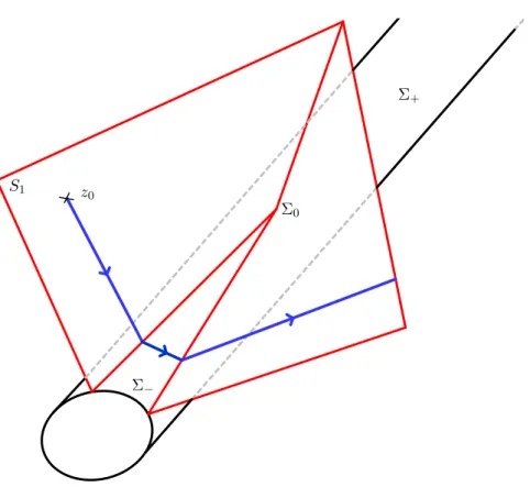
Lemma 2. There exists a codimension one submanifold S1 “ŤzPNWspzq—the set of
initial conditions leading to Σ—preserved by the flow, and on which it is locally smooth. More precisely, the map z : r0, tfs ˆ S1z∆ Ñ O¯z is smooth,
S1
´
`
0
z0
Figure 1 - Stratification of the flow into regular submanifolds
The system (7) is autonomous, so there is a unique extremal passing through ¯z, besides, this is happening in finite time t. Indeed, notice that z fiÑ cos ◊H01pzq ` sin ◊H02pzq “
´ar2pzq ´ H122pzq is smooth, and as such, bounded on O¯z. It is also negative, and
note C † 0 a negative upper bound. Now by considering the dynamics of fl, see that 9flpsq § flpsqC. Hence, by Gronwall’s lemma flpsq † flp0qeCs. Now the time interval before
reaching satisfies:
t† ª8
0 flpsqds † flp0q{C † 8.
From now on we will investigate the flow regularity, starting by:
Lemma 2. There exists a codimension one submanifold S1“ \zPNWspzq - namely, the
set of initial conditions leading to - preserved by the flow, and on which it is locally smooth. More precisly, the map z : r0, tfs ˆ S1z Ñ O¯z is smooth,
where “ tp¯tpz0q, z0q, z0P S1u, ¯tpz0q being the switching time of the extremal passing
through z0.
Proof of Lemma 2. We begin the proof by showing that S1 is a well defined
codi-mension 1 submanifold. Recall that the Jacobian of the vector field has a convenient 9
Figure 1: Stratification of the flow into regular submanifolds.
where ∆ “ tp¯tpz0q, z0q, z0 P S1u, ¯tpz0q being the switching time of the extremal passing
through z0.
Proof of Lemma 2. We begin the proof by showing that S1 is a well defined
codi-mension 1 submanifold. Recall that the Jacobian of the vector field has a convenient spectrum on N: A 6-dimensional kernel,
cos θ´H01` sin θ´H02“ ´
b
r2´ H122 ,
and `ar2´ H122 . As such, the flow is normally hyperbolic to N, then V “ŤzPNWspzq
is the so-called stable manifold of N. V is smooth by theorem 3 since there is no dilata-tion nor contracdilata-tion on T N. Then the submanifold we are looking for is S1 “ V Xtρ ą 0u,
and dim S1 “ dim N ` dim Wspzq “ 7. It remains to show that the map z : pt, z0q P
r0, tfs ˆ S1z∆ ÞÑ zpt, z0q P O¯z is smooth. Let’s set ¯tpz0q “
ş8
0 ρps, z0qds the contact time
with the singularity Σ, we know that ¯tpz0q ă 8. The flow is smooth in the time s, hence
z0 ÞÑ ρps, z0q is smooth and by the classical dominated convergence argument, ¯tpz0q is
smoothly depending on z0 P O¯z. Obviously z : pt, z0q P r0, ¯tpz0qq ˆ S1 ÞÑ zpt, z0q P O¯z is
contact point with the singular locus Σ is depending smoothly on the initial condition on S1, more precisely, the map z0 P S1 ÞÑ zp¯tpz0q, z0q is smooth. It is straightforward
by writing zp¯tpz0q, z0q “ ş80 Xpzps, z0qqds ` z0. The integrand is bounded uniformly
with respect to z0, indeed, s ÞÑ zps, z0q is only parameterizing the stable manifold
Wspzp¯tpz0q, z0qq Ă O¯z, but this neighborhood is relatively compact (and independent of
z0), and the vector field X is bounded on O¯z. Thus this integral is smooth with respect
to the parameter z0. Now notice that pt, z0q ÞÑ zpt ´ ¯tpz0q, zp¯tpz0q, z0qq “ zpt, z0q is an
extremal initializing on Σ at time ¯tpz0q. By the symmetry t ÞÑ ´t, this situation is
analogous to the previous one, this map is smooth as long as t ‰ ¯tpz0q, which conclude
the proof of Lemma 2. l
We now know that the flow is smooth outside of S1 and restricted to S1, we also know
that it is Lipschitz with respect to the time t. It remains to prove its global continuity on O¯z.Let z0, z1 P O¯z, t, t1 in r0, tfs and Oδ Ă O¯zbe a small neighborhood of ¯z. Thanks
to the previous assumption, we can assume without loss of generality, that z0 P S1,
z1 P O¯zzS1 and that the extremal from z0 is passing throw ¯z. We would like to control
de quantity |zpt, z0q ´ zpt1, z1q|. Let ε ą 0, and note t0, the contact time with Oδ, and
t10 the exit time from this neighborhood: Namely t0 “ inftt P R, s. t. zpt, z0q P Oδu.
If z0 and z1 are close enough, |zpt0, z0q ´ zpt0, z1q| ă ε{2; simply because the flow is
continuous when the singular locus is not crossed yet. We will use the following Lemma to conclude:
Lemma 3 ([2]). For all δ ą 0 there exists a neighborhood Oδof ¯z in which every extremal
spends a time interval uniformly (that is not depending on the extremal) smaller than δ.
Proof of Lemma 3. We will prove it in a neighborhood O¯z´ of ¯z´, the situation
being symmetric around ¯z`, and an extremal in Σ spending 0 time t. Let’s define
Oδ “ tz P O¯z´, ρă δ, |θ ´ θ´| ă δu, z ÞÑ cospθqH01pzq ` sinpθqH02pzq is smooth and thus
bounded on Oδ. Now set
Mδ“ sup zPOδ
cospθqH01pzq ` sinpθqH02pzq,
remember it is negative on O¯z´. Then, for any extremal in Oδ, ρρ9psqpsq ď Mδ, which implies
ρpsq ă ρp0qeMδs.
So that, we can control its time interval in 0δ by
∆Oδtă ż8 0 ρp0qe Mδsds“ ´ R Mδ ,
this quantity tends to 0 when R does, and the lemma is proved. Then, with a good choice of Oδ, |zpt10, z0q´zpt0, z0q| ď ε{2, and |zpt10, z0q´zpt0, z1q| ď |zpt10, z0q´zpt0, z0q|`
|zpt0, z0q ´ zpt0, z1q| ď ε. Now notice that, zpt, z0q “ zpt ´ t10, zpt10, z0qq, and we use the
Remark 1. In the case ¯z P Σ´, ie, the only case when switching occur, we can quantify
the jump on the control at a switching time ¯t in terms of Poisson brackets:
up¯t˘q “ pcos θ˘,sin θ˘q “ 1 r2p´H02H12˘ H01 b r2´ H122 , H01H12˘ H02 b r2´ H122 q.
Case ¯z P Σ`. The dynamics in the initial time is still given by:
$ ’ ’ ’ ’ ’ ’ & ’ ’ ’ ’ ’ ’ % 9x“ F0pxq ` cospθqF1pxq ` sinpθqF2pxq 9ρ“ cos θH01` sin θH02 9θ “ 1 ρpH12` cospθqH02´ sinpθqH01q 9H01“ H001` cos θH101` sin θH201 9H02“ H002` cos θH102` sin θH202. (11)
In particular, by lemma 1 we already know 9θ is everywhere nonzero. Without loss of generality let’s assume ρ 9θ “ H12` cospθqH02´ sinpθqH01 ą 0 on O¯z. The following
lemma implies the results on this case:
Lemma 4. In a neighborhood O¯z of ¯z P Σ` we have the estimate: DK, c ą 0, @t s.t
zptq P O¯z, ρptq ě Kρ0e´ct.
Proof of the Lemma. Without loss of generality let’s assume H12 ` cospθqH02´
sinpθqH01 ą 0 on O¯z. O¯z is relatively compact, and as such, the continuous map u :
z Ñ H12pzq ` cospθpzqqH02pzq ´ sinpθpzqqH01pzq, is bounded from below and above by
two positive constant c1 and c2: c2 ą upzq ą c1 ą 0 for all z P O¯z. One can notice
that d
dtpρpH12` cos θH02´ sin θH01qq “ ρp 9H12 ` cos θ 9H02´ sin θ 9H01q. By remark 9,
9Hij “ H0ij` cos θH1ij` sin θH2ij which also define a smooth map. As such ρp 9H12`
cos θ 9H02´ sin θ 9H01q ě a with a ă 0 some constant. Then we have:
d
dtpρuq ě aρ ô ρptquptq ě ρ0up0q ` a
żt
0 ρpsqds.
Now using Gronwall’s lemma: ρptquptq ě ρ0up0qeA şt
01{upsqds.Finally
ρptq ě ρ0c1
c2e
a{c2t.
We conclude the proof of theorem 2 by taking c “ ´a{c2 ą 0 and K “ c1{c2. For
extremals lying in Σ`, the following proposition holds:
Proposition 2. There exists a singular flow inside Σ` and Σ0, on which we have the
control feedback: u “ 1
H12p´H02, H01q, and the singular flow is smooth. It is solution of
the Hamiltonian system H “ H0´HH0212H1`
H01
Proof. H1 and H2 are identically vanishing along a singular extremal, and so are they
derivative with respect to the time t. Then, for the time interval on which dHi
dt pzptqq “
H0ipzptqq ` ujHjipzptqq “ 0 for i “ 1, 2. Those identities give the wanted feedback.
Since |u| ď 1, this cannot happen in Σ`. So H12 cannot be zero, and the singular flow
is smooth. l
Remark 2. It has been noticed in [8] that extremals lying in Σ` cannot be optimal by the Goh condition.
3
Regular-singular transition
In the applications, whenever the distribution is involutive the interesting case is Σ´,
and we have the stratification defined in the previous section. This stratification of the flow raises the question of the transition: How does the flow behave when one is getting close to the stratum S1? We answer that question by considering the Poincaré map
between two well chosen sections. Recall the dynamic in the time s: $ ’ ’ ’ ’ ’ ’ & ’ ’ ’ ’ ’ ’ % x1 “ ρpF0pxq ` cospθqF1pxq ` sinpθqF2pxqq ρ1 “ ρpcos θH01` sin θH02q θ1“ H12` cospθqH02´ sinpθqH01 H011 “ ρpH001` cos θH101` sin θH201q H021 “ ρpH002` cos θH102` sin θH202q.
in polar coordinates on the Poisson brackets: pH01, H02q “ rpcos φ, sin φq one gets:
$ ’ & ’ % ρ1 “ rρ cospθ ´ φq θ1 “ H12´ r sinpθ ´ φq ξ1“ ρhpρ, θ, ξq (12)
where ξ “ px, r, φq and h is a smooth function. We can set ψ “ θ ´ φ, rescale the time according to dv “ rds, and study a system with the following structure (the derivation still being noted1):
$ ’ & ’ % ρ1 “ ρ cos ψ ψ1 “ gpρ, ψ, ξq ´ sin ψ “ Gpρ, ψ, ξq ξ1 “ ρhpρ, ψ, ξq (13)
where g, h are smooth functions defined on an open set O of RˆRˆD, D being a compact domain of Rk; h has values in Rkand gpρ, ψ, ξq “ apξq`ρbpξ, ψq`Opρ2q and |g| ă 1 on O.
(This comes from the fact that H12 is a smooth function in pρ cos θ, ρ sin θq.) Equilibria
occur when ρ “ 0, G “ 0 and are semi-hyperbolic, since they’re outside tψ “ ˘π{2u. More precisely, it was shown in the last section that the flow of this system is normally hyperbolic to the manifold tρ “ 0u X tG “ 0u. For each ξ, there are two equilibria z˘.
Thanks to the structure of g, we get Bg
Bψp0, ψ, ξq “ 0, thus BGBψp0, ψ, ξq “ ´ cos ψ ‰ 0.
function theorem. Equilibria are then given by p0, ψ12pξq, ξq coordinates, and define two
codimension two submanifolds. In each equilibria, the stable and unstable manifolds are of dimension one. Their reunion form a codimension one submanifold, S12“ŤξWspz12q.
S1 is thus the submanifold of initial condition leading to an equilibrium (in infinite
time). The aim of the following work is to study the regular-singular transition, or more precisely, the type of singularity occurring when one crosses S1.
Introducing ω “ ψ´ψpξq along tG “ 0u (the analysis is similar for ψ2on the unstable
manifold), we will study p13q near ω „ 0. The change of coordinates pρ, ψ, ξq ÞÑ pρ, ω, ξq
gives $ ’ & ’ % ρ1 “ ρ cospω ` ψpξqq ω1 “ gpρ, ω ` ψpξq, ξq ´ sinpω ` ψpξqq ´ ρBψBξpξq.hpρ, ω ` ψpξq, ξq ξ1 “ ρhpρ, s ` ψpξq, ξq
As g has the form given by piiq, gpρ, ω ` ψpξq, ξq “ apξq ` ρbpω ` ψpξq, ξq ` Opρ2q, and
gp0, ψpξq, ξq “ sinpψpξqq “ apξq. So that system p1q is equivalent to
$ ’ & ’ % ρ1 “ λpξqρp1 ` Opω2qq ω1 “ βpξqρ ´ λpξqω ` Oppρ ` |ω|q2q ξ1“ ρpγpξq ` Opρ ` |ω|qq (14)
with λpξq “ cospψpξqq and β, γ smooth functions (depending on the derivatives of g, h). The Jacobian matrix of (14) is
¨ ˝ λpξq 0 0 βpξq ´λpξq 0 γpξq 0 0 ˛ ‚.
Let us now find a change of coordinates making this Jacobian diagonal: pρ, ω, ξq ÞÑ pρ, ˜ω, ˜ξq “ pρ, ω ` Apξqρq, ξ ` Bpξqρq. We get ˜ω1 “ ω1`BA
Bξpξq.ξ1ρ` Apξqρ1 “
ω1 ` Apξqρ ` Opρ2q. Thus ˜ω1 “ pβpξq ` 2Apξqλpξqqρ ´ λpξq˜ω ` Oppρ ` |ω|q2q and by
picking A “ ´β
λ we obtain what we were looking for: Indeed, with this change of
vari-ables, Oppρ ` |ω|qkq “ Opp˜ρ ` |˜ω|qkq for all k. Now, ˜ξ1 “ ξ1 ` BA
Bξpξq.ξ1ρ` Bpξqρ1 “
ρpγpξq ` Bpξqλpξqq ` Oppρ ` |ω|q2q and we pick Bpξq “ ´γλ. Slightly abusing of the
notations (except for ρ), we still note the new variables pρ, ω, ξq and obtain the new
vector field $ ’ & ’ % ρ1 “ λpξqρp1 ` Opρqq ω1“ ´λpξqω ` Oppρ ` |ω|q2q ξ1 “ ρOpρ ` |ω|q (15)
System (15) is smoothly equivalent to
Y : $ ’ & ’ % ρ1 “ ´ρp1 ` Opρqq ω1 “ ω ` Oppρ ` |ω|q2q ξ1 “ ρOpρ ` |ω|q (16)
field $ ’ & ’ % fl1“ ⁄p›qflp1 ` Opflqq s1“ ´⁄p›qs ` Oppfl ` |s|q2q ›1“ flOpfl ` |s|q (14) System (14) is smoothly equivalent to
Y : $ ’ & ’ % fl1“ ´flp1 ` Opflqq s1“ s ` Oppfl ` |s|q2q ›1“ flOpfl ` sq (15) The Jacobian of this system is diagonal and even constant. Let us now state a smooth normal form theorem:
Proposition 3 (C8-normal form). Let u “ fls, then there exist A, B, C smooth
func-tions on a neighborhood of D ˆ 0u such that Y is equivalent to
Y8: $ ’ & ’ % fl1“ ´flp1 ` uApu, ›qq s1“ sp1 ` uBpu, ›qq ›1“ uCpu, ›q (16) Under this change of coordinates, the globally invariant manifold S´, fibered by stable
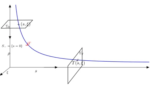
manifolds, becomes ts “ 0u, and the equilibria are tp0, 0, ›qu. We can now make a precise statement: For given fl0 et sf, both positive, consider the two sections 0 Ä tfl “ fl0u
and f Ä ts “ sfu. As 0 is transverse to ts “ 0u, it can be parameterized by ps, ›q
coordinates. Similarly, f is transverse to tfl “ 0u and can be parameterized by pfl, ›q
coordinates. s fl ps, ›q Tps, ›q S´“ ts “ 0u 0 f › T Fig-ure 2 - Poincaré map between the two sections
14
Figure 2: Poincaré map between the two sections.
The Jacobian of this system is diagonal and even constant. Let us now state a smooth normal form theorem:
Proposition 3 (C8-normal form). Let u “ ρω, then there exist A, B, C smooth
func-tions on a neighborhood of D ˆ 0u such that Y is equivalent to
Y8: $ ’ & ’ % ρ1“ ´ρp1 ` uApu, ξqq ω1 “ ωp1 ` uBpu, ξqq ξ1 “ uCpu, ξq (17)
Under this change of coordinates, the globally invariant manifold S´, fibered by stable manifolds, becomes tω “ 0u, and the equilibria are tp0, 0, ξqu. We can now make a precise statement: For given ρ0 et ωf, both positive, consider the two sections Π0 Ă tρ “ ρ0u
and Πf Ă tω “ ωfu. As Π0 is transverse to tω “ 0u, it can be parameterized by pω, ξq
coordinates. Similarly, Πf is transverse to tρ “ 0u and can be parameterized by pρ, ξq
coordinates.
Theorem 4. Let T : Π0 Ñ Πf be the Poincaré mapping between the two sections,
Tpω0, ξ0q “ pρpω0, ξ0q, ξpω0, ξ0qq. Then, T is a smooth function in pω0ln ω0, ω0, ξ0q as
there exist smooth functions R and X defined on a neighborhood of t0u ˆ t0u ˆ D such that
Tpω0, ξ0q “ pRpω0ln ω0, ω0, ξ0q, Xpω0ln ω0, ω0, ξ0qq.
Thus, T belongs to the log-exp category.
for the minimum time Kepler problem. Recall we had x3pt, z0q “ a a2` c2p a pat ` bq2` pct ` dq2´ab2` d2q ´cpaad2` c´ bc2q3{2 „ argshˆpa2` c2qt ` ab ` cd ad´ bc ˙ ´ argsh ˆ ab` cd ad´ bc ˙ ` x3p0q (18)
giving the regularity. When one crosses Σ the determinant ad ´ bc becomes 0, and one indeed get singularities of the form ”z ln z”.
Proof of Theorem 4. Before proving the normal form result, let’s demonstrate how it implies Theorem 4. First, note that system (17) is equivalent to
$ ’ & ’ % ω1 “ ω ρ1“ ´ρp1 ` uApu, ξqq ξ1 “ uCpu, ξq (19)
with A standing now for A´B
1`uB, and C for 1`uBC . It has the same trajectories, and thus
the same Poincaré mapping between the two sections. The transition time is given by the first equation: tpω0q “ lnpωf{ω0q. (The singular-regular transition occurs when ω0Ñ 0,
and the transition time tends to infinity.) Still noting u “ ρω, (19) implies #
u1 “ ´u2Apu, ξq,
ξ1“ uCpu, ξq, (20)
that we want to integrate from an initial condition on Π0 in time tpω0q. We extend
this system by the trivial equation ω1
0 “ 0, and denote ϕ its associated flow. Then,
Tpω0, ξ0q “ ϕplnpωf{ω0q, ω0, ρ0ω0, ξ0q (on Π0, u0 “ ρ0ω0). It is not the form we are
looking for since lnpω{ω0q is not regular at ω0 “ 0, but we have the following estimate
on the u coordinate of the flow.
Lemma 5. There exists a constant M such that, for small enough ω0 ą 0, ξ P D, and
integration time t ď lnpωf{ω0q,
0 ď upt, ω0, ρ0ω0, ξ0q ď Mω0.
Proof of the Lemma. Compare the dynamics of u in (20) with v1 “ ´v2, which
integrates according to vpt, v0q “ 1 ` vv0 0t for v0 ą 0. So vplnpωf{ω0q, ρ0ω0q “ ρ0ω0 1 ` ρ0ω0lnpωf{ω0q ,
Let us now make a change of time and consider the following rescaled system: $ ’ & ’ % s10“ 0, u1“ ´pu2{ω0qApu, ξq, ξ1 “ pu{ω0qCpu, ξq. (21)
For ω0 ą 0, its flow ˜ϕis well defined and the Poincaré mapping is obtained by evaluating
it in time ω0lnpωf{ω0q,
Tpω0, ξ0q “ ˜ϕpω0lnpωf{ω0q, ω0, ρ0ω0, ξ0q.
We use the blow up on tu “ ω “ 0u to prove that T has the required form. Set
fpu, ω, ξq “ pη, ω, ξq with η “ u{ω: In coordinates pω, η, ξq, the pulled back system
writes Z : $ ’ & ’ % ω01 “ 0, η1“ ´η2Apηω0, ξq, ξ1 “ η Cpηω0, ξq, . (22)
The vector field Z is actually smooth. The blow up map f send a cone ´η0ω ď u ď η0s
on a rectangle ´η0 ď η ď η0, ´ω0 ď ω ď ω0. According to the previous Lemma, we
only need to evaluate its flow ˆϕpt, ω0, η0, ξ0q on a band ω0 P r´ω1, ω1s, η0 P r´M, Ms,
ξ P D, to compute ˜ϕis time ω0lnpωf{s0q. As ˆϕ“ pˆη, ˆξq is smooth on such a band, we
eventually get
Tpω0, ξ0q “ pˆηpω0lnpωf{ω0q, ω0, ρ0, ξ0q, ˆξpω0lnpωf{ω0q, ω0, ρ0, ξ0q,
which has the desired regularity. Box
Remark 3. Notice that when ω Ñ 0, the Poincaré map goes in the invariant submanifold
tρ “ 0u, although in infinite time. Let us finally prove Proposition 3.
Proof of Proposition 3. Let us first state a generalization of the Poincaré-Dulac theorem. First we introduce some notation. Note Hl the space of homogeneous
poly-nomials of degree l in Rn with smooth coefficients in ξ P Rk. We recall that for a linear
vector field X which does not depends on ξ (and has no component in the ξ direc-tion), Hl “ ImrX, .s
|Hl` kerrX, .s|Hl. A vector field Z is said to be resonant with X if
Z P kerrX, .s.
Lemma 6. Let Xpx, ξq be a smooth vector field in Rnˆ Rk, Xp0, ξq “ 0. Note X1 its
linear part. Then, if X1 does not depend on ξ, there exist giP HiXkerrX1, .s, i “ 2, . . . , l
and a smooth vector field Rl with zero l-jet such that X is smoothly conjugate to in a
neighborhood of zero to:
Proof of Lemma 6. We will follow [18] and reason by induction on l, then treat the case l “ 8. For l “ 1, the result is trivial: X “ X1 ` R1 where R1 has zero first
jet in zero. Suppose now that g1, . . . , gl´1, and Rl´1 are as in lemma 6, l ě 2. Rl´1
has a zero l ´ 1 jet (in zero), and then can be written as Rl´1 “ rX1, Zs ` gl ` Rl,
where Z P Hl, g
l P kerrX1, .s and Rl is a smooth vector field with zero l-jet. rX, Zs “
rX1, Zs `řli“2rgi, Zs ` rRl´1, Zs “ rX1, Zs ` R1l, where R1l has zero l-jet. Now, note
φZ the flow of Z, and consider pφtZq˚X :“ Xt. We have dtdXt“ rX, Zs “ rX1, Zs ` R1l,
so that Xt “ X0 ` trX
1, Zs ` Rl,t, with jlpRl,tqp0q “ 0. Since Z is a homogeneous
polynomial of degree l, it has zero l ´ 1 jet, and X and Xt have the same l ´ 1 jet,
that means X0 “ X
1` g2` ¨ ¨ ¨ ` gl` rX1, Zs. Finally, we chose t “ ´1 to get X´1 “
X1` g2` ¨ ¨ ¨ ` gl` Rl,´1, and φ´1Z conjugates the two vector field, which ends the proof
of the finite case. The above construction provide a sequence of formal diffeomorphisms
ϕl“ φ´1Z (Z P Hl) with pϕlq˚X “ X1` g2` ¨ ¨ ¨ ` gl` Rl. Also notice that ϕl and ϕl`1
have the same l-jet. This define a sequence of coefficient glpξq for all l. l Now remark
that a generalization of Borel theorem, proved by Malgrange in [13] show that there exists a smooth function ψ such that the l jet of ϕl and ψ are identical for all l P N.
We can also realize, using the same theorem, the formal series given by the resonant monomials by a smooth vector field X8. Thus we have ψ
˚pXq “ X8` R8, where R8
has zero infinite jet. Thus, we begin by looking for monomials that are resonant with the linearized vector field of Y , Y1 “ ´ρBρB ` sBωB (monomials X for whom rY1, Xs “ 0).
First notice that the Lie bracket with Y1 treat ξ as a constant: The map X ÞÑ rY1, Xs
is linear in ξ. Such monomials can be written apξqρiωj B
Bρ, bpξqρiωjBωB , and cpξqρiωjBξB. We get: rY1, apξqρisj B Bρs “ pi ´ j ´ 1qapξqρiωjBρB rY1, bpξqρiωj B Bωs “ pi ` 1 ´ jqbpξqρiωj B Bω and rY1, cpξqρiωj B Bξs “ pi ´ jqcpξqρiωj B Bξ. The monomials we are looking for are thus: apξqρuk B
Bρ, bpξqsukBωB and cpξqukBξB, k P N.
The lemma allow us to state that the infinite jet of Y can be formally developed on the resonant monomials, ie, Y is formally conjugate to
W : $ ’ & ’ % ρ1 “ ´ρp1 `řiě1aipξquiq ω1 “ ωp1 `řiě1bipξquiq ξ1“ ρřiě1cipξqui .
It remains to realize those series by smooth functions. By the remark above, there exist Y8 a smooth vector field on O such that W “ Y8` R8 where R8 is a smooth
function with zero infinite jet along D. At this stage we have Y is smoothly equivalent to Y8` R8.
The last step consists in killing the flat perturbation R8. This can be achieved
Y1 :“ Y8` R8, we search for a one parameter family (path) of diffeomorphism (gt)
such that
gt˚Y0 “ Yt, (23)
Yt being a path of vector fields joining Y0 and Y1. Consider the linear path Yt “
p1 ´ tqY0` tY1, t P r0, 1s. Differentiating (23) with respect to t we get
B
Btpg˚tY0q “ 9Yt“ Y1´ Y0“ R8. (24)
Now, the family gtdefine a family of vector fields Ztby Ztpgtpxqq “ BtBgtpxq|t, reciprocally
by integrating Zt we obtain the desired path of diffeomorphism. Thus (24) can be
rewritten
rYt, Zts “ R8. (25)
We just showed that getting rid of the flat perturbation R8 boils down to find a solution to the equation (25). It has been proved in [17], theorem 10, that this equation has a
solution. l
4
Application to mechanical systems
In this section, we specify our study to mechanical systems coming from a potential, and go further in the particular case of orbit transfer problem with gravitational coplanar two or three body potential. Consider a system of the form :q ` ∇V pqq “ 0. Let
q P M “ R2zt´µ, 1 ´ µu be the position vector, and note µ the mass ratio of the
two primaries. The dynamics of the controlled restricted elliptic three-body problem (CETBP) is the following - q1 and q2 are the positions of the two primaries, which by
definition, are in elliptic motion around their center of mass: :q` ∇Vµpt, qq “ u,
with Vµpt, qq “ |q´q1´µ1ptq| `|q´qµ2ptq|.One can notice that when µ “ 0, we are in the
Kep-lerian case. The non-autonomous Maximized Hamiltonian given by a non-autonomous version of the Maximum Principle is
Hpt, zq “ pq.v´ ∇Vµpt, qq.pv` |pv|, with z “ px, pq.
with of course pq, (resp. pv) being the adjoint coordinate of q, (resp. v).
The controlled circular restricted three body problem (CRTBP) is a reduction of the (CETBP) where the two primaries are in circular motion around their center of mass. Its dynamics can be express as an autonomous system, in the rotating frame. Written on the convenient affine control system form: x “ pq, vq,
9x“ F0pxq ` u1F1pxq ` u2F2pxq with F0pxq “ F0pxq “ v.Bq` p´q ` p1 ´ µq q` µ |q ` µ|3 ` µ q´ 1 ` µ |q ´ 1 ` µ|3 ` 2Jvq.Bv,
F1pxq “ Bv1, F2pxq “ Bv2 in Cartesian coordinates. The maximized Hamiltonian of the
(CRTBP) given by the maximum principle is:
Hpzq “ pq.v´ Jµpq, uq.pv` |pv|, with Jµpq, vq “ ´q ` p1 ´ µq q` µ |q ` µ|3 ` µ q´ 1 ` µ |q ´ 1 ` µ|3 ` 2Jv.
Before applying the result of section 2, let us make the following important remark: In both cases, the distribution generated by F1 and F2 is involutive as the two vector fields
actually commute:
rF1, F2s “ 0. (26)
Proposition 4. Assumption (A) is check for the Keplerian and circular restricted
three-body problem.
This is actually the consequence of a more general statement (see [8] for the proof). Lemma 7. A second order controlled system on Rn
:q` gpq, 9qq “ u
is a control-affine system on R2mwith an involutive distribution tF
1, . . . , Fmu and a drift
F0 such that tF1, . . . , Fm, F01, . . . , F0mu has maximum rank.
Local properties. The following proposition has been proved in [9] is a direct conse-quence of remark 1, and of (26).
Proposition 5. The switching correspond to instant rotation of angle π of the control
(π-singularity). If t is a switching time, upt´q “ ´upt`q.
Now applying theorem 2, we obtain:
Proposition 6. Let O¯z be a neighborhood of ¯z P Σ: The local extremal flow of the
minimum-time restricted circular three-body problem is piecewise smooth, and stratified into: O¯z “ S0 Y S1Y Σ, S1 being the co-dimension one manifold of initial conditions
leading to the singularity, and S0 its complementary. The flow is smooth on each strata
and continuous on O¯z:
- if z0 P S1 the extremal from z0 has exactly one π-singularity in O¯z,
- Otherwise the extremal from z0 has no π-singularity.
Besides, the regular-singular transition is Lipschitz continuous.
Proof. Since (A) is checked, we just need to insure that Σ “ Σ´ in this case. However
H12” 0 because of (26), implying H012 pzq ` H022 pzq ą H12pzq2 for all z P T˚M. The last
Global properties. Those switchings are the so-called π-singularities. Since there is no accumulation of switching points, there is only a finite number of such singularities on a time interval r0, tfs. We are now going to investigate global properties of such
switching. Namely, the next proposition bounds the number of π-singularity along a time optimal trajectory.
Definition 2. We define δ “ infr0,tfs|qptq|, δ1“ infr0,tfs|qptq ´ q
1ptq|, δ2“ inf
r0,tfs|qptq ´
q2ptq|. This quantities represents the distance to the collisions in the two body, and
restricted three-body problems respectively. Finally note δ12pµq “ pp1´µqδδ13δ2 2`µδ31q1{3.
Estimate on the global number of switching can be obtain by Sturm like theorems, we denote by rxs the integer part of a real number x:
Proposition 7. - In the Keplerian case, there is at least a time interval of length πδ3{2
between two π-singularities. On a time interval r0, tfs the maximum amount of such
singularities is N “ r tf
πδ3{2s.
- In the controlled restricted three-body problem with a mass ratio µ, there is at least a time interval of length πδ12pµq3{2 between two π-singularities. On a time interval r0, tfs
the maximum amount of such singularities is N “ r tf
πδ12pµq3{2s.
One can notice that δ12p0q “ δ, which makes the proposition coherent. The proof is a
immediate consequence of the more general lemma:
Lemma 8. Let us consider the minimum-time control system coming from a C2potential
V : R ˆ O Ñ R, O Ă Rn,
:q` ∇Vtpqq “ u, }u} ď 1. (27)
Let Atpqq P SnpRq a continuous matrix, such that for all time t, and q P O, Atpqq ě
∇2Vtpqq, then the following statement holds: If ¯t1 and ¯t2 are switching times for (27),
there exists a non trivial solution of :y ` Atpqptqqy “ 0 vanishing in ¯t1 and t1 ă ¯t2.
Proof of Lemma 8. Applying the P.M.P. to p27q, one gets the maximized Hamiltonian
H˚pq, v, pq, pvq “ pq.v´pv.∇Vtpqq`|pv|, and the feedback u˚ “ |ppvv|. It remains to study
the zeros of the adjoint state pv to have access to the switching times. The equation on
pv is a second order linear equation:
:pv` ∇2qVtpqqpv“ 0. (28)
The following Sturm-like theorem is due to Morse and will allow us to conclude (see [14]):
Theorem 5 (Morse). Let a, b P R, with b ą a. Consider the two linear second order
equations
z2` P ptqz “ 0, (29)
and
z2` Qptqz “ 0, (30)
with P ptq, Qptq be two symmetric continuous n ˆ n matrices, such that Qptq ´ Pptq ě 0, and assume there exists a ¯t with Qp¯tq ´ Pp¯tq ą 0. If (29) has a non trivial solution y, ypaq “ ypbq “ 0, then (30) has a non trivial solution which vanishes in a and c ă b.
If Atpqq is a matrix as mentioned in Lemma 8, Morse’s theorem gives the result by taking
Qptq “ Atpqptqq and the lemma is proved.
Proof of Proposition 7. We will only be interested the second statement, since it implies the first one. Recall the dynamics of the third mass is:
:q “ ´∇qVµpt, qq ` u,
with Vµpt, qq “ ´|q´q1´µ1ptq| ´|q´qµ2ptq|, the non-autonomous potential. Let
Atpqq “ ˜ 1 `|q´q1´µ1ptq|3 `|q´qµ2ptq|3 0 0 |q´q1´µ1ptq|3 `|q´qµ2ptq|3 ¸ P M2pRq.
A straightforward calculation shows that
detpAtpqq ´ ∇2qVµpt, qqq “ 3
„
p1 ´ µqpq|q ´ q2´ q121|q52 ` µpq|q ´ q2´ q222|q52
ą 0
as long as we don’t have q2ptq “ q12ptq “ q22ptq. But this cannot happen on the whole
trajectory, and so Morse’s theorem apply. By our lemma above, the minimum-time interval between two switching times is greater than the time interval between conjugate times of the solutions of: z2
2 ` p|q´q1´µ1ptq|3 ` |q´qµ2ptq|3qz2 “ 0. But of course, |q´q1´µ1ptq|3 `
µ
|q´q2ptq|3 ď 1´µδ3
1 `
µ
δ32, and by Sturm’s theorem in dimension one, solutions of this equation
cannot have two conjugate times in a interval of length smaller than c π
1´µ δ31 `
µ δ32
. Finally, the distance between two switching times is in fact greater than
πδ13{2δ3{22
a
p1 ´ µqδ23` µδ13 “ πδ12pµq 3{2.
l One of the natural extensions for this work is to study the influence of averaging on the stratification. Indeed, in the controlled Kepler problem, one can average with respect to the fast angle, [8, 5] and reduce the dimension of the problem. Thus, the projection of the singular locus Σ becomes of codimension one and extremals will cross it generically. Fortunately, averaging regularizes the Hamiltonian and the study of the singularities still occurring has been initiated in the previously cited papers and should be pursued.
Acknowledgements. The authors thank Jean-Pierre Marco for many and fruitful exchanges on the work presented in this paper.
References
[1] Agrachev, A. A.; Biolo, C. Optimality of broken extremals. arXiv:1709.07775, 2017. [2] Agrachev, A. A.; Biolo, C. Switching in time-optimal problem: The 3D case with
2D control. J. Dyn. Control Syst., 23 (2017), no. 3, 577–595.
[3] Agrachev, A. A.; Sachkov, Y. L. Control theory from the geometric viewpoint. Springer, 2004.
[4] Biolo, C. Switching in time-optimal problem. PhD thesis, SISSA, 2017.
[5] Bombrun, A. Pomet, J.-B. The averaged control system of fast oscillating control
systems. SIAM J. Control Optim. 51 2016, 2280–2305.
[6] Bonnard, B.; Henninger, H. C.; Nemcová, J.; Pomet, J.-B. Time versus energy in the averaged optimal coplanar kepler transfer towards circular orbits. Acta Appl.
Math. 135 (2015), no. 1, 47–80.
[7] Caillau, J.-B., Combot, T., Féjoz, J., Orieux, M. Non-integrability of the minimum time Kepler problem. Submitted to J. Geom. Phys. (2018)
[8] Caillau, J.-B.; Daoud, B. Minimum time control of the restricted three-body prob-lem. SIAM J. Control Optim. 50 (2012), no. 6, 3178–3202.
[9] Caillau, J.-B.; Noailles, J. Coplanar control of a satellite around the Earth. ESAIM
Control Optim. and Calc. Var. 6 (2001), 239–258.
[10] Chen, Z.; Caillau, J.-B.; Chitour, Y. L1-minimization for mechanical systems. SIAM
J. Control Optim. 54 (2016), no. 3, 1245–1265.
[11] L. van den Dries; Macintyre, A.; Marker, D. The elementary theory of restricted analytic fields with exponentiation, Ann. of Math., 140, (1994), no. 1, 183–205, [12] Hirsch, M. W.; Pugh, C. C.; Shub, M. Invariant manifolds. Springer, 2006. [13] Malgrange, B. Ideals of differentiable functions. Oxford University Press, 1967. [14] Morse, M. A generalization of the sturm separation and comparison theorems in
n-space. Math. Ann. 103 (1930), no. 1, 52–69.
[15] Pesin, Y. B. Lectures on partial hyperbolicity and stable ergodicity. European Math-ematical Society, 2004.
[16] Poincaré, H. Les méthodes nouvelles de la mécanique céleste. Gauthier-Villars, 1892. [17] Roussarie, R. H. Modèles locaux de champs et de formes. Société Mathématique de
France, 1976.